Viscoelasticity and shear flow of concentrated, non-crystallizing colloidal suspensions:
Comparison with Mode-Coupling Theory

Abstract

We present a comprehensive rheological study of a suspension of thermosensitive particles dispersed in water. The volume fraction of these particles can be adjusted by the temperature of the system in a continuous fashion. Due to the finite polydispersity of the particles (standard deviation: 17%), crystallization is suppressed and no fluid-crystal transition intervenes. Hence, the moduli $G^{\prime}$ and $G^{\prime\prime}$ in the linear viscoelastic regime as well as the flow curves (shear stress $\sigma(\dot{\gamma})$ as the function of the shear rate $\dot{\gamma}$) could be measured in the fluid region up to the vicinity of the glass transition. Moreover, flow curves could be obtained over a range of shear rates of 8 orders of magnitude while $G^{\prime}$ and $G^{\prime\prime}$ could be measured spanning over 9 orders of magnitude. Special emphasis has been laid on precise measurements down to the smallest shear rates/frequencies. It is demonstrated that mode-coupling theory generalized in the integration through transients framework provides a full description of the flow curves as well as the viscoelastic behavior of concentrated suspensions with a single set of well-defined parameters.

1 Introduction

The flow behavior of concentrated suspensions of hard sphere particles in a shear flow is a long-standing problem in colloid physics [Russel et al. (1989), Larson (1999)]. The most prominent feature of these systems is the strong increase of the zero-shear viscosity with increasing volume fraction $\phi$. Concomitantly, there is a strong increase of the storage modulus $G^{\prime}$. Moreover, with increasing shear rate a marked shear thinning sets in where the relative viscosity $\eta/\eta_{S}$ ($\eta_{S}$: viscosity of solvent) is lowered considerably. These general features are also observed for solutions of soft colloidal particles as e.g. a solution of star polymers in a suitable solvent [Helgeson et al. (2007)]. Suspensions of hard spheres or of particles characterized by a sufficiently steep mutual repulsion may hence be treated as the most simple model system for the rheological study of the flow behavior of colloidal systems.

By now, it is well understood that the dynamics of quiescent suspensions of hard spheres can be understood and modeled quantitatively in terms of the mode-coupling theory [van Megen and Pusey (1991), van Megen and Underwood (1994)]. Mode-coupling theory [Götze and Sjögren (1992)] was shown to explain quantitatively the structural arrest that takes place in colloidal dispersions above the volume fraction $\phi_{g}\approx 0.58$. Moreover, this value of $\phi_{g}$ has turned out to be in full agreement with experimental studies of the zero-shear viscosity $\eta_{0}$ [Meeker et al. (1997), Cheng et al. (2002)]. Here it has been demonstrated that the strong upturn of $\eta_{0}$ occurs much below the volume fraction of 0.63 that would refer to random close packing of the spheres. First theoretical calculations of $\eta_{0}$ within the frame of MCT fully supported this view [Banchio et al. (1999)].

Fuchs and Cates (2002, 2003) recently demonstrated that MCT can be generalized to treat the dynamics of colloidal suspension in shear flow. They developed the integrations throught transients (ITT) approach, which describes the competition between enforced deformation or flow and intrinsic structural relaxation. Thus, MCT can be used to model the distortion of the structure of suspensions by a flow field at finite shear rate $\dot{\gamma}$. One central point of this theory is the melting of the glass by shear: flow leads to a glass-to-fluid transition in the suspension and a unique stationary state can be reached again despite the fact that the volume fractions of the particles in the suspension are above $\phi_{g}$. It is presumed that this holds as long as local ’free volume’ is available below random close packing. Flow curves giving the relative viscosity $\eta/\eta_{S}$ as function of shear rate are predicted to present well-defined states that are independent of the previous history of the sample. In addition to these predictions from ITT-MCT pertaining to the non-linear flow of suspensions, MCT is capable of describing the linear-viscoelastic behavior of concentrated dispersions. In this way MCT offers a complete modeling of the rheological properties of dispersions at high packing fractions $\phi$ or for strong particle interactions close to vitrification. First comparisons with simulations indeed demonstrated that the theory captures all of the salient features of the flow behavior of flowing suspensions [Varnik and Henrich (2006)].

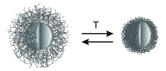
Figure 1: Schematic representation of the thermosensitive core-shell particles used in this study: The polymer chains are affixed to the surface of the core. Immersed in cold water the thermosensitive network will swell. The degree of swelling can be reduced by raising the temperature. At 32$\,{}^{o}$C a volume transition takes place in which most of the water is expelled from the network.

Recently, it has been demonstrated that suspensions of thermosensitive particles present excellent model systems for studying the flow of concentration suspensions for a quantitative comparison of the theory of Fuchs and Cates to experimental data [Fuchs and Ballauff (2005), Crassous et al. (2006a, 2008a)]. The particles consist of a solid core of polystyrene onto which a thermosensitive network of poly(N-isopropylacrylamide) (PNIPAM) is attached ([Crassous et al. (2006b, 2008b)], see Figure 1). The PNIPAM shell of these particles swells when immersed in cold water (below 32$\,{}^{o}$C). Water gets expelled at higher temperatures leading to a considerable shrinking. Thus, for a given number density the effective volume fraction $\phi_{eff}$ can be adjusted within wide limits by adjusting the temperature. Senff et al. (1999) were the first to demonstrate the use of these particles as model system for studying the dynamics in concentrated suspensions [Senff et al. (1999)]. Similar microgel particles have been used to study the dynamics of concentrated suspensions and the aging in these systems [Purnomo et al. (2006, 2007)]. The advantage of these systems over the classical hard sphere systems are obvious: Dense suspensions can be generated in situ without shear and mechanical deformation. Moreover, all previous history of the sample can be erased by raising the temperature and thus lowering the volume fraction to the fluid regime. Hence, subtle effects as e.g. aging can be studied by these systems in a nearly ideal fashion [Purnomo et al. (2006, 2007)]. Moreover, microgels can be used as models for pastes and gels in which the effective volume fraction of the particles exceeds unity by far [Seth et al. (2006)].

Previous investigations using dispersions of thermosensitive core-shell particles have demonstrated that mode-coupling theory is indeed able to model the flow curves as well as the linear viscoelasticity of concentrated suspensions [Crassous et al. (2006a, 2008a)]. In particular, this theory allows us to calculate $G^{\prime}$ and $G^{\prime\prime}$ as function of the frequency $\omega$ from data that have been obtained from the analysis of flow curves [Crassous et al. (2008a)]. However, a problem that restricted this comparison was crystallization due to the narrow size distribution of the particles. Crystallization presents a major obstacle since the rate of nucleation is rather fast for volume fractions even far below the volume fraction $\phi_{g}$ of glass transition ($\phi_{g}\approx 0.58$). The crystalline phase could be removed by shear melting and the fluid state could be super-cooled for a given time. The time window of nucleation, however, limited the experimental studies to frequencies and/or shear rates not too small [Crassous et al. (2006a, 2008a)]. A fully conclusive comparison of MCT with experimental data, however, requires that measurements extend down to the smallest frequencies and shear rates [Fuchs and Ballauff (2005), Crassous et al. (2008a)].

Here we present a full comparison of theory and experiment using a thermosensitive suspension having a slightly broader size distribution that prevents crystallization. Hence, all measurements can now be extended to very low shear rates or frequencies that may take hours without any disturbance by crystallization. It will be demonstrated that MCT provides indeed a full description of the rheological behavior of suspension under homogeneous flow. Special attention will be paid to shear banding [Callaghan (2008), Dhont and Briels (2008), Manneville (2008), Olmsted (2008)] and other effects that may come into play for concentrated suspensions [Isa et al. (2007)] and disturb the quantitative comparison of theory and experiment.

The paper is organized as follows: In the following section we give a brief survey of the main predictions of MCT. In particular, the equations used for the evaluation of data as well as the fit parameters necessary for a comparison of MCT with experimental data are discussed. For a extensive description of MCT the reader is deferred to a recent paper [Crassous et al. (2008a)]. After a section devoted to the description of the systems and the measurements, a comprehensive comparison of MCT with flow curves as well as with linear viscoelastic properties will given. A major focus is the low frequency and long time behavior which had not been accessible before. Special attention will be paid to the fact that MCT is capable of describing both the flow curves as well as $G^{\prime}$ and $G^{\prime\prime}$ as functions of frequency. A brief Conclusion will sum up the main findings.

2 Mode-coupling theory of flowing suspensions: Main predictions

The central points and main predictions of MCT and its generalization to flowing dispersions in the integration through transients (ITT) approach have recently been discussed in detail [Crassous et al. (2008a)]. Hence, it will suffice to discuss the points that will be used in the analysis of the experiments. Structural relaxation, which is the central topic of MCT, leads to internal relaxation processes with an intrinsic relaxation time $\tau$ that far exceeds the dilute limit Brownian diffusion time. The ITT-MCT approach to sheared fluids considers the effect of shear when the dressed Peclet or Weissenberg number $Pe=\dot{\gamma}\tau$ becomes appreciable, while the bare Peclet number $Pe_{0}=6\pi\eta_{s}R_{H}^{3}\dot{\gamma}/(k_{B}T)$ formed with the solvent viscosity $\eta_{s}$ and the hydrodynamic particle radius $R_{H}$ should be much lower than unity for the approach to hold.

The main point of the MCT of quiescent dispersions is the slowing down of the dynamics at the glass transition. Critical values for the particle concentration, the temperature or other thermodynamic control variables exist, where a glass transition separates fluid from yielding glassy states. In fluid states, a first Newtonian region is reached if the shear rate or the frequency is low enough; the Newtonian viscosity $\eta_{0}=\eta(\dot{\gamma}\to 0)$ is finite. Non-Newtonian flow, that is shear thinning, is observed at higher shear rates corresponding to a finite Weissenberg number Pe $\approx 1$. MCT recovers Maxwell’s relation $\eta_{0}\propto\tau$, so that the criterion $Pe\approx 1$ translates into $\eta_{0}\dot{\gamma}\approx G^{c}_{\infty}$, where $G^{c}_{\infty}=G^{\prime}(\omega\to 0)$ is the (zero-frequency) shear modulus at the glass transition. For glassy states at higher densities or interaction parameters, Newtonian flow is not observed anymore but the shear stress $\sigma$ is predicted to approach a plateau value for sufficiently low shear rates $\dot{\gamma}$; a dynamic yield stress follows $\sigma^{+}=\sigma(\dot{\gamma}\to 0)>0$. It corresponds to an infinite Newtonian viscosity.

A central point of MCT as applied to flowing suspensions [Fuchs and Cates (2002)] is shear melting: Finite shear rates will lead to a melting of the glass into a fluid. As a consequence of this, flow curves given by the shear stress $\sigma$ as function of the shear rate $\dot{\gamma}$ present well-defined states for a given volume fraction even above the glass transition. Hence, $\sigma(\dot{\gamma})$ is independent of the previous history of the sample, under the condition that the stationary long time limit has been achieved. Previous experimental studies strongly suggest that this central prediction of theory is found indeed [Crassous et al. (2006a, 2008a)]. However, in all previous experiments crystallization intervened at sufficiently low shear rates and this point is in need of further experimental elucidation.

In the following, the main equations used for the evaluation of the rheology data within MCT are briefly summed up. Within the schematic $F_{12}^{(\dot{\gamma})}$-model [Fuchs and Cates (2003)] Brownian motion of the particles is captured in terms of a density correlator $\Phi(t)$ which is normalized/initiated according to $\Phi(t\to 0)=1-\Gamma t$. MCT relates this correlation to the memory function $m(t)$ by a memory equation

$$\partial_{t}\Phi(t)+\Gamma\left\{\Phi(t)+\int_{0}^{t}dt^{\prime}\;m(t-t^{\prime})\;\partial_{t^{\prime}}\Phi(t^{\prime})\right\}=0\;.$$ (1)

The parameter $\Gamma$ describes the microscopic dynamics of the density correlator and will depend on structural and hydrodynamic correlations. The memory function describes stress fluctuations which become slower when approaching the volume fraction of the glass transition. In the $F_{12}^{(\dot{\gamma})}$-model the memory function is written as

$$m(t)=\frac{v_{1}\,\Phi(t)+v_{2}\,\Phi^{2}(t)}{1+\left(\dot{\gamma}t/\gamma_{c}\right)^{2}}.$$ (2)

This model, for the quiescent case $\dot{\gamma}=0$, had been suggested by Götze in 1984, [Götze (1984, 1991)] and describes the development of slow structural relaxation upon approaching a glass transition; it is reached by increasing the coupling vertices/ parameters $v_{1}$ and $v_{2}$ to their critical values $v_{1}^{c}=(2\lambda-1)/\lambda^{2}$ and $v_{2}^{c}=1/\lambda^{2}$, where the so-called exponent parameter $\lambda$ with $1/2\leq\lambda\leq 1$ parametrizes the (type-B) glass transition line. Under shear an explicit time dependence of the couplings in $m(t)$ captures the accelerated loss of memory by shear advection [Fuchs and Cates (2002, 2003, 2008)]. Shearing causes the dynamics to decay for long times, because fluctuations are advected to smaller wavelengths where small scale Brownian motion relaxes them. The parameter $\gamma_{c}$ sets the scale for the accumulated strain $\dot{\gamma}t$ to matter.

Equations (1, 2) will be used with the choice of vertices $v_{2}=v_{2}^{c}=2$ (corresponding to $\lambda=1/\sqrt{2}$), and $v_{1}=v_{1}^{c}+\varepsilon\,(1-f^{c})/f^{c}$, where $v_{1}^{c}=0.6258$. The critical glass form factor $f^{c}$, which takes the value $f^{c}=(1-\lambda)=0.293$ for this choice, describes the frozen-in structure obtained from $\Phi(t\to\infty,\varepsilon=0,\dot{\gamma}=0)=f^{c}$ at the glass transition in the absence of shear. The glass transition lies at $\varepsilon=0$, where the Newtonian viscosity diverges. Under shear, glass states are molten, but the transition still separates shear thinning fluid states, $\varepsilon<0$, where a Newtonian viscosity exists, from yielding glassy states $\varepsilon\geq 0$, where a dynamic yield stress $\sigma^{+}$ exists. The specific choice of this transition point is motivated by $(i)$ its repeated use in the literature, and $(ii)$ because it predicts a divergence of the viscosity at the glass transition, whose power is close to the one of the microscopic MCT calculation for short ranged repulsions:

$$\eta_{0}\propto\tau\propto\left(-\varepsilon\right)^{-\gamma}\;,\quad\mbox{with }\;\gamma=\gamma(\lambda=1/\sqrt{2})=2.34\;.$$

Within microscopic MCT for hard spheres using the Percus-Yevick structure factor $\gamma=2.46$ was found [Götze and Sjögren (1992)].

The correlator $\Phi(t)$ obtained by numerical solution of Eq. 1 may then be used to calculate the generalized shear modulus $g(t,\dot{\gamma})$ according to

$$g(t,\dot{\gamma})=v_{\sigma}\,\Phi^{2}(t)+\eta_{\infty}\;\delta(t-0+)\;.$$ (3)

The parameter $\eta_{\infty}$ characterizes a short-time high frequency viscosity and models viscous processes which require no structural relaxation. Together with $\Gamma$, it is the only model parameter affected by solvent mediated interactions. Steady state shear stress under constant shearing, and viscosity then follow via integrating up the generalized modulus:

$$\sigma=\eta\;\dot{\gamma}=\dot{\gamma}\;\int_{0}^{\infty}\!\!\!dt\;g(t,\dot{\gamma})=\dot{\gamma}\;\int_{0}^{\infty}\!\!\!dt\;v_{\sigma}\Phi^{2}(t)+\dot{\gamma}\;\eta_{\infty}\;.$$ (4)

When setting the shear rate $\dot{\gamma}=0$ in Eq. 2 so that the schematic correlator belongs to the quiescent equilibrium system, the frequency dependent moduli of the linear response framework follow from Fourier transforming:

$$G^{\prime}(\omega)+i\,G^{\prime\prime}(\omega)=i\,\omega\,\int_{0}^{\infty}\!\!\!dt\;e^{-i\,\omega\,t}\;g(t,\dot{\gamma}=0)=i\,\omega\,\int_{0}^{\infty}dt\;e^{-i\,\omega\,t}\;v_{\sigma}\left.\Phi^{2}(t)\right|_{\dot{\gamma}=0}+i\omega\,\eta_{\infty}\;$$ (5)

Because of the vanishing of the Fourier-integral in Eq. 5 for high frequencies, the parameter $\eta_{\infty}$ can be directly identified as high frequency viscosity:

$$\lim_{\omega\to\infty}G^{\prime\prime}(\omega)/\omega=\eta^{\omega}_{\infty}\quad,\;\mbox{with }\;\eta^{\omega}_{\infty}=\eta_{\infty}\;.$$ (6)

At high shear, on the other hand, Eq. 2 leads to a vanishing of $m(t)$, and Eq. 1 gives an exponential decay of the transient correlator, $\Phi(t)\to e^{-\Gamma\,t}$ for $\dot{\gamma}\to 0$. The high shear viscosity thus becomes

$$\eta^{\dot{\gamma}}_{\infty}=\lim_{\dot{\gamma}\to\infty}\sigma(\dot{\gamma})/\dot{\gamma}=\eta_{\infty}+\frac{v_{\sigma}}{2\,\Gamma}=\eta^{\omega}_{\infty}+\frac{v_{\sigma}}{2\,\Gamma}\;.$$ (7)

Eq. 7 connects the high-shear viscosity with the high-frequency limit of the viscosity in an analytical manner. Moreover, both $\eta^{\dot{\gamma}}_{\infty}$ and $\eta^{\omega}_{\infty}$ are accessible from experimental data and Eq. 7 provides an additional check for internal consistency of the fit within the frame of the schematic model. Representative solutions of the $F_{12}^{(\dot{\gamma})}$-model have been discussed recently [Crassous et al. (2008a), Fuchs and Cates (2003), Hajnal and Fuchs (2008)].

3 Experimental

The particles consist of a solid core of poly(styrene) onto which a network of crosslinked poly(N-isopropylacrylamide) (PNIPAM) is affixed [Crassous et al. (2006b, 2008b)]. The degree of crosslinking of the PNIPAM shell effected by the crosslinker N,N’-methylenebisacrylamide (BIS) was 2.5 Mol $\%$. The core-shell type PS-PNIPAM particles were synthesized, purified and characterized as described in [Dingenouts et al. (1998)]. Immersed in water the shell of these particles is swollen at low temperatures. Raising the temperature above 32$\,{}^{o}$C leads to a volume transition within the shell. Cryogenic transmission electron microscopy and dynamic light scattering have been used to investigate the structure and swelling of the particles [Crassous et al. (2006b, 2008b)]. Further experimental details on cryogenic transmission electron microscopy are given in [Crassous et al. (2006b)].
The average size and size distribution of the particles was determined with the CPS Disc Centrifuge from LOT, model DC 24000 in a aqueous glucose density gradient between 3 and 7$\,wt$% as medium at room temperature. The number-average diameter determined at 25$\,{}^{o}C$ is 131$\,nm$ and the standard deviation of the size distribution is 17 %.
Dynamic light scattering (DLS) was done with a Peters ALV 800 light scattering goniometer. The temperature was controlled with an accuracy of 0.1 ^oC. In the range of temperatures used for the measurements, $R_{H}$ could be linearly extrapolated between 6 and 25^oC ($R_{H}$ = -0.7796 $\cdot$T +102.4096 with T the temperature in ^oC) (see [Crassous et al. (2006a)]). Fig. 2b displays $R_{H}$ as the function of temperature. Moreover, this plot demonstrates that $R_{H}$ can obtained very precisely. Since the subsequent reduction of the data (see below) involves a scaling of the data by $R_{H}^{3}$, this fact is of great importance.

Density measurements have been made using a DMA-60 densiometer supplied by Paar (Graz, Austria). The density for the core-shell particles were determined as follows: $\varrho$ = 1.1184$\,g\,cm^{-3}$ at 25$\,{}^{o}C$, 1.1239$\,g\,cm^{-3}$ at 20$\,{}^{o}C$, 1.1246$\,g\,cm^{-3}$, at 18$\,{}^{o}C$ and 1.1259$\,g\,cm^{-3}$ at 17$\,{}^{o}C$. These densities can be described with the function $\varrho=6.800\cdot 10^{-7}\cdot T^{3}+1.129$ with the temperature T in ${}^{o}C$. In all experiments reported herein 5.10${}^{-2}\,mol\,L^{-1}$ KCl were added to the suspensions in order to screen the remaining electrostatic interactions caused by a few charges attached to the surface of the core particles. Previous studies have shown that this screening is fully sufficient. Thus, within the range of volume fractions under consideration here the thermosensitive particles can be regarded as hard spheres (see the discussion of this point in [Crassous et al. (2006a)]).

The flow behavior and the linear viscoelastic properties for the range of the low frequencies were measured with a stress-controlled rotational rheometer MCR 301 (Anton Paar), equipped with a Couette system (cup diameter: 28.929$\,mm$, bob diameter: 26.673$\,mm$, bob length: 39.997$\,mm$). For comparison the double gap geometry (inner cup diameter: 23.820$\,mm$, inner bob diameter: 24.660$\,mm$, outer bob diameter: 26.668$\,mm$, outer cup diameter: 27.590$\,mm$ and bob length: 40.00$\,mm$) was used as well. Measurements have been performed on 12$\,mL$ (Couette single gap geometry) and 4$\,mL$ (Couette double gap geometry) solution and the temperature was set with an accuracy of $\pm$ 0.05$\,{}^{o}$C. Deformation tests were done from a deformation of 0.1 to 100 % in the case of the dynamic deformation test with a logharitmic time ramp of 200 to 20$\,s$ at 1Hz. The shear stress $\sigma$ versus the shear rate $\dot{\gamma}$ (flow curve) was measured after a pre-shearing of $\dot{\gamma}=100\,s^{-1}$ for two minutes and a waiting time of 10$\,s$. The flow curves were obtained setting $\dot{\gamma}$ to a given value, first with increasing $\dot{\gamma}$ from $\dot{\gamma}=10^{-5}-10^{3}\,s^{-1}$ with a logarithmic time ramp from 1500 to 20$\,s$. Then after a waiting time of 10$\,s$ $\dot{\gamma}$ was decreased again.

The frequency dependence of the loss $G^{\prime\prime}$ and elastic $G^{\prime}$ moduli has been measured after a two minute pre-shear at a shear rate of 100$\,s^{-1}$ and 10$\,s$ waiting time for 1$\,\%$ strain from 10 to 10${}^{-4}\,Hz$ with a logarithmic time ramp from 20 to 1500$\,s$. The dependence upon the strain has been checked and confirmed that all the measurements were performed in the linear regime. $G^{\prime}$ and $G^{\prime\prime}$ at elevated frequencies were obtained using the Piezoelectric vibrator (PAV) [Crassous et al. (2005)] and cylindrical torsional resonator [Deike et al. (2001), Fritz et al. (2003)] supplied by the Institut für dynamische Materialprüfung, Ulm, Germany. The PAV was operated from 10 to 3000$\,Hz$. The solution is placed between two thick stainless steel plates. One remains static whereas the second is cemented to piezoelectric elements. The gap was adjusted with a 50$\,\mu\,m$ ring. A set of piezoelectric elements is driven by an ac voltage to induce the squeezing of the material between the two plates. The second set gives the output voltage. Experimental details concerning this instrument are given elsewhere [Crassous et al. (2005)]. The cylindrical torsional resonator (TR) used was operated at a single frequency (26$\,kHz$). The experimental procedure and the evaluation of data have been described recently [Deike et al. (2001), Fritz et al. (2003)].

4 Results and Discussion

4.1 Characterization

Recent work has shown that Cryo-TEM is a excellent tool for the analysis of the core-shell particles used for the present study [Crassous et al. (2006b, 2008b)] because this method allows us to visualize the particles in-situ, that is, directly in the aqueous suspension. Fig. 2 displays a micrograph of the suspension obtained by cryo-TEM. The core-shell structure of the particles is clearly visible as already demonstrated by previous work [Crassous et al. (2006b, 2008b)]. Since the polydispersity of the present suspension is considerably higher than the one of the dispersion used in our previous study [Crassous et al. (2008a)], the system does not crystallize anymore even if kept for a prolonged time at volume fractions above 50$\,\%$. However, Fig. 2 demonstrates that the suspension used here is still a well-defined model system. Hence, it can be used for a comprehensive comparison of experimental data with MCT. Attempts to suppress crystallization by mixing core-shell particles of slightly different size failed to produce reliable results since crystallization in these systems was found to be only slowed down but not suppressed totally.

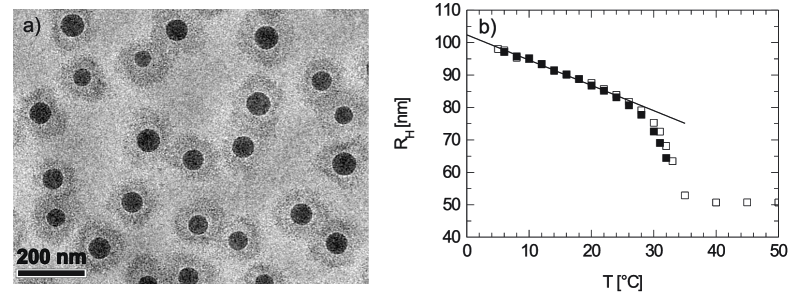
Figure 2: a) Cryogenic Transmission Electron Microscopy micrograph of the core-shell particles in water. b) Dynamic light scattering measurements of the latex at varius temperatures. Filled squares represent the hydrodynamic radius measured in aqueous 0.05$\,mol\,L^{-1}$ KCl, hollow squares measured in water. All rheological experiments presented here have been done using particles dissolved in aqueous 0.05$\,mol\,L^{-1}$ KCl solution [Crassous et al. (2006a, 2008a)]. In this way possible electrostatic interaction between the particles due to the residual charges affixed to the core particles can be screened totally. Below the volume transition the decrease of the hydrodynamic radius $R_{H}$ giving the outer boundary of the network is linear in very good approximation ($R_{H}$ = -0.7796 $\cdot$T +102.4096 with T being the temperature in ^oC; see solid line in graph).

The effective volume fraction $\phi_{eff}$ could not be calculated as for monodisperse particles by precise measurements of the hydrodynamic radius $R_{H}$, the core radius and the mass ratio of core and shell as done in [Crassous et al. (2008a)]. Unfortunately, polydispersity leads to an error which is too large and no meaningful data could be obtained. Furthermore, viscosity measurements in the dilute state and the use of the Batchelor-Einstein equation for the relative zero shear viscosity could not be applied because of the appreciable polydispersity, too. Therefore the effective volume fraction was obtained by comparing the relative viscosities at infinite shear rate with the monodisperse core-shell system used in [Crassous et al. (2008a)]. This will be discussed in further detail in conjunction with Fig. 6 below.

4.2 Reversibility of flow curves

Figure 3: a) Reversibility of the flowcurves for a 7.87$\,wt\%$ suspension at 12$\,{}^{\circ}C$ with two different geometries: Couette single gap - geometry (crosses) and double gap - geometry (squares). b) Reversibilty of the flowcurves by comparing jump experiments and the flowcurve (solid line) measured from higher to lower shear rates at 8.42$\,wt\%$ and 14.75${}^{\circ}C$. The steady state shear stress values of jumps from different shear rates to one as shown by the arrows in the graph are plotted for two examples: jump from 100$\,s^{-1}$ (full circle) to 0.000127$\,s^{-1}$ (full square) and jump from 0.0108$\,s^{-1}$ (hollow circle) to 0.000127$\,s^{-1}$ (full square). b) Inset: the same jumps are plotted time-dependent. The different jumps are plotted like followed: jump from 100$\,s^{-1}$ to 0.000127$\,s^{-1}$ (thick solid line) and jump from 0.0108$\,s^{-1}$ to 0.000127$\,s^{-1}$ (thick dashed line). The thin short dashed line in the inset represents the shear stress value at 0.000127$\,s^{-1}$ of the flowcurve for the same concentration and temperature.

A central prediction of MCT is the full reversibility of the flow curves, that is, of the shear stress $\sigma$ as the function of the shear rate $\dot{\gamma}$. This is evident for any volume fraction below the volume fraction $\phi_{g}$ of the glass transition. Here the system is ergodic and a well-defined steady state must be reached for sufficiently long time. This point is well borne out of all experiments done so far [Crassous et al. (2006a, 2008a)]. However, a totally different situation arises above $\phi_{g}$. In the glassy state, the suspension becomes non-ergodic and the flow curves may become ill-defined states. Hence, for concentrated suspensions of large non-Brownian particles dispersed in a highly viscous medium, the measured shear stress is found to be dependent on the previous history of the sample [Heymann and Aksel (2007)]. MCT, however, predicts that shear melting sets in at any finite shear rate $\dot{\gamma}$. Therefore, shear flow restores the ergodicity in the system and thermal motion of the spheres can erase all traces of the previous deformations of the sample if flow is applied over a sufficiently long time interval. Two types of experiments need to be done to explore these basic principles in further detail:

i) Each data point giving $\sigma(\dot{\gamma})$ must be independent regardless of the shear history. Thus, flow curves $\sigma(\dot{\gamma})$ should be fully reversible regardless whether the data are taken by increasing rate or decreasing the shear rate. The reversibility of the flow curves has already been demonstrated in previous work. However, the suspensions analyzed previously [Crassous et al. (2006a, 2008a)] began to crystallize during the long measurements needed for exploring the dynamics at smallest shear rates $\dot{\gamma}$. To overcome this problem, the present system is sufficiently polydisperse, crystallization is suppressed. Fig. 3 displays the resulting flow curves down to $Pe_{0}=10^{-6}$. The onset of a plateau is clearly seen. Additional experiments with long waiting times demonstrated that crystallization does not occur in the present system. Moreover, Fig. 3a points to another important fact: $\sigma(\dot{\gamma})$ is entirely independent of the geometry of the rheometer used for studying the flow behavior. Fig. 3a demonstrates this fact by overlaying the resulting $\sigma(\dot{\gamma})$ obtained from a single gap and double gap Couette geometry. If shear banding would play any role [Callaghan (2008), Dhont and Briels (2008), Manneville (2008), Olmsted (2008)], the resulting $\sigma(\dot{\gamma})$ should be different and depend definitely on the width of the gap of the instrument. The difference in curvature for the two experiment geometries would have resulted in different onsets of shear banding. Also, shear banding in the double-gap Couette system would have resulted in a complex interplay of instabilities in the two gaps. None of this is observed here.

ii) The full reversibility of the flow curves are demonstrated also by a second type of experiment (Fig. 3b): Here a stationary state is first obtained for a given shear rate $\dot{\gamma}$. Then a much lower shear rate is adjusted and the resulting shear stress is monitored as a function of time. Fig. 3b shows that $\sigma(\dot{\gamma})$ converges to the stationary value measured previously (solid line in Fig. 3b). The inset displays the evolution of $\sigma(\dot{\gamma})$ with time. Evidently, a long time may be needed until the stationary value is reached. However, all data demonstrate that the full reversibility of $\sigma(\dot{\gamma})$ is fully supported by our experiment also above the glass transition. One of the central predictions is thus fully corroborated. Deviations observed previously [Crassous et al. (2008a)] were solely due to crystallization of the sample which is suppressed in the present system. In this way flow curves may to a certain extent be compared to thermodynamic results, they are fully independent of the path leading to a given state.

A point to be considered further is the transition from the linear to the non-linear viscoelastic regime in the glassy regime. Fig. 4 displays $G^{\prime}$, $G^{\prime\prime}$ as well as $\sigma$ for different deformations at a rate of 1 Hz. The data show that the linear regime is preserved up to a strain of nearly 10$\%$. Moreover, $G^{\prime}\gamma$ measured for different strains $\gamma$ coincides directly with the measured stress $\sigma$. Hence, within this range of $\gamma$, the glassy suspensions behaves as a homogeneous solid as expected. Again, shear banding or possible inhomogeneities within the gap should disturb this type of measurement. Fig. 4 demonstrates that this is not seen. Obviously, these experiments are not fully sufficient to rule out shear banding entirely. However, the good agreement between two entirely different types of experiments with theory to be discussed further below points clearly to the fact that shear banding does not disturb the measurements reported here.

Beyond a strain of ca. 10 $\%$, shear melting of the glass starts and the measured stress $\sigma$ is considerably lower than the value calculated from $G^{\prime}$. Fig. 4 indicates that the linear viscoelastic regime is extended over a sufficiently large range of deformations.

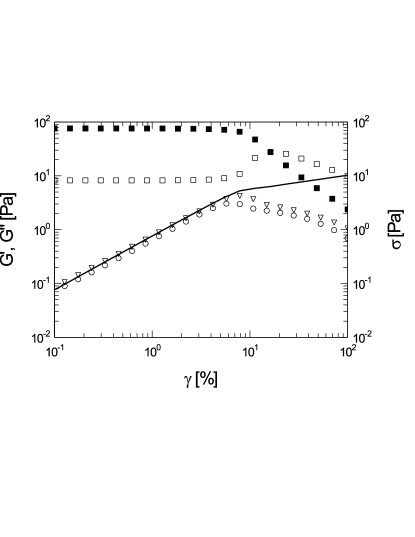
Figure 4: Comparison of the dynamic strain sweep at 1$\,Hz$ (G’: filled squares, G” open squares, $\sigma$ solid line) and a continuous strain sweep with two different measurement times for each point (20$\,s$ per point: triangles down and 200$\,s$ per point: circles) for a 8.90$\,wt\%$ suspension at 17$\,{}^{\circ}$C ($\phi_{eff}$ = 0.627).

4.3 Comparison with mode coupling theory: Schematic model

A thorough comparison of ITT-MCT to experimental data must be related not only to the flow curves discussed in the previous section but also to data obtained for the linear viscoelasticity, that is for $G^{\prime}$ and $G^{\prime\prime}$ as function of the frequency $\omega$. A previous comparison [Crassous et al. (2008a)] has demonstrated that both sets of data can indeed be described by a generalized modulus $g(t,\dot{\gamma})$ as introduced in the section Theory. However, at smallest Pe₀ crystallization intervened and the comparison was restricted to intermediate to high shear rates/frequencies. Crystallization is suppressed for the present system and a fully quantitative comparison of theory and experiment now becomes possible down to $Pe_{0}\approx 10^{-8}$ in case of the flow curves. $G^{\prime}$ and $G^{\prime\prime}$ can be obtained down to $Pe_{\omega}\approx 10^{-6}$. Here, the frequency dependent Peclet (or Deborrah) number, defined as $Pe_{\omega}=6\pi\eta_{s}R_{H}^{3}\omega/(k_{B}T)$, compares the frequency with the time it takes a particle to diffuse its radius $R_{H}$ at infinite dilution. At high densities, structural relaxation shows up at Pe${}_{\omega}\ll 1$ .

Figure 5: Left column: Reduced flow curves for different volume fractions (graphs in left column a, c, e, g and i). Hollow squares represent the ”‘up”’ curve from low to high shear rates, filled squares represent the ”‘down”’curve from high to low shear rates. The solid lines are the results of the schematic model, the dashed line represent the pseudo power law behavior (see Table 2).Right column: Reduced frequency dependent moduli for different volume fractions (graphs b, d, f, h and j in right column). Full symbols/solid lines represent G’, hollow symbols/dashed lines represent G”. Squares mark the data points obtained by the Physica MCR 301, circles with the PAV, triangles up with the TR, the thick lines are the results of the schematic model, the thin lines the results of the microscopic model.Graphs in one row represent the continuous and dynamic measurements at one volume fraction. a and b were measured at 8.90$\,wt\%$ and 25$\,{}^{\circ}$C $\phi_{eff}$ = 0.530 , c and d were measured at 7.87$\,wt\%$ and 18$\,{}^{\circ}$C (circles) $\phi_{eff}$ = 0.595 , e and f at 8.90$\,wt\%$ and 20$\,{}^{\circ}$C $\phi_{eff}$ = 0.616 , g and h at 8.90$\,wt\%$ and 19$\,{}^{\circ}$C $\phi_{eff}$ = 0.625 , and i and j at 8.90$\,wt\%$ and 17$\,{}^{\circ}$C $\phi_{eff}$ = 0.627 .

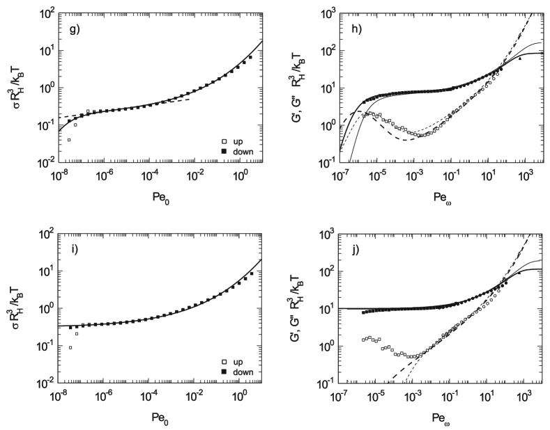
Figure 5: Continued.

In the following we shall compare the experimental flow curves and $G^{\prime}$ and $G^{\prime\prime}$ with theory for a given effective volume fraction $\phi_{eff}$. Fig. 5 gives this comparison for five different effective volume fractions. On the left-hand side the flow curves $\sigma(\dot{\gamma})$ are presented as function of the bare Peclet number $Pe_{0}$, on the right-hand side $G^{\prime}$ and $G^{\prime\prime}$ are displayed as the function of Pe_ω, now calculated with the respective frequencies $\omega$. Table 1 gathers the respective volume fractions together with the other experimental conditions. Note that $G^{\prime}$ and $G^{\prime\prime}$ have been obtained over nearly 7 orders of magnitude in frequency by combining a Couette rheometer (single gap, double gap) with the PAV and the torsional resonator.

The generalized shear modulus $g(t,\dot{\gamma})$ (cf. Eq. 3) presents the central theoretical quantity used in this fit. Within the schematic model, the vertex prefactor $v_{\sigma}$ is kept as a shear-independent quantity. It can easily be obtained from the stress and modulus magnitudes. Hydrodynamic interactions enter through $\eta_{\infty}$, which can be obtained from measurements done at high frequencies, and through $\Gamma$, which can be obtained via Eq. 7 from measurements done at high shear rates. Given these three parameters, both the shapes of the flow curves as well as the shapes of the moduli $G^{\prime}$ and $G^{\prime\prime}$ may be obtained as function of the two parameters $\varepsilon$ and $\dot{\gamma}/\gamma_{c}$. The former sets the separation to the glass transition and thus (especially) the longest relaxation time, while the latter tunes the effect of the shear flow on the flow curve. The characteristic changes of the shapes of the steady stress and the moduli are dominated by $\varepsilon$ and $\dot{\gamma}/\gamma_{c}$.

c	T	$\phi_{eff}$	$\varepsilon$	$v_{\sigma}$	$\Gamma$	$\gamma_{c}$	$\eta_{\infty}$ = $\eta_{\infty}^{\omega}$	$\eta_{\infty}^{\dot{\gamma}}$	$\sigma_{0}$	$\eta_{0}$
$\left[wt\%\right]$	$\left[{}^{o}C\right]$			$\left[\frac{k_{B}T}{R_{H}^{3}}\right]$	$\left[\frac{D_{0}}{R_{H}^{2}}\right]$		$\left[\frac{k_{B}T}{D_{0}R_{H}}\right]$	$\left[\frac{k_{B}T}{D_{0}R_{H}}\right]$	$\left[\frac{k_{B}T}{R_{H}^{3}}\right]$	$\left[\frac{k_{B}T}{D_{0}R_{H}}\right]$
8.90	25	0.530	-0.072000	18	20	0.0845	0.2250	0.6750	-	1.1345$\cdot 10^{1}$
7.87	18	0.595	-0.003500	48	50	0.1195	0.2400	0.7200	-	7.7439$\cdot 10^{3}$
8.90	20	0.616	-0.000420	70	80	0.1414	0.3938	0.8313	-	1.0177$\cdot 10^{6}$
8.90	19	0.625	-0.000170	85	90	0.1491	0.4250	0.8972	-	9.1562$\cdot 10^{6}$
8.90	17	0.627	0.000021	115	120	0.1622	0.4313	0.9104	3.3193$\cdot 10^{-1}$	-

Table 1: Experimental parameters (concentration $c$, temperature $T$ and calculated $\phi_{eff}$) of the measurements shown in Fig. 5. The fit parameter $v_{\sigma}$, $\Gamma$, $\gamma_{c}$ and $\eta_{\infty}$ of the $F_{12}^{\dot{\gamma}}$ model as well as the calculated values $\eta_{\infty}^{\dot{\gamma}}$, $\sigma_{0}$ and $\eta_{0}$ are written in terms of the respective normalization.

The fitting of the data was done as follows: All measured quantities, namely $\sigma$, $G^{\prime}$, and $G^{\prime\prime}$ were converted to the respective dimensionless quantities by multiplication with $R_{H}^{3}/k_{B}T$ where $R_{H}$ is the hydrodynamic radius at the respective temperature. Previous work has demonstrated that the effective volume fraction deriving from $R_{H}$ is the only decisive thermodynamic parameter [Crassous et al. (2006a, 2008a)]. As already discussed above, $\dot{\gamma}$ and $\omega$ are converted by $6\pi\eta_{s}R_{H}^{3}/k_{B}T$ to the respective Peclet numbers.

Evidently, both the reduced moduli, the Pe number, and the packing fraction depend on the effective particle volume $R_{H}^{3}$. Therefore, this quantity must be measured with utmost precision. In our polydisperse sample, actually a distribution of values $R_{H}^{3}$ exists, whose variance we determined by disc centrifugation at low concentration. It is important to note, however, that the size distribution does not change with temperature. Moreover, in our experiments close to the glass transition, we may assume the size distribution to be (almost) density independent. Therefore, we have $R_{H}^{3}(T)$ as single experimental control parameter, whose small change upon varying temperature $T$ drives the system through the glass transition (see also the discussion of Fig. 6).

Subsequently, the fit procedure is started at the smallest volume fraction and a trial value for the separation parameter $\varepsilon$ is chosen. This fit can be done very accurately since the resulting reduced moduli depend very sensitively on $\varepsilon$. Once the overall shape of both the reduced stress $\sigma R_{H}^{3}/k_{B}T$ and of the reduced storage and loss modulus has been reproduced by a proper choice of $\varepsilon$, the vertex parameter $v_{\sigma}$ is obtained. For lower volume fraction the crossing point of $G^{\prime}$ and $G^{\prime\prime}$ may be used, near the glassy state the plateau value of $\sigma$ and $G^{\prime}$ can be used. Note that in all steps both sets of data, that is, the flow curves as well as $G^{\prime}$ and $G^{\prime\prime}$ must be fitted with the same $v_{\sigma}$. Next $\Gamma$ is determined from the dynamic data which are fully described with this choice of parameters. Given $\gamma$, the parameter $\gamma_{c}$ (see Eq. 2) is chosen so that the experimental flow curves are matched by theory. Then $\eta_{0}$, $\sigma_{0}$ and $\eta_{\infty}^{\dot{\gamma}}$ can be calculated. The results of these fits are gathered in Table 1. We reiterate that the final set of parameters must lead to a description of both the flow curves as well as of the dynamic data. This requirement stresses the connection of the equilibrium structural relaxation at the glass transition to the non-linear rheology under strong flow, which is one of the central points of the ITT-MCT approach.

Fig. 5 demonstrates that the rheological behavior of a non-crystallizing colloidal can be modeled in a highly satisfactory manner by five parameters that display only a weak dependence on the effective volume fraction of the particles. Increasing the effective packing fraction drives the system toward the glass transition, viz. $\varepsilon$ increases with $\phi_{eff}$. Stress magnitudes (measured by $v_{\sigma}$) also increase with $\phi_{eff}$, as do high frequency and high shear viscosities; their difference determines $\Gamma$. The strain scale $\gamma_{c}$ remains around the reasonable value 10$\,\%$. In spite of the smooth and small changes of the model parameters, the $F_{12}^{\dot{\gamma}}$-model achieves to capture the qualitative change of the linear and non-linear rheology. The measured Newtonian viscosity increases by a factor around $10^{5}$. The elastic modulus $G^{\prime}$ at low frequencies is utterly negligible at low densities, while it takes a rather constant value around $10k_{B}T/R^{3}_{H}$ at high densities. An analogous observation holds for the steady state shear stress $\sigma(\dot{\gamma})$, which at high densities takes values around $0.3k_{B}T/R^{3}_{H}$ when measured at lowest shear rates. For lower densities, shear rates larger by a factor around $10^{7}$ would be required to obtain such high stress values.

At volume fractions around 0.5 the suspension is Newtonian at small $Pe_{0}$ (see Fig. 5). Evidently, these flow curves are fully reversible since the suspension is still in the fluid regime. The schematic model provides a perfect fit. Moreover, theory demonstrates in full agreement with experiment that the high-shear viscosities measured in shear flow and the high-frequency viscosities measured in the linear viscoelastic regime do not agree. As is evident from Eq. 7, both $\eta_{\infty}^{\dot{\gamma}}$ and $\eta_{\infty}^{\omega}$ are related by Eq. 7 and the Cox-Merz rule does not hold for suspensions as expected. Approaching the glass transition leads to a characteristic S-shape of the flow curves and the Newtonian region becomes more and more restricted to the region of smallest $Pe_{0}$. Concomitantly, a pronounced minimum in $G^{\prime\prime}$ starts to develop, separating the slow structural relaxation process from faster, rather density independent motions, while $G^{\prime}$ exhibits a more and more pronounced plateau. At the highest densities (Fig. 5 panels i and j), the theory would conclude that a yielding glass is formed, which exhibits a finite elastic shear modulus (elastic constant) $G_{\infty}=G^{\prime}(\omega\to 0)$, and a finite dynamic yield stress, $\sigma^{+}=\sigma(\dot{\gamma}\to 0)$. The experiment shows, however, that small deviations from this glass like response exist at very small frequencies and strain rates. Description of this ultra-slow process requires extensions of the present ITT-MCT [Crassous et al. (2008a)], where additional physical mechanisms for stress relaxation need to be considered that are neglected here.

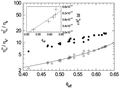
Figure 6: Relative viscosities in dependence of the effective volume fraction for a monodisperse latex [Crassous et al. (2008a)] (circles) and the polydisperse latex (this work; squares). The hollow symbols show the high frequency viscosities, the filled symbols the high shear viscosities. The relative high frequency viscosity $\eta_{\infty}^{\omega}$ can be described by Lionberger-Russel - equation (see Eq. 4.22 in Lionberger and Russel (1994)) with a reduced effective volume fraction of 11.95$\,\%$. Assuming the same relation for the polydisperse latex under consideration here, $\eta_{\infty}^{\omega}$ was used to determine the effective volume fractions. The $\phi_{eff}$ obtained by this way are plotted in the inset versus the concentration $c$ [$g\cdot mL^{-1}$] times the cubed hydrodynamic radius $R_{H}^{3}$ [$m^{3}$]. The solid line represents the linear scaling of effective volume fraction and $c\cdot R_{H}^{3}$ with a slope of 9.77$\cdot$ 10${}^{-17}\,g$ and a intercept of zero. As a further check, the high-shear viscosities are plotted as well as a function of $\phi_{eff}$. The filled circles show this quantity for the narrowly distributed latex [Crassous et al. (2008a)] whereas the filled squares denote the repsective quantities for the present system. Good agreement is seen thus corroborating the present way of determining $\phi_{eff}$.

4.4 Power laws

Often power-law shear thinning is discussed, when the viscosity is plotted as function of shear rate instead of the flow curves, viz. stress versus shear rate. For fluid states, the double logarithmic presentation in Fig. 5 shows characteristically S-shaped flow curves, which have a point of inflection. Clearly, this flow curve being a more sensitive presentation as the usual $\eta(\dot{\gamma})$-plots rules out the existence of a true power law behavior, which should show up as a straight line in the double logarithmic plot. Yet, at the point of inflection of the S-curve, and closely around it, a pseudo-power law may exist. Here $\eta(\dot{\gamma})\sim\dot{\gamma}^{(p-1)}$, where $p$ is the slope of the tangent in the flow curve at the inflection point, $p=d\ln{\sigma}/d\ln{\dot{\gamma}}$. These tangents are indicated by dashed straight lines in the panels of Fig. 5. The pseudo-power law that corresponds to the one in the viscosity can describe the flow curve over more than two decades in shear rate. The exponents $p$ (see Table 2) change with density, and can be computed within the schematic model [Hajnal and Fuchs (2008)]. Nevertheless, Fig. 5 shows clearly that the description by power laws is by far inferior to the one provided by MCT.

4.5 Effective volume fraction

As already lined out in the section Experimental, the higher polydispersity of the suspension used here suppresses crystallization. On the other hand, the precise determination of the volume fractions at which crystallization occurs leads to a precise determination of the effective volume fractions $\phi_{eff}$ [Cheng et al. (2002)]. This fact has been used in our previous study using a narrowly distributed thermosensitive system [Crassous et al. (2006a, 2008a)]. In this way the zero-shear viscosity as well as the high-frequency and the high-shear viscosities could be obtained as the function of $\phi_{eff}$. The effective volume fraction $\phi_{eff}$ may in principle be determined from the mass balance as lined out in previous studies [Crassous et al. (2006a, 2008a)]. However, the error in this determination turned out to be of appreciable magnitude. Hence, we followed the suggestion of Cheng et al. (2002) and compared the high-frequency viscosities of the narrowly distributed system studied previously [Crassous et al. (2008a)] with the respective values determined directly for the present system. Fig. 6 displays the resulting dependence of the high-frequency viscosities (hollow symbols) and the high-shear viscosities (filled symbols) on $\phi_{eff}$. The relative high frequency viscosity $\eta_{\infty}^{\omega}$ can be described by equation 4.22 in [Lionberger and Russel (1994)] with a reduced effective volume fraction of 11.95$\,\%$ as opposed to the actual value of $\phi_{eff}$, the volume transition neglegting a partial draining. The marked reduction of the volume fraction at high frequencies has already been detected in a previous study of a similar system [Deike et al. (2001)] and was explained by a partial draining of the thermosensitive network. The resulting correlation between the effective volume fractions and $\eta_{\infty}^{\omega}$ of the narrowly distributed systems can then be used to determine $\phi_{eff}$ of the present system. The values thus obtained are gathered in Table 1. Moreover, the inset of Fig. 6 demonstrates that there is a linear relationship between these $\phi_{eff}$ and $cR_{H}^{3}$ as discussed above. A further check of the data is provided by a comparison of the high-shear viscosities $\eta_{\infty}^{\dot{\gamma}}$ for both systems. Fig. 6 demonstrates that both sets of data agree within the given limits of error. This fact demonstrates that the present procedure leads to reliable values of $\phi_{eff}$.

4.6 Microscopic MCT calculations

While schematic models provide a handy description of the universal features close to the glass transition and the shear melting of glasses, the microscopic formulation of ITT-MCT actually aims to predict from first principles the nonlinear rheology starting with the underlying particle interactions; see the Appendix for a short summary. Because of the anisotropy of the structure under shear, it has not been possible yet to solve the ITT-MCT equations without approximations. Only solutions of schematic or isotropically averaged models are available. Yet, without shear the equations of quiescent MCT [Götze 1991] can be solved readily and can be compared to the frequency dependent moduli within linear response regime. This has been done considering the monodisperse system in Ref. [Crassous et al. (2008a)], and after determination of the effective packing fraction we could perform identical calculations for the polydisperse system; see Ref. [Crassous et al. (2008a)] for details of the calculation which use the Percus-Yevick approximation to the structure factor of hard spheres. Here, of course the simplification to do monodisperse MCT calculations to compare with the measurements in the polydisperse system adds to the errors in the comparisons. The adjustable parameters, mainly the effective collective short time diffusion coefficient and the effective packing fraction setting the separation to the glass transition are reported in Table 2. Quite good agreement with the data can be achieved, with parameters that vary regularly with density and take quite reasonable values. Interestingly, the polydisperse system has larger moduli by a factor around two than the monodisperse system at the same effective packing fraction.

$c$	$T$	$\phi_{eff}$	$\varepsilon$	$\phi$	$c_{y}$	$D_{s}/D_{0}$	$p$
$[wt\%]$	$[^{o}C]$
8.90	25	0.530	-0.10000	0.4643	2.3	0.3	0.631
7.87	18	0.595	-0.00794	0.5118	2.3	0.3	0.248
8.90	20	0.616	-0.00126	0.5153	2.3	0.3	0.117
8.90	19	0.625	-0.00100	0.5154	3.0	0.3	0.0852
8.90	17	0.627	0.00158	0.5167	3.5	0.3

Table 2: Experimental parameters (concentration $c$, temperature $T$ and experimental effective volume fraction $\phi_{eff}$ with $\phi_{g}$ = 0.58. The parameters of the microscopic calculations (separation parameter $\varepsilon$, volume fraction $\phi$ with $\phi_{g}$ = 0.5159, $c_{y}$ and $D_{S}/D_{0}$, where $D_{0}=k_{B}T/(6\pi\eta_{s}R_{H})$), as shown in Fig. 5 are listed here. Furthermore, the power law exponents $p$ from the dashed lines in the flowcurves of Fig. 5 are given in this table.

5 Conclusion

The fluid-to-glass transition in colloidal suspensions leads to characteristic changes of the flow curves and concomitantly of $G^{\prime}$ and $G^{\prime\prime}$ as the function of frequency. Here we demonstrated that both sets of data can be quantitatively modeled by a single generalized modulus $g(t,\dot{\gamma})$. Moreover, $g(t,\dot{\gamma})$ can be fully described by mode-coupling theory (MCT). Hydrodynamic interaction enters only through the high-shear and the high-frequency viscosities $\eta_{\infty}^{\dot{\gamma}}$ and $\eta_{\infty}^{\omega}$, respectively. MCT demonstrates that the latter quantities are not identical but closely related to each other (see the discussion of Eq. 7). Small deviations between data and theory are only seen for $G^{\prime\prime}$ in the immediate vicinity of the glass volume fraction and only at the lowest Peclet numbers $Pe_{\omega}$. This finding can be assigned to a very slow relaxation that is not captured by MCT.

Appendix

The ITT approach, which generalizes the MCT of the glass transition to colloidal dispersions under stationary shear [Fuchs and Cates (2002); ibid. (2008)], consists of equations of motion for a density correlator $\Phi_{\bf q}(t)$ which describes structural rearrangements, and approximated Green-Kubo formulae relating stress relaxation to decay of density fluctuations. The approach was described in [Crassous et al. (2008a)], and the used equations can be summarized as follows.

The density correlator obeys an equation of motion containing a retarded friction kernel which arises from the competition of particle caging and shear advection of fluctuations

$$\partial_{t}\Phi_{\bf q}(t)+\Gamma_{\bf q}(t)\;\left\{\Phi_{\bf q}(t)+\int_{0}^{t}dt^{\prime}\;m_{{\bf q}(t^{\prime})}(t-t^{\prime})\;\partial_{t^{\prime}}\,\Phi_{\bf q}(t^{\prime})\right\}=0\;.$$ (8)

with the advected wavector ${\bf q}(t)$, whose component along the gradient direction varies with time, $q_{y}(t)=q_{y}(0)-\dot{\gamma}t\;q_{x}$ because of the affine component of the particle motion; while $q_{x}$ and $q_{z}$ remain time-independent. The density correlator is normalized $\Phi_{\bf q}(t=0)=1$ . Its initial decay is described by $\Gamma_{\bf q}(t)=D_{s}q^{2}(t)/S_{q(t)}$, with $D_{s}$ the collective short time diffusion coefficient, which may depend on hydrodynamic interactions, and thus differ from the Stokes-Einstein-Sutherland value. The equilibrium structure factor $S_{q}$, encodes the particle interactions and introduces the experimental control parameters like density and temperature. The generalized friction kernel $m_{{\bf q}^{\prime}}(t)$, which is an autocorrelation function of fluctuating stresses, is approximated from the structural rearrangements captured in the density correlators

$$m_{\bf q^{\prime}}(t)=\frac{1}{2N}\sum_{\bf k}\frac{S_{q^{\prime}(t)}\,S_{k}\,S_{p}}{{q^{\prime}}^{2}(t)\;{q^{\prime}}^{2}}\;V_{{\bf q}^{\prime}{\bf k}{\bf p}}(t)\,V_{{\bf q}^{\prime}{\bf k}{\bf p}}(0)\;\Phi_{\bf k}(t)\;\Phi_{\bf p}(t)\;,$$ (9)

where the vertices are given by the equilibrium structure factor

$$V_{\bf qkp}(t)={\bf q}(t)\cdot\left({\bf k}(t)\,nc_{k(t)}+{\bf p}(t)\,nc_{p(t)}\right)\;\delta_{{\bf q},{\bf k}+{\bf p}}\;,$$ (10)

with $n$ the particle density, and $c_{k}$ the Ornstein-Zernicke direct correlation function $c_{k}=(1-1/S_{k})/n$. Similarly, the generalized shear modulus is approximated assuming that stress relaxations can be computed from integrating the transient density correlations

$$g(t,\dot{\gamma})=\frac{k_{B}T}{2}\int\!\!\frac{d^{3}k}{(2\pi)^{3}}\;\frac{k_{x}^{2}k_{y}k_{y}(-t)}{k\,k(-t)}\;\frac{S^{\prime}_{k}S^{\prime}_{k(-t)}}{S^{2}_{k}}\;\Phi^{2}_{{\bf k}(-t)}(t)\;,$$ (11)

where $S^{\prime}_{k}=\partial S_{k}/\partial k$.

The schematic $F_{12}^{(\dot{\gamma})}$-model described above follows from a simplification of these equations. It mimicks using $v_{1}$ and $v_{2}$ the increase of the vertices $V_{{\bf q}^{\prime}{\bf k}{\bf p}}$ with sharpening structural correlations in $S_{q}$ , which captures the cage effect causing a glass transition [Götze (1991), Götze and Sjögren (1992)]. It mimicks with $1/(1+(\dot{\gamma}t/\gamma_{c})^{2})$ the shear-driven decorrelation, which can be recognized from the vanishing of the memory kernel at long times under shear: $m_{{\bf q^{\prime}}}(t\dot{\gamma}\gg 1)=0$ and $m_{{\bf q^{\prime}}}(t)-m_{q}(t)^{(\dot{\gamma}=0)}={\cal O}((\dot{\gamma}t)^{2})$ in the microscopic ITT equations [Fuchs and Cates (2002)]. Without shear, $\dot{\gamma}\equiv 0$, Eqs. (8-11) become the familiar MCT equations which can readily be solved after discretization, as has been done in previous studies [Crassous et al. (2008a)]. The thin dashed lines in Fig. 5 labeled microscopic model result from these calculations, with parameters listed in Table 2. But under shear the equations become anisotropic and require more severe approximations, like for example using the simple schematic $F_{12}^{(\dot{\gamma})}$-model.

In detail, the equations were solved for a dispersion of monodisperse hard spheres with structure factor $S_{k}$ taken from the Percus-Yevick approximation. The wavevector integrals in the microscopic model Eqs. (8-12) were discretized according to Ref. [Crassous et al. (2008)] using $M=600$ wavevectors chosen from $k_{\rm min}=0.05/R_{H}$ up to $k_{\rm max}=59.95/R_{H}$ with separation $\Delta k=0.1/R_{H}$. Time was discretized with initial step-width $dt=2\,10^{-7}R_{H}^{2}/D_{s}$, which was doubled each time after 400 steps. Because the first principles calculations carry quantitative errors, which would mask the qualitative comparison, two adjustments of parameters were performed. The magnitude of the linear modulus is too small in theory by a factor $c_{y}$ which is included in Table 2. The computed position of the glass transition is also somewhat to small, $\phi_{g}=0.5159$ in MCT relative to $\phi_{g}=0.58$ in experiment. Therefore the relative separation, $\varepsilon=(\phi-\phi_{g})/\phi_{g}$ was used as adjustable parameter quantifying the distance to the glass transition; the fitted values are also contained in Table 2.

References

Banchio, A. J., J. Bergenholtz, G. Nägele, “Viscoelasticity and generalized Stokes-Einstein relations of colloidal dispersions.”, J. Chem. Phys. 111, 8721 (1999).

Callaghan, P. “Rheo NMR and shear banding.” Rheol. Acta, 47, 243 (2008).

Cheng, Z., J. Zhu, P. M. Chaikin, S.-E. Phan, W. B. Russel, ”‘Nature of the divergence in low shear viscosity of colloidal hard-sphere dispersions”’, Phys. Rev. E 65, 041405 (2002).

Crassous, J. J., R. Regisser, M. Ballauff and W. Willenbacher, ”‘Characterization of the viscoelastic behavior of complex fluids using the piezoelastic axial vibrator”’, J. Rheol. 49, 851 (2005).

Crassous, J. J., M. Siebenbürger, M. Ballauff, M. Drechsler, O. Henrich, M. Fuchs, “Thermosensitive core-shell particles as model systems for studying the flow behavior of concentrated colloidal dispersions”, J. Chem. Phys. 125, 204906 (2006a).

Crassous, J. J., M. Ballauff, M. Drechsler, J. Schmidt, Y. Talmon, “Imaging the Volume Transition in thermosensitive Core-Shell Particles by Cryo-Transmission Electron Microscopy” Langmuir 22, 2403 (2006b).

Crassous, J. J., M. Siebenbürger, M. Ballauff, M. Drechsler, D. Hajnal, O. Henrich, M. Fuchs, “Shear stresses of colloidal dispersions at the glass transition in equilibrium and in flow”, J. Chem. Phys. 128, 204902 (2008a).

Crassous, J. J., A. Wittemann, M. Siebenbrger, M. Schrinner, M. Drechsler, M. Ballauff, “Direct Imaging of Temperature-Sensitive Core-Shell Latexes by Cryogenic Transmission Electron Microscopy”, Colloid Polym. Sci. 286, 805 (2008b).

Deike, I., M. Ballauff, N. Willenbacher, A. Weiss, ”‘Rheology of thermosensitive latex particles including the high-frequency limit”’, J. Rheol. 45, 709 (2001).

Dhont J, Briels W “Gradient and vorticity banding.” Rheol. Acta 47, 257 (2008).

Dingenouts, N., Ch. Norhausen and M. Ballauff, ”‘Observation of the Volume Transition in Thermosensitive Core-Shell Latex Particles by Small-Angle X-ray Scattering”’, Macromolecules, 31, 8912 (1998).

Fritz, G., W. Pechhold, N. Willenbacher and J. W. Norman, ”‘Characterizing complex fluids with high frequency rheology using torsional resonators at multiple frequencies”’, J. Rheol. 47, 303 (2003).

Fuchs, M. and M. E. Cates, ”‘Theory of Nonlinear Rheology and Yielding of Dense Colloidal Suspensions”’, Phys. Rev. Lett. 89, 248304 (2002).

Fuchs, M. and M. E. Cates, ”‘Schematic models for dynamic yielding of sheared colloidal glasses”’, Faraday Disc. 123, 267 (2003).

Fuchs, M. and M. Ballauff, “Flow curves of dense colloidal suspensions: Schematic model analysis of the shear-dependent viscosity near the colloidal glass transition”, J. Chem. Phys. 122, 094707 (2005).

Fuchs, M. and M. E. Cates, ”Mode coupling approximations for Brownian particles in homogeneous steady shear flow”, in preparation (2008)

Götze, W. ”‘ Some aspects of phase transitions described by the self consistent current relaxation theory”’, Z. Phys. B 56, 139 (1984).

Götze, W. in Liquids, Freezing and Glass Transition, edited by J. P. Hansen, D. Levesque, and J. Zinn-Justin, Session LI (1989) of Les Houches Summer Schools of Theoretical Physics, (North-Holland, Amsterdam, 1991), 287.

Götze, W. and L. Sjögren, ”‘Relaxation processes in supercooled liquids”’, Rep. Prog. Phys. 55, 241 (1992).

Hajnal, D. and M. Fuchs, ”‘Flow curves of colloidal dispersions close to the glass transition asymptotic scaling laws in a schematic model of mode coupling theory.”’, Cond. Mat. 1-14, arXiv:0807.1288v1 [cond-mat.soft] (2008).

Helgeson, M. E., N. J. Wagner, D. Vlassopoulos, “Viscoelasticity and shear melting of colloidal star polymer glasses”, J. Rheol. 51, 297 (2007).

Heymann, L. and N. Aksel, “Transition pathways between solid and liquid state in suspensions.”, Phys. Rev. E 75, 021505 (2007).

Isa, L., R. Besseling, W. C. K. Poon, ”‘Shear zones and wall slip in the capillary flow of concentrated colloidal suspensions”’, Phys. Rev. Lett. 98, 198305 (2007).

Larson, R. G. The Structure and Rheology of Complex Fluids (Oxford University Press, New York, 1999).

Lionberger, R. A. and W. B. Russel, ”‘High frequency modulus of hard sphere colloids”’, J. Rheol. 38, 18851908 (1994).

Manneville, S. ”‘Recent experimental probes of shear banding.”’ Rheol. Acta 47, 301 (2008).

Meeker, S. P., W. C. K. Poon, P. N. Pusey, “Concentration dependece of the low shear viscosity of suspensions of hard-sphere colloids”, Phys. Rev. E 55, 5718 (1997).

Olmsted, P. D. “Perspectives on shear banding in complex fluids.” Rheol. Acta 47, 283 (2008).

Purnomo, E. H., D. van den Ende, J. Mellema and F. Mugele, ”‘Linear viscoelastic properties of aging suspensions”’, Europhys. Lett. 76, 74 (2006).

Purnomo, E. H., D. van den Ende, J. Mellema and F. Mugele, “Rheological properties of aging thermosensitive suspensions”, Phys. Rev. E 76, 021404 (2007).

Russel, W. B., D. A. Saville, and W. R. Schowalter, Colloidal Dispersions (Cambridge University Press, New York, 1989).

Senff, H., W. Richtering, Ch. Norhausen, A. Weiss, M. Ballauff, ”‘Rheology of a Temperature Sensitive Core-Shell Latex”’, Langmuir 15, 102 (1999).

Seth, Y. R., M. Cloitre, R. T. Bonnecaze, “Elastic properties of soft particle pastes”, J. Rheol. 50, 353 (2006).

van Megen, W. and P. N. Pusey, ”‘Dynamik light scattering study of the glass transition in a colloidal suspension”’, Phys. Rev. A, Phys. Rev. A 43, 5429 (1991).

van Megen, W. and S. M. Underwood, ”‘Glass-transition in colloidal hard spheres - measurement and mode-coupling -theory analysis of the coherent intermediate scattering function”’, Phys. Rev. E 49, 4206 (1994).

Varnik, F. and O. Henrich, ”Yield Stress Discontinuity in a Simple Glass”, Phys. Rev. B 73, 174209 (2006).