“Glassy” Relaxation in Catalytic Reaction Networks

Abstract

Relaxation dynamics in reversible catalytic reaction networks is studied, revealing two salient behaviors that are reminiscent of glassy behavior: slow relaxation with log(time) dependence of the correlation function, and emergence of a few plateaus in the relaxation. The former is explained by the eigenvalue distribution of a Jacobian matrix around the equilibrium state that follows the distribution of kinetic coefficients of reactions. The latter is associated with kinetic constraints, rather than metastable states, and is due to the deficiency of catalysts for chemicals in excess and negative correlation between the two chemical species. Examples are given, and generality is discussed.

Cells are usually not in thermal equilibrium, and biological functions are believed to operate under non-equilibrium conditions. The relevance of non-equilibrium conditions to pattern formation has been discussed for decadesNicolis since the pioneering work of SchrödingerSchro . In contrast to physics and chemistry, however, such non-equilibrium conditions are not imposed externally but have to be sustained by a biological system itself. This sustainment might then suggest the existence of some bootstrapping process in which biochemical reactions under non-equilibrium conditions could suppress relaxation to equilibrium. Even though this argument may be too naive for currently known living organisms that adopt advanced mechanisms using cell membranes, it is nevertheless important in considering the origin of life.

In physics, the reluctance to relax to equilibrium has been studied in glass, and a certain complex free energy landscape structure has been elucidated glass1 ; glass2 ; GR1 ; GR2 . As an alternative to such structural studies, kinetic mechanisms to suppress the relaxation have recently been proposed Nakagawa-kk ; Morita ; AK1 ; Shaw-Packard . ’Kinetically constrained models’ have gathered much attention KCM1 ; KCM2 ; KCM3 , where the relaxation to equilibrium is slowed down due to a kinetic bottleneck. In the present Letter, we show that, in a system with a catalytic reaction network, relaxation to thermal equilibrium is generally slowed down due to a kinetic constraint.

We consider a network of reactions consisting of $M$ chemical components ($X_{i}$, $i=1,\cdots,M$), each of which is catalyzed by one of the $M$ components. Transformation between chemicals $X_{i}$ and $X_{j}$ is catalyzed by $X_{c}(i,j)$, i.e.,

$$X_{i}+X_{c}\rightleftharpoons^{k_{i,j}}_{k_{j,i}}X_{j}+X_{c}.$$ (1)

The reaction network consists of the above reactions, with the total number of reactions $G\geq M$. We assume that all chemical species are percolated to any other through these reactions. The system is closed, without inflow of chemicals or energy from the outside. Note that the number of molecules, accordingly $\sum_{i}x_{i}\equiv S$, is conserved by the above reactions, where $x_{i}$ is the concentration of each chemical species $i$.

To assure the relaxation to thermal equilibrium, the ratio of forward to backward reactions is set so that it satisfies the detailed balance condition. It is satisfied by allocating energy $E_{i}$ to each molecular species, and setting the ratio of forward ($k_{i,j}$) to backward ($k_{j,i}$) reactions in eq. (1) to $k_{i,j}/k_{j,i}=\exp(-\beta(E_{j}-E_{i}))$, where $\beta$ is the inverse temperature. As a result, the equilibrium concentration $x_{i}^{eq}$ satisfies $x_{i}^{eq}=s\exp(-\beta E_{i})$ with $s=S(\sum_{l}\exp(-\beta E_{l}))^{-1}$.

Here we take a continuum description, so that the dynamics of the concentration is given by the rate equation

$$\dot{x_{i}}=\sum_{j,c}Con(i,j;c)x_{c}(k_{j,i}x_{j}-k_{i,j}x_{i}),$$ (2)

with $k_{i,j}=\min\{1,\exp(-\beta(E_{j}-E_{i}))\}$, and $Con(i,j;c)=Con(j,i;c)=1$ if there is a reaction path, as in eq. (1), and 0 otherwisenote1 . Note that eq. (2) has a unique stable fixed point attractor $x_{i}^{eq}$, without any metastable states. We assume that the energy $E_{i}$ is distributed uniformly, as $\frac{i}{M}\varepsilon$ ($\varepsilon$ is a constant)note2 . The network $Con(i,j;c)$ is chosen randomly by setting the average number of paths for each chemical $K=2G/M$. As an example of a typical relaxation course, we set an initial concentration with equal distribution over all chemicals, i.e., the high-temperature limit (corresponding to $\beta=0$), and study the evolution under given $\beta$.

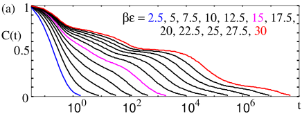
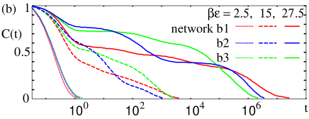
Figure 1: (a)(b) Relaxation time course for four sets of networks ($M=24$, $K=8$) for several $\beta$.

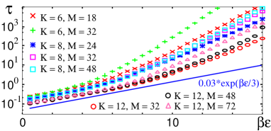
Figure 2: Relaxation time as a function of $\beta$ for the sample reaction networks in Fig. 1(a)(b).

In Fig. 1, we give examples of the relaxation time course for four sets of networks ($M=24$, $K=8$), where we plot the deviation from equilibrium concentration defined by $C(t)=\{\sum_{i}(x_{i}(t)-x_{i}^{eq})(x_{i}(0)-x_{i}^{eq})\}/\{\sum_{i}(x_{i}(0)-x_{i}^{eq})^{2}\}$. We note two salient behaviors when $\beta$ is sufficiently larger than $\beta_{c}\sim 3/\varepsilon$, which is the inverse of the average difference between energy levels. First, there exists overall $\log(t)$ relaxation, in contrast to exponential relaxation for small $\beta$. Second, there are several plateaus in the relaxation course. The logarithmic relaxation at large $\beta$ is generally observed, independently of the networks or K. Existence of plateaus is also universal. The number of plateaus depends on each network (Fig. 1(b)); generally, the number decreases as $K$ increases.

The integrated relaxation time $\tau=<\int_{0}^{\infty}|C(t)|dt>$ is plotted as a function of $\beta$ for several $M$ and $K$ in Fig. 2, where $<\cdots>$ is the average over networks with given $M$ and $K$. For the small $\beta$ regime in which $C(t)$ decays exponentially, $\tau$ follows $\exp(\beta/\beta_{c})$. It is the inverse of the average reaction rate to increase the energy, which gives the order of the relaxation timenote_r . For large $\beta$ giving $\log(t)$ relaxation, $\tau$ follows $\exp(R\beta\varepsilon)$ with $R$ approaching a larger constant with the increase in $\beta$. $R$ increases with the increase (decrease) in $M$ ($K$), respectively.

The $\log(t)$ relaxation with plateaus is often observed in glass theory and experimentsGR1 ; KCM1 . In the present case, these relaxation characteristics are partially explained by a rough estimate of the eigenvalue distribution in linear stability analysis. Consider deviation from the equilibrium concentration as $x_{i}(t)=x^{eq}_{i}+\delta x_{i}(t)$, where the equilibrium concentration $x_{i}^{eq}=s\exp(-\beta E_{i})$ is the fixed point solution of eq. (2). By linearizing with $\delta x_{i}(t)$ ($i=1,\cdots,M$), we get ${\bf\delta\dot{x}(t)}=\bf{J}{\bf\delta x(t)}$ with the Jacobi matrix $\bf{J}$ computed straightforwardly. For large $\beta$, $J_{i,j}$ for $i>j$, given by $Con(i,j;c^{\prime})x_{c^{\prime}}^{eq}e^{-\beta(E_{i}-E_{j})}$, is much smaller than that for $i<j$, $Con(i,j;c")x_{c"}^{eq}$. If the former terms are neglected, the above $\bf{J}$ is a triangular matrix, so that the eigenvalues $\lambda_{i}$ of $\bf{J}$ are given by diagonal elements $J_{i,i}=-\sum_{j<i}Con(i,j;c")x_{c"}^{eq}-\sum_{j>i}Con(i,j;c^{\prime})x_{c^{\prime}}^{eq}e^{\beta(E_{i}-E_{j})}$, whose distribution has similar dependence to that of $\exp(-\beta E_{k})$, for large $\beta$. This is also true for the neglected off-diagonal terms. Hence, it is expected that the distribution of the eigenvalues $\lambda_{i}$ is similar to the distribution of $\exp(-\beta E_{k})$, for large $\beta$ (besides the null eigenvalue $\lambda_{0}=0$ corresponding to the equilibrium distribution). In fact, numerical diagonalization of the Jacobian matrix supports this estimate of eigenvalue distribution. By using this linear approximation and the correspondence of the eigenvalue with $\exp(-\beta E)$, $C(t)$ is approximated by $\int_{0}^{\varepsilon}D(E)a(E)\exp(-e^{-\beta E}t)dE$, with the distribution of energy $D(E)$, which is roughly homogeneous, and the fractions of the eigenmodes $a(E)$ in the initial condition, which are almost equal. Hence, $D(E)$ and $a(E)$ are roughly constantnote3 . By setting $u=\exp(-\beta E)t$, the integral is rewritten as $(1/\beta)\int_{te^{-\beta\varepsilon}}^{t}(1/u)e^{-u}du$. By taking a limit of $\beta\to\infty$ first, $\log(t)$ dependence is obtained asymptotically for large $t$.

Though this estimate is originally asymptotic for large $t$, we used it for the time span where many eigenvalues contribute to the relaxation. For the last stage of the relaxation, only a few eigenvalues contribute. If there is a gap $\Delta\lambda$ between two neighboring eigenvalues, there is a plateau in the relaxation for the time span $\frac{1}{\Delta\lambda}$. For large $\beta$, the gap between eigenvalues increases so that the existence of a plateau is expected. However, plateaus other than the last one, as well as their number during the relaxation, are not directly obtained from this argument. Here we give a heuristic argument for the plateaus.

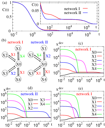
Figure 3: (a) Time course of $C(t)$ for two example networks, I and II, given in (b), with $\beta=16/\varepsilon$. In (b), the chemicals attached to the arrows that display reactions are their catalysts. Time courses of $x^{dev}_{i}(t)$ of (c) network I, and (d) network II corresponding to (a). In (a)(c)(d), all the chemicals are at equal number initially (i.e., $\beta=0$). Time courses of $x^{dev}_{i}(t)$ of network I from the initial condition $x_{i}=1$ for $i=0,2,3$, $x_{1}=0.4$ and $x_{4}=1.6$ are plotted in (e).

In Figs. 3 and 4, we give examples of the relaxation for smaller networks. Besides $C(t)$, we have plotted $x^{dev}_{i}(t)=x_{i}(t)/x^{eq}_{i}$ in Figs. 3(c)-(e) and 4(c). At each plateau, there are cluster(s) of elements in which $x^{dev}_{i}(t)$ takes almost the same value. Within each cluster, chemicals are in local equilibrium through mutual reactions, whereas the equilibration process with elements out of the cluster is suppressed, since the concentrations of the catalytic components responsible for reactions for such equilibration are low. Consider a chemical with $x^{dev}_{i}$ larger than the others. If the concentration of the catalyst(s) necessary to equilibrate the abundant chemical is small, the equilibration process is suppressed. Negative correlation in the abundances between the excess chemical and its catalyst will further suppress the relaxation to equilibrium. We now illustrate how this negative correlation gives rise to plateaus consisting of local-equilibrium clusters, by using examples given in Figs. 3 and 4.

In the networks I and II in Fig. 3(b), consisting of 5 chemicals, the component $X_{0}$ (with lowest $E$) is transformed to all other components. In cases with large $\beta$, because $E_{0}$ is minimum, chemicals $i\geq 1$ flow into $X_{0}$ from the initial condition with $\beta=0$, having $x^{dev}_{i}(0)>1$ for $i\geq 1$ for large $\beta$. For both the networks, the eigenvalues of $\bf{J}$ are $\exp(-\beta E_{1})$, $\exp(-\beta E_{2})$, $\exp(-\beta E_{4})$, and 0 ($E_{i}=\frac{i}{4}\varepsilon$), asymptotically as $\beta$ becomes large. As shown in Fig. 3(a), however, the numbers of plateaus appearing through the relaxation are different between the two networks.

In network I, the first plateau consists of a local-equilibrium cluster $X_{0}$, $X_{2}$, and $X_{4}$, whereas $X_{3}$ joins to the cluster at the second plateau, as shown in Fig. 3(c). The suppression of equilibration of $X_{1}$ is explained as follows: Relaxation (i.e., decrease) of $X_{1}$ ($X_{4}$) is catalyzed by $X_{4}$ ($X_{1}$), respectively. If one of the species $X_{1}$ or $X_{4}$ decreases faster, the relaxation of the other is suppressed. Because $x^{eq}_{1}$ is larger than $x^{eq}_{4}$, $X_{4}$ relaxes faster, so that the relaxation of $X_{1}$ is suppressed. The negative correlation between the abundances of $X_{1}$ and its catalyst hinders the relaxation of $X_{1}$. Since the relaxations of $X_{2}$ and $X_{4}$ are catalyzed by the abundant $X_{1}$, the local-equilibrium $X_{0}$, $X_{2}$, and $X_{4}$ is first achieved and then $X_{3}$ catalyzed by $X_{2}$ (more abundant than $X_{4}$, the catalyst for $X_{1}$) joins to the cluster.

In network II, on the other hand, the relaxation of $X_{1}$ is not suppressed since its catalyst $X_{2}$ relaxes only slowly because its catalyst $X_{4}$ relaxes faster, as it is catalyzed by abundant $X_{1}$. Negative correlation exists, not between $X_{1}$ and its catalyst, but instead between $X_{2}$ and its catalyst $X_{4}$. Thus, the local equilibrium among $X_{0}$, $X_{1}$, $X_{3}$, and $X_{4}$ is realized to produce only one plateau.

As expected from the above argument, the types of plateaus that appear in the relaxation can depend on the initial condition, because the reactions that are suppressed depend on which catalysts are first decreased. See Fig. 3(e), which shows the relaxation process of network I from the initial condition with $x_{4}=4x_{1}$.

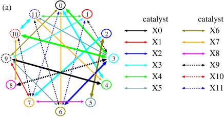
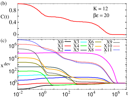
Figure 4: (a) A reaction network with $M=12$ and $K=4$, where the color of each arrow shows the catalyst for the reaction, and thick arrows indicate ”major relaxation” for each chemical (see text). (b) Time course of $C(t)$ for the network, and (c) time courses of $x^{dev}_{i}(t)$ for $\beta=20/\varepsilon$.

For complex catalytic reaction networks, the argument is not so simple, but the existence of local equilibria and suppression of relaxation by the negative correlation mechanism generally underlie the formation of plateaus. Figure 4(a) is a catalytic reaction network with $M=12$ and $K=4$, and Fig. 4(b)(c) show the time courses of $C(t)$ and $x^{dev}_{i}(t)$ for $\beta=20/\varepsilon$. As shown in Fig. 4(b), this network exhibits three plateaus in the relaxation process. At each plateau, chemicals $i=1,\cdots M$ are clustered into a few groups within which $x^{dev}_{i}$ is almost constant (Fig. 4(c)). The following clusters are formed successively: $\{X_{0},X_{4}\}$, $\{X_{3},X_{6}\}$, and $\{X_{10},X_{11}\}$ at the first plateau, $\{X_{0},X_{3},X_{4},X_{6}\}$, $\{X_{5},X_{7}\}$, and $\{X_{10},X_{11}\}$ at the second plateau, and $\{X_{0},X_{1},\cdots,X_{7},X_{9}\}$ and $\{X_{10},X_{11}\}$ at the third plateau.

Each of these plateaus is explained by checking if the catalyst for the “major h relaxation process for each $X_{i}$ is abundant, which is a path catalyzed by $X_{k}$ with the smallest $k$ among the reactions with $j$ smaller than $i$. At the first plateau, $X_{3}$ and $X_{4}$ have negative correlation since the major relaxation of $X_{3}$ is the reaction catalyzed by $X_{4}$, and that of $X_{4}$ by $X_{3}$, so that the formation of the cluster $\{X_{0},X_{4}\}$ suppresses the equilibration between $X_{0}$ and $X_{3}$.

At the second plateau, $\{X_{3},X_{6}\}$ and $\{X_{5},X_{7}\}$ clusters have the following negative correlation. For $\{X_{5},X_{7}\}$ clusters, the reactions $X_{5}+X_{6}\to X_{2}+X_{6}$ and $X_{7}+X_{3}\to X_{2}+X_{3}$ give the major relaxations. On the other hand, the reactions $X_{6}+X_{7}\to X_{0}+X_{7}$ and $X_{3}+X_{4}\to X_{3}+X_{4}$ give the major relaxations for the $\{X_{3},X_{6}\}$ cluster, but the reaction $X_{3}+X_{4}\to X_{3}+X_{4}$ is suppressed since its catalyst $X_{4}$ has already been decreased. In this case, the cluster$\{X_{5},X_{7}\}$ does not join $X_{2}$, whereas the clusters $\{X_{3},X_{6}\}$ and $\{X_{0},X_{4}\}$ aggregate.

In general, among a variety of chemical components, there exists such a negative correlation between chemicals in excess and the catalysts to decrease them towards equilibrium. Then, the equilibration of the chemicals is suppressed, leading to a plateau in the relaxation process.

In this Letter, slow relaxation to equilibrium in catalytic reaction networks is demonstrated. When the temperature of the system is sufficiently lower than $\varepsilon$/3, the average difference between energy levels, overall $\log(t)$ relaxation appears. Several plateaus appear depending on the network and initial condition. The plateaus are not metastable states in the energy landscape but, rather, are a result of kinetic constraints due to a reaction bottleneck, originating in the formation of local-equilibrium clusters and suppression of equilibration by the negative correlation between an excess chemical and its catalyst.

Possible configurations for local-equilibrium clusters are limited, and thus the number and ordering of plateaus are restricted. However, they are not necessarily uniquely determined by the network, but depend on the initial condition, because they are influenced by which catalysts are decreased first. Also, the relaxation is often non-monotonic; the deviation from equilibrium may increase during the relaxation course. Such roundabout relaxation has also been observed in a Hamiltonian system Morita-round . We also note that discreteness in the molecule number results in anomalous reaction dynamics with long time correlationsAK2 , and further suppresses the relaxation in the catalytic reaction networkinprep .

The behaviors reported here are reminiscent of the relaxation in glass. Our model, as studied here, has a kinetic constraint, although the constraint is based on the network structure rather than the spatial configuration. Application of theoretical frameworks developed in the study of glasses will be important to our chemical net glass in future work. Maintenance of the quasi-stationary states reported here, as well as successive changes in them, are often observed in biochemical processes, which have a large variance of reaction rates, i.e., potentiality of $\varepsilon\gg 1/\beta$. In future work, it will be important to discuss the relevance of the present “glassy h dynamics to intracellular reactions.

The authors would like to thank M. Tachikawa, S. Sano, and S. Ishihara for discussions. (A. A.) This research was supported in part by a Grant-in Aid for Young Scientist (B) (Grant No. 19740260).

References

- (1) E. Schrödinger, What is life?, Cambridge Univ. Press (1946)
- (2) G. Nicolos and I. Prigogine: Self-Organization in Nonequlibrium Systems (John Wiley & Sons, 1977).
- (3) F. H. Stillinger and T. A. Weber, Phys. Rev. A 25 978 (1982)
- (4) G. Biroli and J. Kurchan, Phys. Rev. E 64 016101 (2001)
- (5) P. G. De Benedetti and F. H. Stillinger, Nature 401 259 (2001)
- (6) W. Kob, 2003 Slow relaxations and nonequilibrium dynamics in condensed matter (Les Houches 2002 ) eds. Barrat J L et al. (Berlin: Springer) 199
- (7) N. Nakagawa and K. Kaneko, J. Phys. Soc. Jpn. 69 1255 (2000); Phys. Rev. E 64 055205(R)
- (8) H. Morita and K. Kaneko, Europhys. Lett. 66 198 (2003); Phys. Rev. Lett. 96 050602 (2006)
- (9) A. Awazu and K. Kaneko, Phys. Rev. Lett. 92 258302 (2004)
- (10) R.S. Shaw et al., Proc Nat. Acad. Sci. USA, 104 (2007) 9580; A. Awazu, Phys. Rev. E63, 032102 (2001)
- (11) F. Ritort and P. Sollich, Adv. Phys. 52 219 (2003)
- (12) S. Whitelam, L. Berthier and J P. Garrahan, Phys. Rev. E 71 026128 (2005)
- (13) C. Toninelli and G. Biroli, J. Stat. Phys. 126 731 (2007)
- (14) We can adopt other forms of satisfying the detailed balance, say . Overall qualitative behaviors – relaxation and existence of plateaus – are not altered.
- (15) Qualitatively identical behaviors are obtained even for a Gaussian distribution of energy levels, or bounded distributions. For log-normal or power-law distributions of energy, the relaxation behavior is altered.
- (16) By linearizing the relaxation dynamics to equilibrium (as discussed later), and by replacing the energy difference between chemicals by the average , we get under suitable approximation.
- (17) As long as there is no singular dependence of and on (such as the power law dependence) the estimate below is valid.
- (18) H. Morita and K. Kaneko, Phys. Rev. Lett. 94 087203 (2005)
- (19) A. Awazu and K. Kaneko, Phys. Rev. E 76 041915 (2007)
- (20) S. Sano, A. Awazu, K. Kaneko, in preparation.