An approach to construct wave packets with complete classical-quantum correspondence in non-relativistic quantum mechanics
Abstract
We introduce a method to construct wave packets with complete classical and quantum correspondence in one-dimensional non-relativistic quantum mechanics. First, we consider two similar oscillators with equal total energy. In classical domain, we can easily solve this model and obtain the trajectories in the space of variables. This picture in the quantum level is equivalent with a hyperbolic partial differential equation which gives us a freedom for choosing the initial wave function and its initial slope. By taking advantage of this freedom, we propose a method to choose an appropriate initial condition which is independent from the form of the oscillators. We then construct the wave packets for some cases and show that these wave packets closely follow the whole classical trajectories and peak on them. Moreover, we use de-Broglie Bohm interpretation of quantum mechanics to quantify this correspondence and show that the resulting Bohmian trajectories are also in a complete agreement with their classical counterparts.
Keywords: Schrödinger equation; Classical-quantum
correspondence; Wave packets.
1 Introduction
The issue of classical-quantum correspondence has been extensively investigated in the literature [1]. Moreover, the question of construction and interpretation of wave packets in quantum mechanics and its connection with classical mechanics has been attracting much attention. In quantum physics, one is generally concerned with the construction of wave packets by the superposition of the energy eigenstates which would peak around the classical trajectories. These efforts have been started by Schrödinger [2] and followed by others who were interested in finding quantum mechanical states which provide a close connection between classical and quantum formulations of a given physical system in the context of the coherent states [3]. These states can also be generated using algebraic methods [4], supersymmetric quantum mechanics [5] and its application to different physical situations [6].
In this paper, we pursue a different approach to construct wave packets with complete classical and quantum correspondence. First, we consider similar Schrödinger equations of two oscillators with and variables. Classically, we can easily solve this model and find the behavior of the variables versus time (). If these two oscillators have the same total energy, the solutions will be equivalent up to a temporal phase factor. Imposing particular initial conditions, we will obtain the trajectories in the configuration space (). Inversely, using the form of the trajectories, again we can find the temporal behavior of the variables. For instance, in general, the trajectory for the case of a simple harmonic oscillator (SHO) is an ellipse. Therefore, we can obtain the time behavior of the variables as and , where corresponds to a circle. Thus, we can parameterize the behavior of one variable (e.g. ) versus another variable (e.g. ) where they both satisfy the same equation of motion.
Our motivation for this model is related to its interesting quantum mechanical properties. In the quantum version, this model allows us to define a wave function which is a function of and unlike the usual case where the wave function is a function of or and time. As we shall see, the existence of the two mentioned similar oscillators results in a hyperbolic partial differential equation (PDE). Therefore, we are free to choose the initial wave function and the initial slope of the wave function. This freedom for choosing the initial conditions (or the expansion coefficients) allows us to obtain a specific form of the wave packets with complete classical and quantum correspondence. In fact, the initial wave function and its derivative correspond to classical initial position and initial momentum, respectively. To fix the expansion coefficients, we will apply the prescription used in Refs. [7, 8, 9] for the case of hyperbolic PDEs which also appear in the context of quantum cosmology.
The purpose of this paper is to construct wave packets such that the classical and quantum correspondence is manifest, which means that the wave packet should be centered around the classical path and the crest of the wave packet should follow the classical path as closely as possible. Usually, the temporal behavior of the variables is studied in literature where its underlying equation is parabolic. But here, we are encountered with the hyperbolic PDEs which correspond to the classical picture of parametric trajectories. Although both descriptions are equivalent, the latter contains some interesting properties in quantum domain which allows us to obtain the complete classical-quantum correspondence for any oscillator using a unique prescription.
To be more precise, we can also quantify this correspondence using de-Broglie Bohm interpretation of quantum mechanics [10]. This approach gives us the Bohmian trajectories which are guided by the wave function. These trajectories are governed by classical plus quantum potential. Therefore, the coincidence between classical and quantum trajectories accrues in the limit of vanishing quantum potential. In fact, the usage of the appropriate initial conditions results in the suppression of the quantum potential [9].
The paper is organized as follows: In Sec. 2, we present the model of two similar oscillators which results in a hyperbolic PDE at the quantum level. We then construct wave packets by choosing the appropriate expansion coefficients which leads to a good correspondence between classical and quantum solutions. In Sec. 3, we use the casual interpretation of quantum mechanics to quantify this correspondence and obtain the Bohmian trajectories for different cases. In Sec. 4, we state our conclusions.
2 The model
In non-relativistic quantum mechanics we can write the dimensionless time independent Schrödinger equation for variable as
| (1) |
where is the potential term which here is supposed to be an even function of its variable and is the total energy. Also we can rewrite the above equation for another variable
| (2) |
Classically, the above equations show two similar oscillatory motions for and variables with equal total energy and the following equations of motion
| (3) |
By assuming specific classical initial conditions, we can obtain a particular trajectory in the configuration space. Here, we impose the following initial conditions:
| (4) |
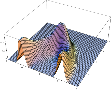
which result in circular motion for the case of simple harmonic oscillators for and variables (Fig. 2). Moreover, the classical behavior of versus time in the presence of some sample potentials is also depicted in the right part of Figs. 3-6 as dashed lines. Note that, the above initial conditions result in classical solutions which have the following property
| (5) |
where is the classical period of motion.
Now, we define a new wave function where and satisfy Eqs. (1) and (2), respectively. Therefore, satisfies the following partial differential equations
| (8) |
Subtracting these equations leads to
| (9) |
where is a hyperbolic differential equation. This equation can be solved using the separation of variables and the general wave packet which satisfies this equation can be written as
| (10) |
Since the potential is an even function of its variable, the eigenfunctions are separated into even and odd categories. Moreover, we have intentionally separated the odd and even terms for further usages. To find the exact form of the wave function we need to specify the expansion coefficients. These coefficients will be determined from the initial form of the wave function which is evaluated along axis () in consistency with the classical initial conditions (4).
Now, let us consider the initial behavior of the wave function. The wave function and the first derivative of the wave function at take the form
| (11) | |||
| (12) |
Therefore, the coefficients determine the initial wave function and the coefficients determine the initial derivative of the wave function. From a mathematical point of view, since the underling differential equation (9) is second order, s and s are arbitrary and independent variables. On the other hand, if we are interested to construct wave packets which simulate the classical behavior with known classical positions and momentums, all of these coefficients will not be independent. It is obvious that the presence of odd terms dose not have any effect on the form of the initial wave function but they are responsible for the slope of the wave function at , and vice versa for the even terms. Now, consider the behavior of the initial wave function. Near the differential equation (9) takes the form
| (13) |
which has the solution as
| (14) |
where and satisfy
| (15) | |||||
| (16) |
and ’s are separation constants. These equations are Schrödinger equations with ’s as their energy levels. Equation (15) is exactly solvable with plane wave solutions
| (17) |
where and are arbitrary complex numbers. We can find the eigenfunctions and the eigenvalues of equation (16) using numerical techniques like Spectral Method [11] with an acceptable accuracy. Now, the general solution to Eq. (13) can be written as
| (18) |
As stated before, this solution is valid only for small . Therefore, we can write the initial conditions as follows
| (19) | |||||
| (20) |
where prime denotes the derivative with respect to . Obviously, a complete description of the problem would include the specification of both of these quantities. However, since we are interested to construct wave packet with classical properties, we need to assume a specific relationship between these coefficients. The prescription is that the coefficients have the same functional form [7, 8, 9] i.e.
| (21) | |||||
| (22) |
where is a function of . In terms of s and s we have
| (23) | |||||
| (24) |
First, let us apply this method to the simplest (bounded) case which is an infinite square well
| (25) |
with well-known orthonormal even and odd eigenfunctions (here stands for or )
| (26) |
Since the energy spectrum for this model is , using the exact form of the eigenstates, we can find the desired expansion coefficients (23)
| (27) | |||||
| (28) |
which result in the following wave packet
| (29) |
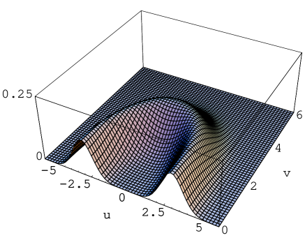
To completely determine the wave packet, we need to specify the functional form of . On the other hand, we can choose by imposing an appropriate initial condition (21) which we choose as two Gaussian peaked at
| (30) |
This choice of initial condition is equal to the following form of the expansion coefficient
| (31) | |||||
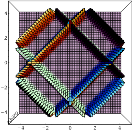
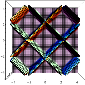
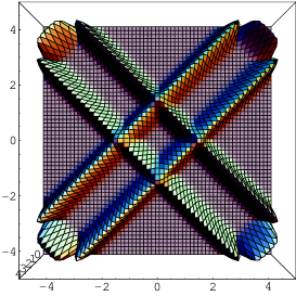
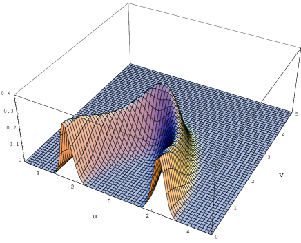
where is the imaginary error function . In Fig. 1, we have shown the resultant wave packets for different values of and . Classically, the particle is free inside the well and can begin its one-dimensional motion with positive or negative initial velocity and from any position between . As it can seen from the figure, the behavior of the wave packets are in complete agreement with the classical scenario and they strongly peak on the classical trajectories. In fact, the value of determines the initial classical position. The presence of two rectangles with opposite direction shows the two possible direction of initial motion at . Since the wave packets follow some straight lines, its classical picture consists of a free particle with constant velocity. Moreover, the height of the crest of the wave packet is constant along the classical trajectories which shows that the probability of finding the particle is constant along the classical path. On the other hand, since the classical velocity of the particle for this case is a constant of motion, the classical probability of finding the particle is also constant along its trajectory. Although this method is generally applicable for one-dimensional systems, we can also obtain a class of two-dimensional classical and quantum correspondences for this especial case. As the figure shows, these wave packets correspond to the cases of equal absolute velocities in and directions () with arbitrary initial position.
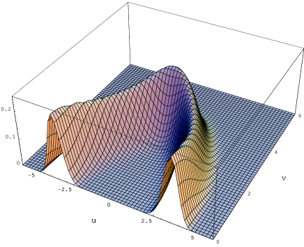
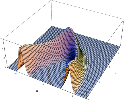
Now, we study other cases with polynomial or exponential form of the potential. First, we should choose an appropriate functional form of . This means that, we need to specify in such a way that the initial wave function has a desired classical description (see Figs. 2-6). We will see that this choice of coefficients leads to complete classical and quantum correspondence in all the studied cases. In the left part of Figs. 2-6, we have depicted the wave packets for some sample potentials. As it can be seen from the figures, the wave packets closely follow the classical paths and peak on them. Before discussing the solutions, we outline the causal interpretation of quantum mechanics and use it to interpret the results in the next section.
3 The causal interpretation
To make the connection between the classical and quantum results more concrete, we use the causal interpretation of quantum mechanics [8, 9, 10]. In this interpretation the wave function can be written as
| (32) |
where and are real functions and satisfy the following equations
| (33) | |||||
| (34) |
To write and , it is more appropriate to separate the real and imaginary parts of the wave function
| (35) |
where are real functions of and . Using equation (32) we have
| (36) | |||||
| (37) |
On the other hand, the Bohmian trajectories are governed by
| (38) | |||
| (39) |
where the momenta correspond to the classical related Lagrangian . Therefore, the Bohmian equations of motion take the form
| (40) | |||
| (41) |
These differential equations can be solved numerically to find the time evolution of and . In the right part of Figs. 2-6, we have shown the Bohmian trajectories as solid lines for five different forms of the potentials
| (47) |
The initial wave functions are chosen to be localized on classical initial positions and also the initial slope is determined by equations (19) and (21). In fact, we are free to choose any arbitrary but appropriate initial wave functions which correspond to the classical scenario. For cases studied here, we choose two different forms of coefficients (Figs. 2-6)
| (48) |
These coefficients are chosen so that the initial wave function contains two bumps along axis which correspond to initial and final classical positions. In fact, these choices are not special and there are many other equivalent alternatives. Since the slope of the wave function is related to the odd terms, the expectation value of the momentum operator is positive and negative respectively for initial and final states of motion in agreement with the classical scenario. Note that, since these two bumps are related to two different physical situations, the integrations are along positive and negative parts of the axis, respectively. Figure 2 shows the resulting wave packet for the simple harmonic oscillator and the Bohmian and classical trajectories. In the right part of figures 3-6, we have also shown the Bohmian and classical behaviors of variable versus time (). The complete correspondence between these results are again manifest. It is worth to mention that for the cases where , we need to choose complex [12]. Beside the stated advantages, this method has also some limitations. As we have shown by various examples, this method works well for symmetric bounded potentials. This class of potentials results in oscillatory classical motions which can be followed by wave packets with a finite set of eigenfunctions. Therefore, this method, in the present fashion, is not applicable even for simple unbounded situations like free particle, potential barrier, delta function potential and etc. The generalization of this method for the case of free particles is the subject of our future work.
4 Conclusions
In this work, we have studied the classical-quantum correspondence in the context of non-relativistic quantum mechanics. First, we considered two similar oscillators for and variables and obtained the classical trajectories. Since these two variables satisfy the same equation of motion, we obtained the trajectory of one variable versus another one by choosing a particular set of initial condition. In the quantum version, this scenario leads to a hyperbolic partial differential equation where its solution contains infinite unknown coefficients. Half number of these coefficients are related to the initial form of the wave function and others correspond to the initial slope of the wave function. Upon using a specific relation between these coefficients and choosing appropriate initial wave functions we can construct desired wave packets. The crests of these wave packets closely follow the classical paths from initial position to the final position. We have quantified this correspondence using de-Broglie Bohm interpretation of quantum mechanics. We applied this method to various cases and showed that the resulting wave packets completely simulate their classical counterpart’s behavior. In particular, the Bohmian trajectories coincided well with classical trajectories for the all cases.
Acknowledgements
I would like to thank M. Mirzaei for his useful comments and discussions.


References
- [1] A. O. Bolivar, Quantum-classical correspondence: dynamical quantization and the classical limit (Springer, New York, 2004).
- [2] E. Schrödinger, Naturwiss. 14, 664 (1926).
- [3] R. J. Glauber, Phys. Rev. Lett. 10, 84 (1963); Phys. Rev. 130, 2529 (1963); 131, 2766 (1963); M. M. Nieto and L. M. Simmons, Phys. Rev. Lett. 41, 207 (1978); Phys. Rev. A 19, 438 (1979); S. Kais and R. D. Levine, Phys. Rev. A 41, 2301 (1990), G. C. Gerry, Phys. Rev. A 31, 2721 (1985), G. C. Gerry, Phys. Rev. A 33, 2207 (1986); A. M. Perelomov, Generalized coherent states and their applications (Berlin, Springer, 1986).
- [4] I. L. Cooper, J. Phys. A: Math. Gen. 25, 1671 (1992).
- [5] T. Fukui and A. Aizawa, Phys. Lett. A 180, 308 (1993); M. G. Benedict and B. Molnar, Phys. Rev. A 60, R1737 (1999).
- [6] M. M. Nieto and L. M. Simmons, Phys. Rev. D 20, 1332 (1979); M. G. A. Crawford and E. R. Vrscay, Phys. Rev. A 57, 106 (1998); A. H. Kinani and M. Daoud, Phys. Lett. A 283, 291 (2001); C. C. Gerry and J. Kiefer, Phys. Rev. A 37, 665 (1988); J. R. Klauder, J. Phys. A: Math. Gen. 29, L293 (1996); P. Majumdar and H. S. Sharatchandra, Phys. Rev. A 56, R3322 (1997); S. A. Pol shin, J. Phys. A: Math. Gen. 33, L357 (2000); A. Chenaghou and H. Fakhri, Mod. Phys. Lett. A 17, 1701 (2002); M. M. Nieto, Mod. Phys. Lett. A 16, 2305 (2001); D. J. Fernandez, V. Hussin, O. Rosas-Ortiz, J. Phys. A: Math. Theor. 40, 6491 (2007).
- [7] S. S. Goushe, H. R. Sepangi, P. Pedram, and M. Mirzaei, Class. Quantum Grav. 24, 4377 (2007), arXiv:gr-qc/0701035.
- [8] P. Pedram, S. Jalalzadeh, Phys. Lett. B, 660, 1 (2008), arXiv:0712.2593.
- [9] P. Pedram, J. Cosmol. Astropart. Phys. 07, 006 (2008), arXiv:0806.1913.
- [10] P. R. Holland, The Quantum Theory of Motion: An Account of the de Broglie-Bohm Interpretation of Quantum Mechanics, Cambridge University Press, Cambridge (1993).
- [11] J. P. Boyd, Chebyshev and Fourier Spectral Methods, Springer-Verlag, BerlinHeidelberg (1989); P. Pedram, M. Mirzaei and S. S. Gousheh, Comput. Phys. Commun. 176, 581 (2007), arXiv:math-ph/0701015; P. Pedram, M. Mirzaei, S. Jalalzadeh, and S. S. Gousheh, Gen. Rel. Grav. 40, 1663 (2008), arXiv: 0711.3833; P. Pedram, S. Jalalzadeh, S. S. Gousheh, Phys. Lett. B 655, (2007) 91, arXiv:0708.4143.
- [12] P. Pedram, Phys. Lett. B, 671, 1 (2009), arXiv:0811.3668.