Group theoretical study of LOCC-detection of
maximally entangled state using hypothesis testing

Abstract

In the asymptotic setting, the optimal test for hypotheses testing of the maximally entangled state is derived under several locality conditions for measurements. The optimal test is obtained in several cases with the asymptotic framework as well as the finite-sample framework. In addition, the experimental scheme for the optimal test is presented.

I Introduction

Recently various quantum information processings are proposed, and many of them require maximally entangled states as resourcesbbcjpw ; bennett-wiesher ; ekert . Hence, it is often desired to generate maximally entangled states experimentally. In particular, it must be based on statistical method to decide whether the state generated experimentally is really the required maximally entangled state.

Now, entanglement witness is often used as its standard method dariano ; guhne ; horodecki3 ; lewenstein ; terhal . It is, however, not necessarily the optimal method from a viewpoint of statistics. On the other hand, in mathematical statistics, the decision problem of the truth of the given hypothesis is called statistical hypothesis testing, and is systematically studied. Hence, it is desired to treat, under the frame of statistical hypotheses testing, the problem deciding whether the given quantum state is the required maximally entangled state. In statistical hypotheses testing, we suppose two hypotheses (null hypothesis and alternative hypothesis) to be tested a priori, and assume that one of both is true. Based on observed data, we decide which hypothesis is true. Most preceding studies about quantum hypotheses testing concerns only the simple hypotheses testing, in which, both of the null and the alternative hypotheses consist of a single quantum state. For example, quantum Neymann Pearson lemma Ho72 ; helstrom and quantum Stein’s lemmahiai-petz ; ogawa-nagaoka ; Nagaoka-converse ; hayashi-hypo , quantum Chernoff boundACMMABV ; NS , and quantum Hoeffding boundOga-Hay ; H-expo ; N-expo treat simple hypotheses.

However, in a practical viewpoint, it is unnatural to specify both hypotheses with one quantum state. Hence, we cannot directly apply quantum Neymann Pearson theorem and quantum Stein’s lemma, and we have to treat composite hypotheses, i.e., the case where both hypotheses consist of plural quantum states. It is also required to restrict our measurements for testing among measurements based on LOCC (local operations and classical communications) because the tested state is maximally entangled state.

Recently, based on quantum statistical inferencehelstrom ; HolP ; selected , Hayashi et al.tsu discussed this testing problem under statistical hypotheses testing with a locality condition. They treated testing problem where the null hypothesis consists only of the required maximally entangled state. Their analysis has been extended to more experimental settingtheory , and its effectivity has been experimentally demonstrated exper . Modifying this setting, Owari and Hayashi OH clarified the difference in performance between the one-way LOCC restriction and the two-way LOCC restriction in a specific case. Especially, Hayashi et al.tsu studied the optimal test and the existence of the uniformly optimal test (whose definition will be presented later) when one or two samples of the state to be tested are given. Their analysis mainly concentrated the two-dimensional case.

In this paper, we treat the null hypothesis consisting of quantum states whose fidelity for the desired maximally entangled state is not greater than $\epsilon$, and discuss this testing problem with several given samples of the tested state in the following three setting concerning the range of our measurements. (Note that our previous paper tsu treats the case of $\epsilon=0$.) In this problem, there are two kinds of locality restrictions. L1: One is locality concerning the two distinct parties. L2: The other is that concerning the samples. M1: All measurements are allowed. M2: There is restriction on the locality L1, but no restriction on the locality L2. M3: There is restriction on the locality L2 as well as L1. The restrction M3 for measurement is discussed by Virmani and Plenio virmani-plenio , the first time. Hayashi et al.tsu treated the settings M2 and M3, more systematically.

This paper mainly treats the case of sufficiently many samples, i.e., the first order asymptotic theory. As a result, we find that there is no difference in performances of both settings M1 and M2. Especially, the test achieving the asymptotically optimal performance can be realized by quantum measurement with quantum correlations between only two local samples. That is, even if we use any higher quantum correlations among local samples, no further improvement is available under the first order asymptotic frame work. In the two-dimensional case, the required measurement with local quantum correlations is the four-valued Bell measurement between the local two samples. In the setting M3, we treat the null hypothesis consisting only of the maximally entangled state. Then, it is proved that even if we use classical correlation between local samples for deciding local measurement, there is no further improvement. That is, the optimal protocol can be realized by repeating the optimal measurement in the one-sample case in the setting M3.

Concerning the non-asymptotic setting, we derive the optimal test with arbitrary finite number of samples under a suitable group symmetry. This result can be trivially extended to hypothesis testing of arbitrary pure state. Moreover, we derive the optimal test with two samples under the several conditions, and calculate its optimal performance.

Furthermore, we treat the case when each sample system consists of two or three different quantum systems whose state is a tensor product state of different states. In this case, even if the number of samples is one, every party consists of multiple systems. As a result, we obtain the optimal test for the one-sample case in both settings M2 and M3. It is proved that repeating the optimal measurement for one sample gives the test achieving the asymptotically optimal performance. Moreover, when each sample system consists of two different system, it is shown that the optimal measurement for the one-sample case can be realized by a four-valued Bell measurement on the respective parties. Repeating this measurement yields the optimal performance in the first order asymptotic framework. (Indeed, it is difficult to perform the quantum measurement with quantum correlation between two samples because we need to prepare two samples from the same source at the same time. However, in this formulation, it is sufficient to prepare two state from the different source.) When each sample system consists of three different systems, the optimal measurement can be described by the GHZ state $\frac{1}{\sqrt{d}}\sum_{i}|i\rangle|i\rangle|i\rangle$, where $d$ is the dimension of the system. This fact seems to indicate the importance of the GHZ state in the three systems.

Concerning locality restriction on our measurement, it is natural to treat two-way LOCC, but we treat one-way LOCC and separable measurement. This is because the separability condition is easier to treat than two-way LOCC. Hence, this paper mainly adopts separability as a useful mathematical condition. It is contrast that Virmani and Plenio virmani-plenio used the PPT condition and Hayashi et al.tsu partially used the PPT condition.

This paper is organized as follows. The mathematical formulation of statistical hypotheses testing is given in section II and, the group theoretical symmetry is explained in section III.2. In section III.3, we explain the restrictions of our measurement for our testing, for example, one-way LOCC, two-way LOCC, separability, etc. In section IV, we review the fundamental knowledge of statistical hypotheses testing for the probability distributions as preliminary. In section V(section VI, section VII), the setting M1(M2, M3) is discussed, respectively. Further results in the two-dimensional case are presented in section VIII. Finally, in section IX (section X), we discuss the case of two (three) different quantum states, respectively.

II Mathematical formulation of quantum hypothesis testing

Let ${{\cal H}}$ be a finite-dimensional Hilbert space corresponding to the physical system of interest. Then, the state is described by a density matrix on ${{\cal H}}$. In the quantum hypothesis testing, we assume that the current state $\rho$ of the system is unknown, but is known to belong to a subset ${{\cal S}}_{0}$ or ${{\cal S}}_{1}$ of the set of densities. Hence, our task is testing

$$H_{0}:\rho\in{{\cal S}}_{0}\quad\mbox{versus}\quad H_{1}:\rho\in{{\cal S}}_{1}$$ (1)

based on an appropriate measurement on ${{\cal H}}$. That is, we are required to decide which hypothesis is true. We call $H_{0}$ a null hypothesis, and we call $H_{1}$ an alternative hypothesis.

A test for the hypothesis (1) is given by a Positive Operator Valued Measure (POVM) $\{T_{0},T_{1}\}$ on ${{\cal H}}$ composed of two elements, where $T_{0}+T_{1}=I$. For simplicity, the test $\{T_{0},T_{1}\}$ is described by the operator $T=T_{0}$. Our decision should be done based on this test as follows: We accept $H_{0}$ (=we reject $H_{1}$) if we observe $T_{0}$, and we accept $H_{1}$ (=we reject $H_{0}$) if we observe $T_{1}$. In order to treat its performance, we focus on the following two kinds of errors.: A type 1 error is an event such that we accept $H_{1}$ though $H_{0}$ is true. A type 2 error is an event such that we accept $H_{0}$ though $H_{1}$ is true. Hence, we treat the following two kinds of error probabilities: The type 1 error probability $\alpha(T,\rho)$ and the type 2 error probabilities $\beta(T,\rho)$ are given by

$$\alpha(T,\rho) =\mathop{\rm Tr}\nolimits(\rho T_{1})=1-\mathop{\rm Tr}\nolimits(\rho T)\ (\rho\in{{\cal S}}_{0}),$$

$$\beta(T,\rho) =\mathop{\rm Tr}\nolimits(\rho T_{0})=\mathop{\rm Tr}\nolimits(\rho T)\ (\rho\in{{\cal S}}_{1}).$$

A quantity $1-\beta(T,\rho)$ is called power. A test $T$ is said to be level-$\alpha$ if $\alpha(T,\rho)\leq\alpha$ for any $\rho\in{{\cal S}}_{0}$.

In hypothesis testing, we restrict our test to tests whose first error probability is greater than a given constant $\alpha$ for any element $\rho\in{{\cal S}}_{0}$. That is, since the type 1 error is considered to be more serious than the type 2 error in hypothesis testing, it is required to guarantee that the type 1 error probability is less than a constant which is called level of significance or level. Hence, a test $T$ is said to be level-$\alpha$ if $\alpha(T,\rho)\leq\alpha$ for any $\rho\in{{\cal S}}_{0}$.

Then, under this condition, the performance of the test is given by $1-\beta(T,\rho)$ for $\rho\in{{\cal S}}_{1}$, which is called power. Therefore, we often optimize the type 2 error probability as follows:

$$\beta_{\alpha}({\cal S}_{0}\|\rho) \stackrel{{\scriptstyle\rm def}}{{=}}\min_{T\in{{\cal T}}_{\alpha,{\cal S}_{0}}}\beta(T,\rho),$$

$${\cal T}_{\alpha,{\cal S}_{0}} \stackrel{{\scriptstyle\rm def}}{{=}}\{T|0\leq T\leq I,\quad\alpha(T,\rho)\leq\alpha\forall\rho\in{{\cal S}}_{0}\}$$

for any $\rho\in{{\cal S}}_{1}$. Especially, a test $T\in{{\cal T}}_{\alpha,{\cal S}_{0}}$ is called a Most Powerful (MP) test with level $\alpha$ at $\rho\in{{\cal S}}_{1}$ if $\beta(T,\rho)\leq\beta(T^{\prime},\rho)$ for any level-$\alpha$ test $T^{\prime}\in{{\cal T}}_{\alpha,{\cal S}_{0}}$, that is,

$$\beta(T,\rho)=\beta_{\alpha}({\cal S}_{0}\|\rho).$$

Moreover, a test $T\in{{\cal T}}_{\alpha,{\cal S}_{0}}$ is called a Uniformly Most Powerful (UMP) test if $T$ is MP for any level-$\alpha$ test $\rho\in{{\cal S}}_{1}$, that is,

$$\beta(T,\rho)=\beta_{\alpha}({\cal S}_{0}\|\rho),\quad\forall\rho\in{{\cal S}}_{1}.$$

However, in certain instances, it is natural to restrict our testings to those satisfying one or two conditions ($C_{1}$ or $C_{1}$ and $C_{2}$). In such a case, we focus on the following quantity in stead of $\beta(T,\rho)$:

$$\beta_{\alpha,C_{1}}^{C_{2}}(S_{0}\|\rho) \stackrel{{\scriptstyle\rm def}}{{=}}\min_{T\in{{\cal T}}_{\alpha,S_{0}}}\{\beta(T,\rho)|\hbox{$T$ satisfies $C_{1}$ and $C_{2}$.}\}.$$

If a test $T\in{{\cal T}}_{\alpha,S_{0}}$ satisfies conditions $C_{1}$, $C_{2}$, and

$$\beta(T,\rho)=\beta_{\alpha,C_{1}}^{C_{2}}({\cal S}_{0}\|\rho),\quad\forall\rho\in{{\cal S}}_{1},$$

it is called a Uniformly Most Powerful $C_{1},C_{2}$ (UMP $C_{1},C_{2}$) test.

be $T$.

III Our formulations

III.1 Hypothesis

Our target is teasting wheather the generated state is sufficiently close to the maximal entangled state

$$|\phi^{0}_{AB}\rangle=\frac{1}{\sqrt{d}}\sum_{i=0}^{d-1}|i\rangle_{A}\otimes|i\rangle_{B}$$

on the tensor product space ${\cal H}_{A,B}$ of the two $d$-dimensional systems ${\cal H}_{A}$ and ${\cal H}_{B}$ spanned by $|0\rangle_{A},|1\rangle_{A},...,|d-1\rangle_{A}$ and $|0\rangle_{B},|1\rangle_{B},...,|d-1\rangle_{B}$, respectively. Note that we refer to $\{|i\rangle_{A}\}$ and $\{|i\rangle_{B}\}$ as the standard basis. Suppose that $n$ independent samples are provided, that is, the state is given in the form

$$\rho=\bigotimes_{i=1}^{n}\sigma_{i}=\underbrace{\sigma_{1}\otimes\cdots\otimes\sigma_{n}}_{n}$$

for $n$ unknown densities $\sigma_{1},\ldots\sigma_{n}$. We also assume that these densities $\sigma_{1},\ldots,\sigma_{n}$ equal a density $\sigma$. In this case, the state $\rho$ is called $n$-independent and identical density ($n$-i.i.d.). In the following, we consider two settings for our hypotheses:

$$H_{0}: \quad\sigma\in{\cal S}_{\leq\epsilon}\stackrel{{\scriptstyle\rm def}}{{=}}\{\sigma|1-\langle\phi^{0}_{AB}|\sigma|\phi^{0}_{AB}\rangle\leq\epsilon\}$$

versus

$$H_{1}: \quad\sigma\in{\cal S}_{\leq\epsilon}^{c}$$

and

$$H_{0}: \quad\sigma\in{\cal S}_{\geq\epsilon}\stackrel{{\scriptstyle\rm def}}{{=}}\{\sigma|1-\langle\phi^{0}_{AB}|\sigma|\phi^{0}_{AB}\rangle\geq\epsilon\}$$

versus

$$H_{1}: \quad\sigma\in{\cal S}_{\geq\epsilon}^{c}.$$

When the null hypothesis is “$\sigma\in{\cal S}_{\leq\epsilon}$”, the set of level $\alpha$-tests is given in the $n$-fold i.i.d. case by

$${\cal T}_{\alpha,\leq\epsilon}^{n}\stackrel{{\scriptstyle\rm def}}{{=}}\left\{T\left|0\leq T\leq I,\quad\forall\sigma\in{\cal S}_{\leq\epsilon},~{}1-\mathop{\rm Tr}\nolimits\sigma^{\otimes n}T\leq\alpha\right.\right\}.$$

Similarly, when the null hypothesis is “$\sigma\in{\cal S}_{\geq\epsilon}$”, the set of level $\alpha$-tests is given in the $n$-fold i.i.d. case by

$${\cal T}_{\alpha,\geq\epsilon}^{n}\stackrel{{\scriptstyle\rm def}}{{=}}\left\{T\left|0\leq T\leq I,\quad\forall\sigma\in{\cal S}_{\geq\epsilon},~{}1-\mathop{\rm Tr}\nolimits\sigma^{\otimes n}T\leq\alpha\right.\right\}.$$

In this paper, we only treat the null hypothesis ${\cal S}_{\leq\epsilon}$. However, a large part of obtained results can be trivially extended to the case of the null hypothesis ${\cal S}_{\geq\epsilon}$.

III.2 Restriction I: group action

In this paper, we treat these two cases with the invariance conditions for the following group action, which preserve the two hypotheses $H_{0}$ and $H_{1}$. The naturalness of this condition will be discussed later.

1)$U(1)$-action:

$$\phi \mapsto U_{\theta}\phi,\quad\phi\in{\cal H}_{A,B},\quad\theta\in\mathbb{R}$$

where $U_{\theta}$ is defined by

$$U_{\theta} \stackrel{{\scriptstyle\rm def}}{{=}}e^{i\theta}|\phi^{0}_{AB}\rangle\langle\phi^{0}_{AB}|+(I-|\phi^{0}_{AB}\rangle\langle\phi^{0}_{AB}|).$$

For a vector $|u\rangle$ orthogonal to $\langle\phi^{0}_{AB}|$ and a positive number $0\,<p\,<1$, the entanglement properties of the two sates $\sqrt{p}|\phi^{0}_{AB}\rangle+\sqrt{1-p}|u\rangle$ and $e^{i\theta}\sqrt{p}|\phi^{0}_{AB}\rangle+\sqrt{1-p}|u\rangle$ are essentially equivalent. Hence, this symmetry is very natural. We can easily check that this action preserves our hypotheses. The $U(1)$-action is so small that it is not suitable to adopt this invariance as our restriction. However, this invariance can be, often, treated so easily that it be adopted only by a technical reason.

2)$SU(d)$-action: We consider the unitary action on the tensor product space ${\cal H}_{A,B}={\cal H}_{A}\otimes{\cal H}_{B}$:

$$\phi\mapsto U(g)\phi,\quad\phi\in{\cal H}_{A,B},\quad g\in SU(d),$$

where

$$U(g)\stackrel{{\scriptstyle\rm def}}{{=}}g\otimes\overline{g},$$

and $\overline{g}$ is the complex conjugate of $g$ concerning the standard basis $|0\rangle_{B},|1\rangle_{B},...,|d-1\rangle_{B}$ on the system $B$. Indeed, this action preserves the maximally entangled state $|\phi^{0}_{AB}\rangle$. Hence, this action preserves our hypotheses. Furthermore, this action preserves the entanglement property. Similarly to the $U(1)$-invariance, the $SU(1)$-action is so small that it will be adopted only by a technical reason.

3)$SU(d)\times U(1)$-action: Since the $SU(d)$ action and the $U(1)$-action preserve the entanglement property, the following action of the direct sum product group $SU(d)\times U(1)$ of $SU(d)$ and $U(1)$ also preserves this property:

$$\phi\mapsto U(g,\theta)\phi\quad\phi\in{\cal H}_{A,B},\quad(g,e^{i\theta})\in SU(d)\times U(1),$$

where

$$U(g,\theta)\stackrel{{\scriptstyle\rm def}}{{=}}U(g)U_{\theta}=U_{\theta}U(g).$$

Thus, this condition is most suitable as our restriction.

4)$U(d^{2}-1)$-action: As a stronger invariance, we can consider the invariance of the $U(d^{2}-1)$-action, i.e., the following unitary action on the orthogonal space of $|\phi^{0}_{AB}\rangle\langle\phi^{0}_{AB}|$, which is a $d^{2}-1$-dimensional space.

$$\phi\mapsto V(g)\phi,\quad\phi\in{\cal H}_{A,B},\quad g\in U(d^{2}-1).$$

where

$$V(g)\stackrel{{\scriptstyle\rm def}}{{=}}g(I-|\phi^{0}_{AB}\rangle\langle\phi^{0}_{AB}|)+|\phi^{0}_{AB}\rangle\langle\phi^{0}_{AB}|.$$

This group action contains the $U(1)$-action and the $SU(d)$-action. Hence, the invariance of the $U(d^{2}-1)$-action is stronger than the invariances of above three actions. This action does not preserve the entanglement property. Thus, based on this definition, we cannot say that this condition is natural for our setting while it is natural if we are not care of entanglement.

Furthermore, in the $n$-fold i.i.d. setting, it is suitable to assume the invariance of the $n$-tensor product action of the above actions, i.e., $U_{\theta}^{\otimes n}$, $U(g)^{\otimes n}$, $U(g,\theta)^{\otimes n}$, $V(g)^{\otimes n}$, etc.

III.3 Restriction II: locality

When the system consists of two distinct parties $A$ and $B$, it is natural to restrict our testing to LOCC measurements between $A$ and $B$. Hence, we can consider several restrictions concerning locality condition. Hence, in section IV, as the first step, in order to discuss the hypotheses testing with the null hypothesis ${\cal S}_{\leq\epsilon}$, we will treat the following optimization:

$$\beta_{\alpha,G}^{n}(\leq\epsilon\|\sigma)\stackrel{{\scriptstyle\rm def}}{{=}}\min_{T\in{\cal T}_{\alpha,\leq\epsilon}^{n}}\left\{\beta(T,\sigma^{\otimes n})\left|T\hbox{ is $G$-invariant.}\right.\right\},$$

where $G=U(1),SU(d),SU(d)\times U(1),$ or $U(d^{2}-1)$. However, since our quantum system consists of two distant system, we cannot neccessarily use all measurements. Hence, it is natural to restrict our test to a class of tests. In this paper, we focus on the following seven classes.

$\emptyset$:

No condition

$S(A,B)$:

The test is separable between two systems ${\cal H}_{A}^{\otimes n}$ and ${\cal H}_{B}^{\otimes n}$, i.e., the test $T$ has the following form:

$$T=\sum_{i}a_{i}T_{i}^{A}\otimes T_{i}^{B},$$

where $a_{i}\geq 0$ and the matrix $T_{i}^{A}$ ($T_{i}^{B}$) is a positive semi-definite matrix on the system ${\cal H}_{A}^{\otimes n}$ (${\cal H}_{B}^{\otimes n}$), respectively.

$L(A\leftrightarrows B)$:

The test can be realized by two-way LOCC between two systems ${\cal H}_{A}^{\otimes n}$ and ${\cal H}_{B}^{\otimes n}$.

$L(A\to B)$:

The test can be realized by one-way LOCC from the system ${\cal H}_{A}^{\otimes n}$ to the system ${\cal H}_{B}^{\otimes n}$.

$S(A_{1},\ldots,A_{n},B_{1},\ldots,B_{n})$:

The test is separable among $2n$ systems ${\cal H}_{A_{1}}$, …, ${\cal H}_{A_{n}}$, ${\cal H}_{B_{1}}$, …, ${\cal H}_{B_{n}}$, i.e., the test $T$ has the following form:

$$T=\sum_{i}a_{i}T_{i}^{A_{1}}\otimes\cdots\otimes T_{i}^{A_{n}}\otimes T_{i}^{B_{1}}\otimes\cdots\otimes T_{i}^{B_{n}},$$

where $a_{i}\geq 0$ and the matrix $T_{i}^{A_{k}}$ ($T_{i}^{B_{k}}$) is a positive semi-definite matrix on the system ${\cal H}_{A_{k}}$ (${\cal H}_{B_{k}}$), respectively.

$L(A_{1},\ldots,A_{n},B_{1},\ldots,B_{n})$:

The test can be realized by two-way LOCC among $2n$ systems ${\cal H}_{A_{1}}$, …, ${\cal H}_{A_{n}}$, ${\cal H}_{B_{1}}$, …, ${\cal H}_{B_{n}}$.

$L(A_{1},\ldots,A_{n}\to B_{1},\ldots,B_{n})$:

The test can be realized by LOCC among $2n$ systems ${\cal H}_{A_{1}}$, …, ${\cal H}_{A_{n}}$, ${\cal H}_{B_{1}}$, …, ${\cal H}_{B_{n}}$. Moreover, the classical communication among two groups ${\cal H}_{A_{1}}$, …, ${\cal H}_{A_{n}}$ and ${\cal H}_{B_{1}}$,…, ${\cal H}_{B_{n}}$ is restricted to one-way from the former to the later.

Based on the above conditions, we define the following quantity as the optimal second error probability:

$$\beta_{\alpha,n,G}^{C}(\leq\epsilon\|\sigma)\stackrel{{\scriptstyle\rm def}}{{=}} \min_{T\in{\cal T}_{\alpha,\leq\epsilon}^{n}}\left\{\!\beta(T,\sigma^{\otimes n})\left|\begin{array}[]{l}T\hbox{ is $G$-invariant,}\\ \hbox{and satisfies }C\\ \end{array}\!\!\!\right.\right\}.$$

As is easily checked, any LOCC operation is separable. Hence, the condition $L(A\leftrightarrows B)$ is stronger than the condition $S(A,B)$. Also, the condition $L(A_{1},\ldots,A_{n}\to B_{1},\ldots,B_{n})$ is stronger than the condition $S(A_{1},\ldots,A_{n}\to B_{1},\ldots,B_{n})$. The relation among these conditions can be illustrated as follows.

Next, we focus on the trivial relations of the optimal second error probability. If a group $G_{1}$ is greater than $G_{2}$, the inequality

$$\beta_{\alpha,n,G_{1}}^{C}(\leq\epsilon\|\sigma)\geq\beta_{\alpha,n,G_{2}}^{C}(\leq\epsilon\|\sigma)$$ (2)

holds. Moreover, if a condition $C_{1}$ is stronger than another condition $C_{2}$, the similar inequality

$$\beta_{\alpha,n,G}^{C_{1}}(\leq\epsilon\|\sigma)\geq\beta_{\alpha,n,G}^{C_{2}}(\leq\epsilon\|\sigma)$$ (3)

holds.

Similarly, we define $\beta_{\alpha,n,G}^{C}(\geq\epsilon\|\sigma)$ by replacing $\leq\epsilon$ by $\geq\epsilon$ in RHS.

Indeed, if the condition is invariant for the action of $G$, it is very natural to restrict our test among $G$-invariant tests, as is indicated by the following lemma.

Lemma 1

Assume that a set of test satisfying the condition $C$ is invariant for the action of $G$, Then

$$\beta_{\alpha,n,G}^{C}(\leq\epsilon\|\sigma) =\min_{T\in{\cal T}_{\alpha,\leq\epsilon}^{n}}\max_{g\in G}\beta(T,(f(g)\sigma f(g)^{\dagger})^{\otimes n})$$

$$=\min_{T\in{\cal T}_{\alpha,\leq\epsilon}^{n}}\int_{G}\beta(T,(f(g)\sigma f(g)^{\dagger})^{\otimes n})\nu_{G}(dg),$$

where $\nu_{G}$ is the invariant measure and $f$ denotes the action of $G$.

In the following, we sometimes abbreviate the invariant measure $\nu_{G}$ by $\nu$. For a proof see Appendix A. This lemma is a special version of quantum Hunt-Stein lemma HolP . The condition $\emptyset$ is invariant for the actions $U(1),SU(d),SU(d)\times U(1),U(d^{2}-1)$. But, other conditions $S(A,B),L(A\leftrightarrows B)$, $L(A\to B),S(A_{1},\ldots,A_{n},B_{1},\ldots B_{n})$, $L(A_{1},\ldots,A_{n},B_{1},\ldots B_{n})$, $L(A_{1},\ldots,A_{n}\to B_{1},\ldots B_{n})$ are invariant only for $SU(d)$. Hence, Lemma 1 cannot be applied to the pair of these conditions and the actions $U(1),SU(d),SU(d)\times U(1),U(d^{2}-1)$. The following lemma is useful in such a case.

Lemma 2

Assume that the group $G_{1}$ includes another group $G_{2}$ which satisfies the condition of Lemma 1. If

$$\beta_{\alpha,n,G_{1}}^{C}(\leq\epsilon\|\sigma)=\beta_{\alpha,n,G_{2}}^{C}(\leq\epsilon\|\sigma),\quad\forall\sigma$$

then

$$\beta_{\alpha,n,G_{1}}^{C}(\leq\epsilon\|\sigma)$$

$$= \min_{T\in{\cal T}_{\alpha,\leq\epsilon}^{n}}\max_{g\in G_{1}}\beta(T,(f(g)\sigma f(g)^{\dagger})^{\otimes n})$$

$$= \min_{T\in{\cal T}_{\alpha,\leq\epsilon}^{n}}\int_{G_{1}}\beta(T,(f(g)\sigma f(g)^{\dagger})^{\otimes n})\nu_{G_{1}}(dg).$$

Its proof is given in Appendix A.

IV Testing for binomial distributions

In this paper, we use several knowledges about testing for binomial distributions for testing for a maximally entangled state. Hence, we review them here.

IV.1 One-sample setting:

As a preliminary, we treat testing for the coin flipping probability $p$ with a single trial. That is, we assume that the event $1$ happens with the probability $p$ and the event $0$ happens with the probability $1-p$, and focus on the null hypothesis $p\in[0,\epsilon]$. In this case, our test can be described by a map $\tilde{T}$ from $\{0,1\}$ to $[0,1]$, which means that when the data $k$ is observed, we accept the null hypothesis with the probability $\tilde{T}(k)$. Then, the minimum second error probability among level-$\alpha$ tests is given by

$$\beta^{1}_{\alpha}(\leq\epsilon\|q) \stackrel{{\scriptstyle\rm def}}{{=}}\min_{\tilde{T}}\left\{q(\tilde{T})\left|\forall p\in[0,\epsilon],p(\tilde{T})\geq 1-\alpha\right.\right\}$$

$$p(\tilde{T}) \stackrel{{\scriptstyle\rm def}}{{=}}(1-p)\tilde{T}(0)+p\tilde{T}(1).$$

When we define the test $\tilde{T}_{\epsilon,\alpha}^{1}$ by

$$\tilde{T}_{\epsilon,\alpha}^{1}(0)=\left\{\begin{array}[]{ll}\frac{1-\alpha}{1-\epsilon}&\hbox{ if }\epsilon\leq\alpha\\ 1&\hbox{ if }\epsilon\,>\alpha\end{array}\right.,~{}\tilde{T}_{\epsilon,\alpha}^{1}(1)=\left\{\begin{array}[]{ll}0&\hbox{ if }\epsilon\leq\alpha\\ \frac{\epsilon-\alpha}{\epsilon}&\hbox{ if }\epsilon\,>\alpha,\end{array}\right.$$

the test $\tilde{T}_{\epsilon,\alpha}^{1}$ satisfies

$$(1-\epsilon)\tilde{T}_{\epsilon,\alpha}^{1}(0)+\epsilon\tilde{T}_{\epsilon,\alpha}^{1}(1)=1-\alpha.$$ (4)

Moreover, if $p\leq\epsilon$,

$$(1-p)\tilde{T}_{\epsilon,\alpha}^{1}(0)+p\tilde{T}_{\epsilon,\alpha}^{1}(1)\geq 1-\alpha.$$

Hence the test $\tilde{T}_{\epsilon,\alpha}^{1}$ is level-$\alpha$. Furthermore, we can easily check that the minimum of $q(\tilde{T})$ with the condition (4) for $\tilde{T}$ can be attained by $\tilde{T}=\tilde{T}_{\epsilon,\alpha}^{1}$ if $q\,>\epsilon$. Hence,

$$\beta^{1}_{\alpha}(\leq\epsilon\|q)=q(\tilde{T}_{\epsilon,\alpha}^{1})=\left\{\begin{array}[]{ll}\frac{(1-\alpha)(1-q)}{1-\epsilon}&\hbox{ if }\epsilon\leq\alpha\\ 1-\frac{\alpha q}{\epsilon}&\hbox{ if }\epsilon\,>\alpha.\end{array}\right.$$ (7)

IV.2 $n$-sample setting:

In the $n$-trial case, the data $k=0,1,\ldots,n$ obeys the distribution $P^{n}_{p}(k)\stackrel{{\scriptstyle\rm def}}{{=}}\genfrac{(}{)}{0.0pt}{}{n}{k}(1-p)^{n-k}p^{k}$ with the unknown parameter $p$. Hence, we discuss the hypothesis testing with the null hypothesis ${\cal P}_{\leq\epsilon}^{n}\stackrel{{\scriptstyle\rm def}}{{=}}\{P^{n}_{p}(k)|p\leq\epsilon\}$ and the alternative hypothesis $({\cal P}_{\leq\epsilon}^{n})^{c}$. In this case, our test $\tilde{T}$ can be described by a function from the data set $\{0,1,\ldots,n\}$ to interval $[0,1]$. In this case, when the data $k$ is observed, we accept the null hypothesis ${\cal P}_{\leq\epsilon}^{n}$ with the probability $T(k)$. Then, the minimum second error probability among level-$\alpha$ tests is given by

$$\beta^{n}_{\alpha}(\leq\epsilon\|q) \stackrel{{\scriptstyle\rm def}}{{=}}\min_{\tilde{T}}\left\{P^{n}_{q}(\tilde{T})\left|\forall p\in[0,\epsilon],1-P^{n}_{p}(\tilde{T})\leq\alpha\right.\right\}$$

$$P^{n}_{p}(\tilde{T}) \stackrel{{\scriptstyle\rm def}}{{=}}\sum_{k=0}^{n}P^{n}_{p}(k)\tilde{T}(k).$$

We define the test $\tilde{T}^{n}_{\epsilon,\alpha}$ as follows.

$$\tilde{T}^{n}_{\epsilon,\alpha}(k)=\left\{\begin{array}[]{ll}1&k\,<l^{n}_{\epsilon,\alpha}\\ \gamma^{n}_{\epsilon,\alpha}&k=l^{n}_{\epsilon,\alpha}\\ 0&k\,>l^{n}_{\epsilon,\alpha},\end{array}\right.$$

where the integer $l_{\epsilon,\alpha}^{n}$ and the real number $\gamma_{\epsilon,\alpha}^{n}\,>0$, are defined by

$$\sum_{k=0}^{l_{\epsilon,\alpha}^{n}-1}P^{n}_{\epsilon}(k) \,<1-\alpha\leq\sum_{k=0}^{l_{\epsilon,\alpha}^{n}}P^{n}_{\epsilon}(k)$$

$$\gamma_{\epsilon,\alpha}^{n}P^{n}_{\epsilon}(l_{\epsilon,\alpha}^{n}) =1-\alpha-\sum_{k=0}^{l_{\epsilon,\alpha}^{n}-1}P^{n}_{\epsilon}(k).$$

Theorem 1

The test $\tilde{T}^{n}_{\epsilon,\alpha}$ is level-$\alpha$ UMP test with the null hypothesis ${\cal P}_{\leq\epsilon}^{n}$. Hence,

$$\beta^{n}_{\alpha}(\leq\epsilon\|q)=P_{q}^{n}(\tilde{T}_{\epsilon,\alpha})=\sum_{k=0}^{l_{\epsilon,\alpha}^{n}-1}P^{n}_{q}(k)+\gamma_{\epsilon,\alpha}^{n}P^{n}_{q}(l_{\epsilon,\alpha}^{n}).$$

For a proof, see Appendix C.

IV.3 Asymptotic setting

In asymptotic theory, There are two settings at least. One is the large deviation setting, in which the parameter is fixed, hence we focus on the exponential component of the error probability. The other is the small deviation setting, in which the parameter is close to a given fixed point in proportion to the number of samples such that the error probability converges to a fixed number. That is, the parameter is fixed in the former, while the error probability is fixed in the later.

IV.3.1 Small deviation theory

It is useful to treat the neiborhood around $p=0$ as the small deviation theory of this problem for the asymptotic discussion of testing for an maximally entangled state. Hence, we focus on the case that $p=\frac{t}{n}$: Since the probability $P_{t/n}^{n}(k)=\genfrac{(}{)}{0.0pt}{}{n}{k}(1-\frac{t}{n})^{n-k}\left(\frac{t}{n}\right)^{k}$ convergences to the Poisson distribution $P_{t}(k)\stackrel{{\scriptstyle\rm def}}{{=}}e^{-t}\frac{t^{k}}{k!}$. Hence, our testing problem with the null hypothesis ${\cal P}_{\frac{\delta}{n}}$ and the alternative hypothesis $\frac{t^{\prime}}{n}$. is asymptotically equivalent with the testing of Poisson distribution $P_{t}(k)$ with the null hypothesis $t\in[0,\delta]$ and the alternative hypothesis $t^{\prime}$. That is, by defining

$$\beta_{\alpha}(\leq\delta\|t^{\prime}) \stackrel{{\scriptstyle\rm def}}{{=}}\min_{\tilde{T}}\left\{P_{t^{\prime}}(\tilde{T})\left|\forall t\in[0,\delta],1-P_{t}(\tilde{T})\leq\alpha\right.\right\}$$

$$P_{t}(\tilde{T}) \stackrel{{\scriptstyle\rm def}}{{=}}\sum_{k=0}^{\infty}P_{t}(k)\tilde{T}(k),$$

the following theorem holds.

Theorem 2

$$\lim\beta^{n}_{\alpha}\left(\leq\frac{\delta}{n}\left\|\frac{t^{\prime}}{n}\right.\right)=\beta_{\alpha}(\leq\delta\|t^{\prime}).$$

Its proof is given in Appendix D. Similarly to the test $\tilde{T}_{\epsilon,\alpha}^{n}$, we define the test $\tilde{T}_{\delta,\alpha}$ as

$$\tilde{T}_{\delta,\alpha}(k)=\left\{\begin{array}[]{ll}1&k\,<l_{\delta,\alpha}\\ \gamma_{\delta,\alpha}&k=l_{\delta,\alpha}\\ 0&k\,>l_{\delta,\alpha},\end{array}\right.$$

where the integer $l_{\delta,\alpha}$ and the real number $\gamma_{\delta,\alpha}\,>0$, are defined by

$$\sum_{k=0}^{l_{\delta,\alpha}-1}P_{\delta}(k)\,<1-\alpha\leq\sum_{k=0}^{l_{\delta,\alpha}}P_{\delta}(k)$$

$$\gamma_{\delta,\alpha}P_{\delta}(l_{\delta,\alpha})=1-\alpha-\sum_{k=0}^{l_{\delta,\alpha}^{n}-1}P_{\delta}(k).$$

Similarly to Theorem 1, the following theorem holds.

Theorem 3

The test $\tilde{T}_{\delta,\alpha}$ is level-$\alpha$ UMP test with the null hypothesis ${\cal P}_{\leq\delta}\stackrel{{\scriptstyle\rm def}}{{=}}\{P_{t}|t\leq\delta\}$. Hence,

$$\beta^{n}_{\alpha}(\leq\delta\|t^{\prime})=\sum_{k=0}^{l_{\delta,\alpha}-1}P_{t^{\prime}}(k)+\gamma_{\delta,\alpha}P_{t^{\prime}}(l_{\delta,\alpha}).$$

IV.3.2 Large deviation theory

Next, we proceed to the large deviation theory. Using the knowledge of mathematical statistics, we can calculate the exponents of the 2nd error probabilities $\beta^{n}_{\alpha}(\epsilon\|p)$ and $\beta^{n}_{\alpha}(\epsilon\|p)^{\prime}$ for any $\alpha\,>0$ as

$$\lim\frac{-1}{n}\log\beta^{n}_{\alpha}(\leq\epsilon\|p) =d(\epsilon\|p),\hbox{ if }\epsilon\,<p$$

$$\lim\frac{-1}{n}\log\beta^{n}_{\alpha}(\geq\epsilon\|p) =d(\epsilon\|p),\hbox{ if }\epsilon\,>p,$$

where the binary relative entropy $d(\epsilon\|p)$ is defined as

$$d(\epsilon\|p)\stackrel{{\scriptstyle\rm def}}{{=}}\epsilon\log\frac{\epsilon}{p}+(1-\epsilon)\log\frac{1-\epsilon}{1-p}.$$

In the case of $\alpha=0$, we have

$$\frac{-1}{n}\log\beta^{n}_{0}(\epsilon\|p)=\left\{\begin{array}[]{cl}-\log(1-p)&\hbox{ if }\epsilon=0\\ 0&\hbox{ if }\epsilon\neq 0.\end{array}\right.$$

V Global tests

First, we treat the hypotheses testing with a given group invariance condition with no locality restriction.

V.1 One-sample setting:

When only one sample is prepared, the test $|\phi^{0}_{A,B}\rangle\langle\phi^{0}_{A,B}|$ is a level-$0$ test for the null hypothesis ${\cal S}_{0}$. If we perform the two-valued measurement $\{|\phi^{0}_{A,B}\rangle\langle\phi^{0}_{A,B}|,I-|\phi^{0}_{A,B}\rangle\langle\phi^{0}_{A,B}|\}$, the data obeys the distribution $\{1-p,p\}$, where

$$p\stackrel{{\scriptstyle\rm def}}{{=}}1-\langle\phi^{0}_{A,B}|\sigma|\phi^{0}_{A,B}\rangle.$$

Hence, applying the discussion in subsection IV.1, the test $T_{\alpha}^{1}(|\phi^{0}_{A,B}\rangle\langle\phi^{0}_{A,B}|,\epsilon)$ is a level-$\alpha$ test for the null hypothesis ${\cal S}_{\leq\epsilon}$, where the operator $T_{\alpha}^{1}(T,\epsilon)$ is defined by

$$T_{\alpha}^{1}(T,\epsilon)\stackrel{{\scriptstyle\rm def}}{{=}}\left\{\begin{array}[]{ll}\frac{1-\alpha}{1-\epsilon}T&\hbox{ if }\epsilon\leq\alpha\\ T+\frac{\epsilon-\alpha}{\epsilon}(I-T)&\hbox{ if }\epsilon\,>\alpha.\end{array}\right.$$

V.2 $n$-sample setting:

In the $n$-sample setting, we construct a test for the null hypothesis ${\cal S}_{\leq\epsilon}$ as follows. First, we perform the two-valued measurement $\{|\phi^{0}_{A,B}\rangle\langle\phi^{0}_{A,B}|,I-|\phi^{0}_{A,B}\rangle\langle\phi^{0}_{A,B}|\}$ for respective $n$ systems. Then, if the number of counting $I-|\phi^{0}_{A,B}\rangle\langle\phi^{0}_{A,B}|$ is described by $k$, the data $k$ obeys the binomial distribution $P^{n}_{p}(k)$. In this case, our problem can be reduced to the hypothesis testing with the null hypothesis ${\cal P}_{\leq\epsilon}^{n}$, which has been discussed in subsection IV.2.

For given $\alpha$ and $\epsilon$, the test based on this measurement and the classical test $\tilde{T}_{\epsilon,\alpha}^{n}$ is described by the operator $T_{\epsilon,\alpha}^{n}\stackrel{{\scriptstyle\rm def}}{{=}}T_{\alpha}^{n}(|\phi^{0}_{A,B}\rangle\langle\phi^{0}_{A,B}|,\epsilon)$, where $T_{\alpha}^{n}(T,\epsilon)$ is defined by

$$T_{\alpha}^{n}(T,\epsilon)\stackrel{{\scriptstyle\rm def}}{{=}} \sum_{k=0}^{l_{\alpha}^{n}(\epsilon)-1}P_{k}^{n}(T,I-T)+\gamma_{\alpha}^{n}(\epsilon)P_{l_{\alpha}^{n}(\epsilon)}^{n}(T,I-T)$$

$$P_{n,k}(T,S)\stackrel{{\scriptstyle\rm def}}{{=}} \underbrace{S\otimes\cdots\otimes S}_{k}\otimes\underbrace{T\otimes\cdots\otimes T}_{n-k}$$

$$+\cdots$$

$$+\underbrace{T\otimes\cdots\otimes T}_{n-k}\otimes\underbrace{S\otimes\cdots\otimes S}_{k}.$$

Note that the above sum contains all tensor products of $k$ times of $S$ and $n-k$ times of $T$.

Since the operators $|\phi^{0}_{A,B}\rangle\langle\phi^{0}_{A,B}|$ and $I-|\phi^{0}_{A,B}\rangle\langle\phi^{0}_{A,B}|$ are $U(d^{2}-1)$-invariant, the test $T_{\epsilon,\alpha}^{n}$ is level-$\alpha$ $U(d^{2}-1)$-invariant test with the hypothesis ${\cal S}_{\leq\epsilon}$. Hence,

$$\beta_{\alpha,n,U(d^{2}-1)}^{\emptyset}(\leq\epsilon\|\sigma)\leq\beta_{\alpha}^{n}(\leq\epsilon\|p).$$ (8)

On the other hand, as is shown in Appendix E,

$$\beta_{\alpha,n,U(1)}^{\emptyset}(\leq\epsilon\|\sigma)=\beta_{\alpha}^{n}(\leq\epsilon\|p).$$ (9)

Since $U(1)\subset SU(d)\times U(1)\subset U(d^{2}-1)$, the relations (8) and (9) yield the following theorem.

Theorem 4

The equation

$$\beta_{\alpha,n,G}^{\emptyset}(\leq\epsilon\|\sigma)=\beta_{\alpha}^{n}(\leq\epsilon\|p)$$ (10)

holds for $G=U(1),SU(d)\times U(1),U(d^{2}-1)$.

Therefore, The test $T_{\epsilon,\alpha}^{n}$ is the UMP $G$-invariant test, for $G=U(1),SU(d)\times U(1)$ or $U(d^{2}-1)$. Moreover, we can derive the same results for the hypothesis ${\cal S}_{\geq\epsilon}$.

V.3 Asymptotic setting

Next, we proceed to the asymptotic setting. In the small deviation theory, we treat the hypothesis testing with the null hypothesis ${\cal S}_{\leq\delta/n}$. in this setting, Theorem 2 and Theorem 4 guarantee that the limit of the optimal second error probability of the alternative hypothesis $\sigma_{n}$ is given by $\beta_{\alpha}(\delta\|t^{\prime})$ if $\langle\phi^{0}_{A,B}|\sigma_{n}|\phi^{0}_{A,B}\rangle=1-\frac{t^{\prime}}{n}$. That is,

$$\lim\beta_{\alpha,G}^{n}\left(\left.\leq\frac{\delta}{n}\right\|\sigma_{n}\right)=\beta_{\alpha}(\leq\delta\|t^{\prime})$$ (11)

for $G=U(1),SU(d)\times U(1),U(d^{2}-1)$.

In the large deviation setting, we can obtain the same results as subsection IV.3, i.e.,

$$\lim\frac{-1}{n}\log\beta_{\alpha,G}^{n}(\leq\epsilon\|\sigma)=\left\{\begin{array}[]{ll}d(\epsilon\|p)&\hbox{ if }\alpha\,>0\\ -\log(1-p)&\hbox{ if }\alpha=0,\epsilon=0\\ 0&\hbox{ if }\alpha=0,\epsilon\,>0\end{array}\right.$$ (15)

if $\epsilon\,<p=1-\langle\phi^{0}_{A,B}|\sigma|\phi^{0}_{A,B}\rangle$. Moreover, we can derive similar results with the null hypothesis ${\cal S}_{\geq\epsilon}$.

VI A-B locality

In this section, we treat optimization problems with several conditions regarding the locality between A and B.

VI.1 One-sample setting

First, we focus on the simplest case, i.e., the case of $\epsilon=0$ and $\alpha=0$. For this purpose, we focus on a POVM with the following form on ${\cal H}_{A}$

$$M=\{p_{i}|u_{i}\rangle\langle u_{i}|\}_{i},\quad\|u_{i}\|=1,\quad 0\leq p_{i}\leq 1,$$

where such a POVM is called rank-one. Based on a rank-one POVM $M$, a suitable test $T(M)$

$$T(M)\stackrel{{\scriptstyle\rm def}}{{=}}\sum_{i}p_{i}|u_{i}\otimes\overline{u_{i}}\rangle\langle u_{i}\otimes\overline{u_{i}}|.$$ (16)

can be realized by the following one-way LOCC protocol. From the definition, of course, we can easily check that $T(M)$ satisfies the condition of test, i.e.,

$$0\leq T(M)\leq I.$$ (17)

One-way LOCC protocol of $T(M)$:

1) Alice performs the measurement $\{p_{i}|u_{i}\rangle\langle u_{i}|\}_{i}$, and sends her data $i$ to Bob.

2) Bob performs the two-valued measurement $\{|\overline{u_{i}}\rangle\langle\overline{u_{i}}|,I-|\overline{u_{i}}\rangle\langle\overline{u_{i}}|\}$, where $\overline{u_{i}}$ is the complex conjugate of $u_{i}$ concerning the standard basis $|0\rangle_{B},|1\rangle_{B},...,|d-1\rangle_{B}$.

3) If Bob observes the event corresponding to $|\overline{u_{i}}\rangle\langle\overline{u_{i}}|$, the hypothesis $|\phi^{0}_{A,B}\rangle\langle\phi^{0}_{A,B}|$ is accepted. Otherwise, it is rejected.

This test satisfies

$$\langle\phi^{0}_{A,B}|T(M)|\phi^{0}_{A,B}\rangle =1,$$ (18)

$$\mathop{\rm Tr}\nolimits T(M) =\sum_{i}p_{i}\mathop{\rm Tr}\nolimits|u_{i}\otimes\overline{u_{i}}\rangle\langle u_{i}\otimes\overline{u_{i}}|$$

$$=\sum_{i}p_{i}\mathop{\rm Tr}\nolimits|u_{i}\rangle\langle u_{i}|=d.$$ (19)

Hence, it is a level-$0$ test with the null hypothesis $|\phi^{0}_{A,B}\rangle\langle\phi^{0}_{A,B}|$. In particular, in the one-way LOCC setting, our test can be restricted to this kind of tests as the following sense.

Lemma 3

Let $T$ be a one-way LOCC $(A\to B)$ level-$0$ test with the null hypothesis $|\phi^{0}_{A,B}\rangle\langle\phi^{0}_{A,B}|$. Then, there exists a POVM with the form $M=\{p_{i}|u_{i}\rangle\langle u_{i}|\}_{i}$ such that

$$T\geq T(M),$$ (20)

i.e., the test $T(M)$ is better than the test $T$.

Moreover, concerning the separable condition, the following lemma holds. Hence, Corollary 1 indicates that it seems natural to restrict our test to the test with the form (16) even if we adopt the separable condition.

Lemma 4

Assume that a separable test $T$: satisfies

$$\langle\phi_{A,B}^{0}|T|\phi_{A,B}^{0}\rangle=1.$$ (21)

When we describe the test $T$ as

$$T=d\sum_{i}p_{i}|u_{i}\otimes{u^{\prime}}_{i}\rangle\langle u_{i}\otimes{u^{\prime}}_{i}|+\sum_{j}q_{j}|v_{i}\otimes{v^{\prime}}_{i}\rangle\langle v_{i}\otimes{v^{\prime}}_{i}|,$$ (22)

such that $\langle\phi_{A,B}^{0}|u_{i}\otimes{u^{\prime}}_{i}\rangle=\frac{1}{\sqrt{d}}$ and $\langle\phi_{A,B}^{0}|v_{i}\otimes{v^{\prime}}_{i}\rangle=0$, we obtain

$$\sum_{i}p_{i}u_{i}\otimes{u^{\prime}}_{i}=\frac{1}{\sqrt{d}}\phi_{A,B}^{0}.$$

Its proof is given in Appendix G. Note that we can easily obtain the same statement if we replace the summation $\sum_{i}$ by the integral $\int$ at (22). Since any separable test $T$ has the form (22), the following corollary holds concerning the completely mixed state $\frac{I}{d^{2}}$.

Corollary 1

If a separable test $T$ satisfies the conditions

$$\langle\phi_{A,B}^{0}|T|\phi_{A,B}^{0}\rangle=1$$

$$\mathop{\rm Tr}\nolimits T\frac{I}{d^{2}}=d=\min_{T^{\prime}\in S(A,B)}\left\{\left.\mathop{\rm Tr}\nolimits T^{\prime}\frac{I}{d^{2}}\right|\langle\phi_{A,B}^{0}|T^{\prime}|\phi_{A,B}^{0}\rangle=1\right\},$$

then the test $T$ has a form (16).

Next, we focus on the covariant POVM $M_{cov}^{1}$:

$$M_{cov}^{1}(\,d\varphi)\stackrel{{\scriptstyle\rm def}}{{=}}d|\varphi\rangle\langle\varphi|\nu(\,d\varphi),$$

where $\nu(\,d\varphi)$ is the invariant measure in the set of pure states with the full measure is $1$. Then, the test $T_{inv}^{1,A\to B}\stackrel{{\scriptstyle\rm def}}{{=}}T(M_{cov}^{1})$ has the following form

$$T_{inv}^{1,A\to B}= \int d|\varphi\otimes\overline{\varphi}\rangle\langle\varphi\otimes\overline{\varphi}|\nu(\,d\varphi)$$

$$= |\phi^{0}_{A,B}\rangle\langle\phi^{0}_{A,B}|+\frac{1}{d+1}(I-|\phi^{0}_{A,B}\rangle\langle\phi^{0}_{A,B}|),$$ (23)

where the last equation will be shown in Appendix H. Note that the POVM $M_{cov}^{1}$ can be realized as follows:

Realization of $M_{cov}^{1}$:

1) Randomly, we choose $g\in SU(d)$ with the invariant measure.

2) Perform POVM $\{g|i\rangle_{A}~{}_{A}\langle i|g^{\dagger}\}_{i}$. Then, the realized POVM is $M_{cov}^{1}$.

Since the equation (23) guarantees the $U(d^{2}-1)$-invariance of the test $T_{inv}^{1,A-B}$, we obtain

$$\mathop{\rm Tr}\nolimits T_{inv}^{1,A\to B}\sigma=1-p+\frac{p}{d+1}=1-\frac{dp}{d+1},$$

which implies

$$\beta^{L(A\to B)}_{0,1,U(d^{2}-1)}(0\|\sigma)\leq 1-\frac{dp}{d+1}.$$

Next, we apply the discussion in subsection IV.1 to the probability distribution $\{\frac{dp}{d+1},1-\frac{dp}{d+1}\}$. Then, the test $T^{1,A-B}_{\epsilon,\alpha}\stackrel{{\scriptstyle\rm def}}{{=}}T^{1}_{\alpha}(T_{inv}^{1,A-B},\frac{d\epsilon}{d+1})$ is a level-$\alpha$ $U(d^{2}-1)$-invariant test. Since the test $T^{1,A-B}_{\epsilon,\alpha}$ can be performed by randomized operation with $T_{inv}^{1,A-B}$ and $I-T_{inv}^{1,A-B}$, we obtain

$$\beta^{L(A\to B)}_{\alpha,1,U(d^{2}-1)}(\leq\epsilon\|\sigma)\leq\mathop{\rm Tr}\nolimits T^{1,A-B}_{\epsilon,\alpha}\sigma$$

$$= \left\{\begin{array}[]{ll}\frac{(1-\alpha)\left(1-\frac{d}{d+1}p\right)}{\left(1-\frac{d}{d+1}\epsilon\right)}&\hbox{ if }\frac{d}{d+1}\epsilon\leq\alpha\\ 1-\frac{\alpha p}{\epsilon}&\hbox{ if }\frac{d}{d+1}\epsilon\,>\alpha,\end{array}\right.$$ (26)

On the other hand, concerning $SU(d)$-invariance and separable tests, the equation

$$\beta^{S(A,B)}_{\alpha,1,SU(d)}(\leq\epsilon\|\sigma)=\mathop{\rm Tr}\nolimits T^{1,A-B}_{\epsilon,\alpha}\sigma$$ (27)

holds, which is shown in Appendix I. The equation in the case of $\alpha=0,\epsilon=0$ is obtained by Hayashi et al.tsu . A similar result with the PPT condition is appeared in Virmani and Plenio virmani-plenio .

Since $U(d^{2}-1)$ is a larger group action than $SU(d)$ and the condition $L(A\to B)$ is stricter than the condition $S(A,B)$, the trivial inequalities

$$\beta^{S(A,B)}_{\alpha,1,SU(d)}(\leq\epsilon\|\sigma)\leq\beta^{S(A,B)}_{\alpha,1,U(d^{2}-1)}(\leq\epsilon\|\sigma)$$

$$\leq \beta^{L(A\to B)}_{\alpha,1,U(d^{2}-1)}(\leq\epsilon\|\sigma)$$

hold. Therefore, relations (26) and (27) yield

$$\beta_{\alpha,1,G}^{C}(\leq\epsilon\|\sigma)=\left\{\begin{array}[]{ll}\frac{(1-\alpha)\left(1-\frac{d}{d+1}p\right)}{\left(1-\frac{d}{d+1}\epsilon\right)}&\hbox{ if }\frac{d}{d+1}\epsilon\leq\alpha\\ 1-\frac{\alpha p}{\epsilon}&\hbox{ if }\frac{d}{d+1}\epsilon\,>\alpha,\end{array}\right.,$$ (30)

for $G=SU(d),SU(d)\times U(1),U(d^{2}-1)$, and $C=L(A\to B),L(A\leftrightarrows B),S(A,B)$. That is, the test $T^{1,A-B}_{\epsilon,\alpha}$ is the UMP $G$-invariant $C$ test with level $\alpha$ for the null hypothesis ${\cal S}_{\leq\epsilon}$. Furthermore, similar results for the null hypothesis ${\cal S}_{\geq\epsilon}$ can be also obtained.

VI.2 Two-sample case

In this section, we construct a $SU(d)\times U(1)$-invariant test which is realized by LOCC between A and B, and which attains the asymptotically optimal bound (11). For this purpose, we focus on the covariant POVM $M_{cov}^{2}$:

$$M_{cov}^{2}(\,dg_{1}\,dg_{2})$$

$$\stackrel{{\scriptstyle\rm def}}{{=}} d^{2}(g_{1}\otimes g_{2})|u\rangle\langle u|(g_{1}\otimes g_{2})^{*}\nu(\,dg_{1})\nu(\,dg_{2}),$$

where the vector $u$ is maximally entangled and $\nu$ is the invariant measure on $SU(d)$. Then, the operator $T_{inv}^{2,A\to B}\stackrel{{\scriptstyle\rm def}}{{=}}T(M_{cov}^{2})$ has the form:

$$T_{inv}^{2,A\to B}$$

$$= |\phi^{0}_{A,B}\rangle\langle\phi^{0}_{A,B}|\otimes|\phi^{0}_{A,B}\rangle\langle\phi^{0}_{A,B}|$$

$$+\frac{1}{d^{2}-1}(I-|\phi^{0}_{A,B}\rangle\langle\phi^{0}_{A,B}|)\otimes(I-|\phi^{0}_{A,B}\rangle\langle\phi^{0}_{A,B}|),$$ (31)

which is shown in Appendix J. This equation implies that the testing $T(M_{cov}^{2})$ does not depend on the choice of the maximally entangled state $u$. It also guarantees the $U(d^{2}-1)$-invariance of the test $T_{inv}^{2,A\to B}$. We also obtain the equation

$$\mathop{\rm Tr}\nolimits T_{inv}^{2,A\to B}\sigma^{\otimes 2}=(1-p)^{2}+\frac{p^{2}}{d^{2}-1}=1-2p+\frac{d^{2}p^{2}}{d^{2}-1}.$$ (32)

Since the test $T_{inv}^{2,A\to B}$ is a level-$0$ test with the null hypothesis ${\cal S}_{0}$, the inequality

$$\beta^{L(A\to B)}_{0,2,U(d^{2}-1)}(0\|\sigma)\leq 1-2p+\frac{d^{2}p^{2}}{d^{2}-1}$$

holds. Next, we apply the discussion of subsection IV.1. Then, the test $T^{2,A-B}_{\epsilon,\alpha}\stackrel{{\scriptstyle\rm def}}{{=}}T^{1}_{\alpha}(T_{inv}^{2,A\to B},2\epsilon-\frac{d^{2}\epsilon^{2}}{d^{2}+1})$ is a level-$\alpha$ $U(d^{2}-1)$-invariant test. Since the test $T^{2,A-B}_{\epsilon,\alpha}$ can be performed by randomized operation with $T_{inv}^{2,A\to B}$ and $I-T_{inv}^{2,A\to B}$, we obtain

$$\beta^{L(A\to B)}_{\alpha,2,U(d^{2}-1)}(\leq\epsilon\|\sigma)\leq\mathop{\rm Tr}\nolimits T^{2,A-B}_{\epsilon,\alpha}\sigma^{\otimes 2}$$

$$= \left\{\begin{array}[]{ll}\frac{(1-\alpha)(1-2p+\frac{d^{2}p^{2}}{d^{2}+1})}{1-2\epsilon+\frac{d^{2}\epsilon^{2}}{d^{2}+1}}&\hbox{if }2\epsilon-\frac{d^{2}\epsilon^{2}}{d^{2}+1}\leq\alpha\\ 1-\frac{\alpha(2p+\frac{d^{2}p^{2}}{d^{2}-1})}{2\epsilon-\frac{d^{2}\epsilon^{2}}{d^{2}-1}}&\hbox{if }2\epsilon-\frac{d^{2}\epsilon^{2}}{d^{2}+1}\,>\alpha.\end{array}\right.$$

Furthermore, as a generalization of (32), we obtain the following lemma, which is more useful in the asymptotic setting from an applied viewpoint.

Lemma 5

Let $M=\{p_{i}|u_{i}\rangle\langle u_{i}|\}(\|u_{i}\|=1)$ be a POVM on A’s two-sample space ${\cal H}_{A}^{\otimes 2}$. If every state $|u_{i}\rangle$ is a maximally entangled state on ${\cal H}_{A}^{\otimes 2}$, the test $T(M)$ satisfies

$$T(M)=|\phi^{0}_{A_{1},B_{1}}\otimes\phi^{0}_{A_{2},B_{2}}\rangle\langle\phi^{0}_{A_{1},B_{1}}\otimes\phi^{0}_{A_{2},B_{2}}|+PT(M)P,$$ (33)

and

$$\langle\phi^{0}_{AB}|\sigma|\phi^{0}_{AB}\rangle^{2} \leq\mathop{\rm Tr}\nolimits\sigma^{\otimes 2}T(M)$$ (34)

$$\leq\langle\phi^{0}_{AB}|\sigma|\phi^{0}_{AB}\rangle^{2}+(1-\langle\phi^{0}_{AB}|\sigma|\phi^{0}_{AB}\rangle)^{2},$$ (35)

where

$$P\stackrel{{\scriptstyle\rm def}}{{=}}(I-|\phi^{0}_{A_{2},B_{2}}\rangle\langle\phi^{0}_{A_{2},B_{2}}|)\otimes(I-|\phi^{0}_{A_{1},B_{1}}\rangle\langle\phi^{0}_{A_{1},B_{1}}|).$$

Indeed, it is difficult to realize the covariant POVM $M_{cov}^{2}$. The Bell measurement $M^{2}_{Bell}\stackrel{{\scriptstyle\rm def}}{{=}}\{|\phi^{n,m}_{1,2}\rangle\langle\phi^{n,m}_{1,2}|\}_{(n,m)=(0,0)}^{(d-1,d-1)}$ can be constructed more easily, where $\phi^{n,m}_{1,2}$ is defined by

$$\phi^{0,0}_{1,2} \stackrel{{\scriptstyle\rm def}}{{=}}\frac{1}{\sqrt{d}}\sum_{j=0}^{d-1}|j\rangle_{A,1}|j\rangle_{A,2}$$

$$\phi^{n,m}_{1,2} \stackrel{{\scriptstyle\rm def}}{{=}}\left((X^{n}Z^{m})\otimes I\right)\phi^{0,0}_{1,2}$$

$$X \stackrel{{\scriptstyle\rm def}}{{=}}\sum_{j=1}^{d-1}|j\rangle\langle j-1|+|0\rangle\langle d-1|$$

$$Z \stackrel{{\scriptstyle\rm def}}{{=}}\sum_{j=0}^{d-1}e^{2\pi ji/d}|j\rangle\langle j|.$$

As will be mentioned in subsection VI.4, the test $T(M^{2}_{Bell})$ can be used as the alternative test of $T_{inv}^{2,A\to B}$ in an asymptotic sense.

VI.3 $n$-sample setting

Next, we construct a $U(d^{2}-1)$-invariant test when $2n$ samples of the unknown state $\sigma$ are prepared. It follows from a discussion similar to subsection V.2 that the test ${T^{\prime}}_{\epsilon,\alpha}^{2n}\stackrel{{\scriptstyle\rm def}}{{=}}T^{2n}_{\alpha}(T_{inv}^{2,A\to B},2\epsilon-\frac{d^{2}\epsilon^{2}}{d^{2}-1})$ is level-$\alpha$ for given $\alpha$ and $\epsilon$. The $U(d^{2}-1)$-invariance of the test $T_{inv}^{2,A\to B}$ implies the $U(d^{2}-1)$-invariance of the test ${T^{\prime}}_{\epsilon,\alpha}^{2n}$. Since the test ${T^{\prime}}_{\epsilon,\alpha}^{2n}$ can be realized by one-way LOCC $A\to B$, the inequality

$$\beta_{\alpha,2n,U(d^{2}-1)}^{L(A\to B)}(\leq\epsilon\|\sigma) \leq\mathop{\rm Tr}\nolimits{T^{\prime}}_{\epsilon,\alpha}^{2n}\sigma^{\otimes 2n}$$

$$=\beta_{\alpha}^{n}\left(\leq 2\epsilon-\frac{d^{2}\epsilon^{2}}{d^{2}-1}\left\|2p-\frac{d^{2}p^{2}}{d^{2}-1}\right.\right)$$ (36)

holds. In addition, we can derive a similar bound for the hypothesis ${\cal S}_{\geq\epsilon}$.

Concerning the case of $\epsilon=0$, we have another bound as follows. For this purpose, we focus on the test $T^{1,A\to B}_{inv}$ in the case when ${\cal H}_{A}={\cal H}_{A}^{\otimes n}$ and ${\cal H}_{B}={\cal H}_{B}^{\otimes n}$. Denoting this test by $T^{1,A^{\otimes n}\to B^{\otimes n}}_{inv}$, we have

$$T_{inv}^{1,A^{\otimes n}\to B^{\otimes n}}= |\phi^{0}_{A,B}\rangle\langle\phi^{0}_{A,B}|^{\otimes n}$$

$$+\frac{1}{d^{n}+1}(I-|\phi^{0}_{A,B}\rangle\langle\phi^{0}_{A,B}|^{\otimes n})$$

$$\mathop{\rm Tr}\nolimits T_{inv}^{1,A^{\otimes n}\to B^{\otimes n}}\sigma^{\otimes n}= \frac{d^{n}(1-p)^{n}+1}{d^{n}+1}$$

because $\mathop{\rm Tr}\nolimits|\phi^{0}_{A,B}\rangle\langle\phi^{0}_{A,B}|^{\otimes n}\sigma^{\otimes n}=(1-p)^{n}$. Since this test is $U(d^{2}-1)$-invariant, we obtain

$$\beta_{\alpha,n,U(d^{2}-1)}^{L(A\to B)}(0\|\sigma)\leq\frac{d^{n}(1-p)^{n}+1}{d^{n}+1}.$$ (37)

VI.4 Asymptotic setting

We proceed to asymptotic setting. First, we show that even if our test satisfies the A-B LOCC condition, the bound (10) can be attained in the asymptotic small deviation setting. Indeed, since $P^{n}_{2\frac{t}{2n}-\frac{d^{2}}{d^{2}-1}\left(\frac{t}{2n}\right)^{2}}(k)\to P_{t}(k)$, the equation

$$\lim\beta^{n}_{\alpha}\left(\leq 2\frac{\delta}{2n}-\frac{d^{2}}{d^{2}-1}\left(\frac{\delta}{2n}\right)^{2}\left\|2\frac{t^{\prime}}{2n}-\frac{d^{2}}{d^{2}-1}\left(\frac{t^{\prime}}{2n}\right)^{2}\right.\right)$$

$$=\beta_{\alpha}(\leq\delta\|t^{\prime})$$

can be proven similarly to Theorem 2. Hence, from (2) and (3), we have

$$\lim\beta_{\alpha,2n,G}^{C}(\leq\frac{\delta}{n}\|\sigma_{n})=\beta_{\alpha}(\leq\delta\|t^{\prime})$$

for $G=U(1),SU(d)\times U(1),U(d^{2}-1)$, $C=\emptyset,L(A\to B),L(A\leftrightarrows B),S(A,B)$. However, it is difficult to realized the covariant POVM $M_{cov}^{2}$ on ${\cal H}_{A}^{\otimes 2}$. Even if the test ${T^{\prime}}_{\epsilon,\alpha}^{2n}$ is replaced by ${T^{\prime}}_{\epsilon,\alpha,Bell}^{2n}\stackrel{{\scriptstyle\rm def}}{{=}}T^{n}_{\alpha}(T(M^{2}_{Bell}),2\epsilon-\frac{d^{2}\epsilon^{2}}{d^{2}-1})$, the bound $\beta_{\alpha}(\leq\delta\|t^{\prime})$ can be attained in the following asymptotic sense. The test ${T^{\prime}}_{\frac{\delta}{2n},\alpha,Bell}^{2n}$ may be not level-$\alpha$ with the null hypothesis ${\cal S}_{\leq\delta/2n}$, but is asymptotically level-$\alpha$, i.e.,

$$\mathop{\rm Tr}\nolimits{T^{\prime}}_{\frac{\delta}{2n},\alpha,Bell}^{2n}\sigma_{2n}^{\otimes 2n}\to 1-\delta$$ (38)

if $\langle\phi^{0}_{A,B}|\sigma_{n}|\phi^{0}_{A,B}\rangle=1-\frac{\delta}{n}$. Moreover, if $\langle\phi^{0}_{A,B}|\sigma_{n}|\phi^{0}_{A,B}\rangle=1-\frac{t^{\prime}}{n}$ and $t^{\prime}\,>\delta$, the relation

$$\mathop{\rm Tr}\nolimits{T^{\prime}}_{\frac{\delta}{2n},\alpha,Bell}^{n}\sigma_{n}^{\otimes n}\to\beta_{\alpha}(\leq\delta\|t^{\prime})$$ (39)

holds. These relations (38) and (39) follow from Lemma 5. Hence, there is no advantage of use of entanglement between ${\cal H}_{A}$ and ${\cal H}_{B}$ for this testing in the asymptotic small deviation setting. Similar results for the null hypothesis ${\cal S}_{\geq\delta/n}$ can be obtained. The asymptotic optimal testing scheme is illustrated as Fig. 1.

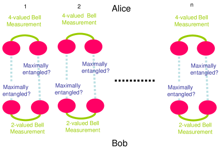
Figure 1: Asymptotic optimal testing scheme when $2n$ identical copies are given

Next, we proceed to the large deviation setting. The inequality (37) yields

$$\lim\frac{-1}{n}\log\beta_{\alpha,n,U(d^{2}-1)}^{L(A\to B)}(0\|\sigma)\geq\left\{\begin{array}[]{ll}-\log(1-p)&\hbox{ if }1-p\geq\frac{1}{d}\\ \log d&\hbox{ if }1-p\,<\frac{1}{d}\end{array}\right..$$ (42)

Hence, the relations (3) and (15) guarantee that if $1-p\geq\frac{1}{d}$,

$$\lim\frac{-1}{n}\log\beta_{\alpha,n,U(d^{2}-1)}^{L(A\to B)}(0\|\sigma)=-\log(1-p),$$

for $G=U(1),SU(d)\times U(1),U(d^{2}-1)$, $C=\emptyset,L(A\to B),L(A\leftrightarrows B),S(A,B)$. Hence, we can conclude that if $1-p\geq\frac{1}{d}$, there is no advantage of use of entanglement between ${\cal H}_{A}$ and ${\cal H}_{B}$ for this testing even in this kind of the asymptotic large deviation setting.

VII A-B locality and Sample locality

In this section, we discuss the locality among $A_{1},B_{1},\ldots,A_{n},B_{n}$. Since the case $n=1$ of this setting is the same as that of the setting section VI. Hence, we treat the case $n=2$, at first.

VII.1 Two-sample setting

We construct a level-$0$ $SU(d)$-invariant test for the null hypothesis ${\cal S}_{0}=\{|\phi^{0}_{A,B}\rangle\langle\phi^{0}_{A,B}|\}$ as follows. For this purpose, we define a POVM $M_{cov}^{1\to 2}$ on Alice’s space ${\cal H}_{A}^{\otimes 2}$, which can be realized by one-way LOCC $A_{1}\to A_{2}$ from the first system ${\cal H}_{A_{1}}$ to the second system ${\cal H}_{A_{2}}$.

Construction of $M_{cov}^{1\to 2}$: 

1) Alice performs the covariant POVM $M_{cov}^{1}$ on the first system ${\cal H}_{A_{1}}$, and obtain the data corresponding to the state $|\varphi\rangle\langle\varphi|$.

2)We choose the Projection-valued measure $\{|u^{i}(\varphi)\rangle\langle u^{i}(\varphi)|\}_{i}$ satisfying that

$$\langle u^{i}(\varphi)|u^{j}(\varphi)\rangle=0,\quad\langle u^{i}(\varphi)|\varphi\rangle=\frac{1}{\sqrt{d}}.$$ (43)

The existence of $\{u^{i}(\varphi)\}_{i}$ is shown in Appendix K.

3) Alice randomly chooses $g\in U(d-1)$ which acts on the space orthogonal to $\varphi$, and performs the Projection-valued measure $\{|gu^{i}(\varphi)\rangle\langle gu^{i}(\varphi)|\}_{i}$ on the second system ${\cal H}_{A_{2}}$.

Since Bob’s measurement of the test $T(M_{cov}^{1\to 2})$ can be also realized by one-way LOCC on Bob’s space, this test is a $L(A_{1},A_{2}\to B_{1},B_{2})$ test. Its POVM is given by

$$M_{cov}^{1\to 2}(\,dg)=d^{2}(g\otimes g)|u_{1}\otimes u_{2}\rangle\langle u_{1}\otimes u_{2}|(g\otimes g)^{\dagger}\nu(\,dg),$$

where we choose $u_{1}$ and $u_{2}$ satisfying $|\langle u_{1}|u_{2}\rangle|^{2}=\frac{1}{d}$. Thus, the $SU(d)$-covariance of $M_{cov}^{1\to 2}$ guarantees the $SU(d)$-invariance of the test $T_{inv}^{A_{1}\to A_{2}\to B^{\otimes 2}}\stackrel{{\scriptstyle\rm def}}{{=}}T(M_{cov}^{1\to 2})$. Moreover, as is shown in Appendix L, the test $T_{inv}^{A_{1}\to A_{2}\to B^{\otimes 2}}$ is $U(1)$-invariant. Hence, the inequality

$$\beta^{L(A_{1},A_{2}\to B_{1},B_{2})}_{0,2,SU(d)\times U(1)}(0\|\sigma)\leq\mathop{\rm Tr}\nolimits T_{inv}^{A_{1}\to A_{2}\to B^{\otimes 2}}\sigma^{\otimes 2}$$

holds. On the other hand, the equation

$$\beta^{L(A_{1},A_{2}\to B_{1},B_{2})}_{0,2,SU(d)}(0\|\sigma)=\mathop{\rm Tr}\nolimits T_{inv}^{A_{1}\to A_{2}\to B^{\otimes 2}}\sigma^{\otimes 2}$$ (44)

holds, which is shown in Appendix M. Hayashi et al.tsu have obtained a similar result in the two-dimensional case. Thus,

$$\beta^{L(A_{1},A_{2}\to B_{1},B_{2})}_{0,2,SU(d)}(0\|\sigma) =\beta^{L(A_{1},A_{2}\to B_{1},B_{2})}_{0,2,SU(d)\times U(1)}(0\|\sigma)$$

$$=\mathop{\rm Tr}\nolimits T_{inv}^{A_{1}\to A_{2}\to B^{\otimes 2}}\sigma^{\otimes 2}.$$

Therefore, the test $T_{inv}^{A_{1}\to A_{2}\to B^{\otimes 2}}$ is a UMP $L(A_{1},A_{2}\to B_{1},B_{2})$ $G$-invariant test with level-$0$ for the null hypothesis ${\cal S}_{0}$, where $G=SU(d),SU(d)\times U(1)$.

VII.2 $n$-sample setting

Next, we proceed to $n$-sample setting. Since the test ${T^{\prime\prime}}_{\epsilon,\alpha}^{n}\stackrel{{\scriptstyle\rm def}}{{=}}T_{\alpha}^{n}(T_{inv}^{1,A\to B},\frac{d\epsilon}{d+1})$ is level-$\alpha$ $U(d^{2}-1)$-invariant test with the hypothesis ${\cal S}_{\leq\epsilon}$, and satisfies the condition of $L(A_{1},\ldots,A_{n}\to B_{1},\ldots,B_{n})$, the inequality

$$\beta_{\alpha,n,U(d^{2}-1)}^{L(A_{1},\ldots,A_{n}\to B_{1},\ldots,B_{n})}(\leq\epsilon\|\sigma)$$

$$\leq \mathop{\rm Tr}\nolimits{T^{\prime\prime}}_{\epsilon,\alpha}^{n}\sigma^{\otimes n}=\beta_{\alpha}^{n}\left(\left.\leq\frac{d\epsilon}{d+1}\right\|\frac{dp}{d+1}\right)$$ (45)

holds.

Conversely, as a lower bound of $\beta_{\alpha,n,SU(d)}^{S(A_{1},\ldots,A_{n},B_{1},\ldots,B_{n})}(\leq\epsilon\|\sigma)$, we obtain

$$\frac{1}{n}\log\frac{\beta_{\alpha,n,SU(d)}^{S(A_{1},\ldots,A_{n},B_{1},\ldots,B_{n})}(0\|\sigma)}{1-\alpha}$$

$$\geq \min_{u,u^{\prime}:|\langle u|\overline{u^{\prime}}\rangle|=1,\|u\|=1}$$

$$\quad\int_{SU(d)}\log d\langle gu\otimes\overline{g}u^{\prime}|\sigma|gu\otimes\overline{g}u^{\prime}\rangle\nu(dg),$$ (46)

which will be shown in Appendix N.

VII.3 Asymptotic setting

Taking the limit in (45), we obtain

$$\lim\beta_{\alpha,n,U(d^{2}-1)}^{L(A_{1},\ldots,A_{n}\to B_{1},\ldots,B_{n})}\left(\left.\leq\frac{\delta}{n}\right\|\sigma_{n}\right)$$

$$\leq \beta_{\alpha}\left(\left.\leq\frac{d\delta}{d+1}\right\|\frac{dt^{\prime}}{d+1}\right)$$ (47)

if $\langle\phi^{0}_{A,B}|\sigma|\phi^{0}_{A,B}\rangle=1-\frac{t^{\prime}}{n}$. Conversely, by using the inequality (46), the compactness of the sets $\{u,u^{\prime}||\langle u|\overline{u^{\prime}}\rangle|=1,\|u\|=1\}$ and $SU(d)$ yields

$$\lim\log\frac{\beta_{\alpha,n,SU(d)}^{S(A_{1},\ldots,A_{n},B_{1},\ldots,B_{n})}(0\|\sigma_{n})}{1-\alpha}$$

$$\geq \min_{u,u^{\prime}:|\langle u|\overline{u^{\prime}}\rangle|=1,\|u\|=1}\int_{SU(d)}\lim n$$

$$\hskip 43.05542pt\log d\langle gu\otimes\overline{g}u^{\prime}|\sigma_{n}|gu\otimes\overline{g}u^{\prime}\rangle\nu(dg)$$

$$= -\min_{u,u^{\prime}:|\langle u|\overline{u^{\prime}}\rangle|=1,\|u\|=1}\int_{SU(d)}$$

$$\hskip 43.05542pt\lim n\left(1-d\langle gu\otimes\overline{g}u^{\prime}|\sigma_{n}|gu\otimes\overline{g}u^{\prime}\rangle\right)\nu(dg)$$

$$= -\min_{u,u^{\prime}:|\langle u|\overline{u^{\prime}}\rangle|=1,\|u\|=1}\lim n\mathop{\rm Tr}\nolimits(I-T_{u,u^{\prime}})\sigma_{n},$$

where

$$T_{u,u^{\prime}}\stackrel{{\scriptstyle\rm def}}{{=}}\int_{SU(d)}d|gu\otimes\overline{g}u^{\prime}\rangle\langle gu\otimes\overline{g}u^{\prime}|\nu(dg).$$

Since $T_{u,u^{\prime}}$ is $SU(d)$-invariant. The test $T_{u,u^{\prime}}$ has the form $t_{0}|\phi^{0}_{A,B}\rangle\langle\phi^{0}_{A,B}|+t_{1}(I-|\phi^{0}_{A,B}\rangle\langle\phi^{0}_{A,B}|)$. The condition $|\langle u|\overline{u^{\prime}}\rangle|=1$ guarantees that $t_{0}=1$. The definition of $T_{u,u^{\prime}}$ guarantees that $\mathop{\rm Tr}\nolimits T_{u,u^{\prime}}\geq d$, which implies $t_{1}\geq\frac{1}{d+1}$. Hence,

$$\mathop{\rm Tr}\nolimits(I-T_{u,u^{\prime}})\sigma_{n}\leq\frac{d}{d+1}\mathop{\rm Tr}\nolimits(I-|\phi^{0}_{A,B}\rangle\langle\phi^{0}_{A,B}|)\sigma_{n}$$

$$= \frac{d}{d+1}(1-\langle\phi^{0}_{A,B}|\sigma|\phi^{0}_{A,B}\rangle)=\frac{d}{d+1}\frac{t^{\prime}}{n}.$$ (48)

Thus, we have

$$\lim\log\frac{\beta_{\alpha,n,SU(d)}^{S(A_{1},\ldots,A_{n},B_{1},\ldots,B_{n})}(0\|\sigma_{n})}{1-\alpha}\geq-\frac{dt^{\prime}}{d+1},$$

which implies

$$\lim\beta_{\alpha,n,SU(d)}^{S(A_{1},\ldots,A_{n},B_{1},\ldots,B_{n})}(0\|\sigma_{n})\geq(1-\alpha)e^{-\frac{dt^{\prime}}{d+1}}.$$

Combining (47) in the case of $\epsilon$, we obtain

$$\lim\beta_{\alpha,n,G}^{S(A_{1},\ldots,A_{n},B_{1},\ldots,B_{n})}(0\|\sigma_{n})=(1-\alpha)e^{-\frac{dt^{\prime}}{d+1}}$$

for $G=SU(d),SU(d)\times U(1),U(d^{2}-1)$, $C=S(A_{1},\ldots,A_{n},B_{1},\ldots,B_{n})$, $L(A_{1},\ldots,A_{n},B_{1},\ldots,B_{n})$, $L(A_{1},\ldots,A_{n}\to B_{1},\ldots,B_{n})$. Since $(1-\alpha)e^{-\frac{dt^{\prime}}{d+1}}\,<(1-\alpha)e^{-t^{\prime}}=\beta_{\alpha}(0\|t^{\prime})$, there is an advantage to use of quantum correlation among samples.

VIII Two-sample Two-dimensional setting

Next, we proceed to the special case $n=2$ and $d=2$. For the analysis of this case, we define the $3\times 3$ real symmetric matrix $V=(v_{i,j})_{1\leq i,j\leq 3}$ as

$$v_{i,j} \stackrel{{\scriptstyle\rm def}}{{=}}\Re\langle\phi_{A,B}^{i}|\sigma|\phi_{A,B}^{j}\rangle$$

$$\phi_{A,B}^{1} \stackrel{{\scriptstyle\rm def}}{{=}}\frac{1}{\sqrt{2}}\left(|10\rangle+|10\rangle\right),\quad\phi_{A,B}^{2}\stackrel{{\scriptstyle\rm def}}{{=}}\frac{1}{\sqrt{2}}\left(-i|10\rangle+i|10\rangle\right),$$

$$\phi_{A,B}^{3} \stackrel{{\scriptstyle\rm def}}{{=}}\frac{1}{\sqrt{2}}\left(|00\rangle-|11\rangle\right).$$

When $\sigma$ satisfies the following condition $p\leq\frac{1}{2}$, as is shown in Appendix O, the equation

$$\beta_{0,2,SU(2)\times U(1)}^{C}(0\|\sigma)$$

$$= (1-p)^{2}+\frac{p^{2}}{3}-\frac{3}{5}\left(\mathop{\rm Tr}\nolimits\frac{I}{3}V^{2}-(\mathop{\rm Tr}\nolimits\frac{I}{3}V)^{2}\right)$$ (49)

holds, where $C=L(A\to B),L(A\leftrightarrows B),S(A,B)$. Since the quantity $\mathop{\rm Tr}\nolimits\frac{I}{3}V^{2}-(\mathop{\rm Tr}\nolimits\frac{I}{3}V)^{2}$ is greater than $0$, its $\frac{3}{5}$ times give the advantage of this optimal test against the test introduced in subsectionVI.2. Hence, this merit vanish if and only if the real symmetric matrix $V$ is constant. In addition, the optimal test $T$ is given as follows. First, we define a covariant POVM

$$M_{op}(dg)\stackrel{{\scriptstyle\rm def}}{{=}}4\int_{SU(2)}g^{\otimes 2}|u_{op}\rangle\langle u_{op}|(g^{\otimes 2})^{\dagger}\nu(dg),$$

where the vector $u_{op}$ is defined as

$$u_{op}\stackrel{{\scriptstyle\rm def}}{{=}} \frac{1}{2}\left(|01\rangle_{A_{1},A_{2}}-|10\rangle_{A_{1},A_{2}}\right)$$

$$\quad+\frac{\sqrt{3}}{2}\left(|00\rangle_{A_{1},A_{2}}+|11\rangle_{A_{1},A_{2}}\right).$$

Then, as is shown in Appendix O, the relation

$$\beta_{0,2,SU(2)\times U(1)}^{C}(0\|\sigma)=\mathop{\rm Tr}\nolimits T(M_{op})\sigma^{\otimes 2}$$ (50)

holds. That is, the test $T(M_{op})$ is the UMP $SU(2)\times U(1)$-invariant $C$ test with the condition $p\leq\frac{1}{2}$, where $C=L(A\to B),L(A\leftrightarrows B),S(A,B)$.

On the other hand, as is shown in Appendix P, the RHS of (44) is calculated as

$$\beta_{0,2,SU(2)}^{L(A_{1},A_{2}\to B_{1},B_{2})}(0\|\sigma)=\beta_{0,2,SU(2)\times U(1)}^{L(A_{1},A_{2}\to B_{1},B_{2})}(0\|\sigma)$$

$$= (1-\frac{2}{3}p)^{2}-\frac{1}{5}\left(\mathop{\rm Tr}\nolimits\frac{I}{3}V^{2}-(\mathop{\rm Tr}\nolimits\frac{I}{3}V)^{2}\right).$$ (51)

That is, the quantity $\frac{1}{5}\left(\mathop{\rm Tr}\nolimits\frac{I}{3}V^{2}-(\mathop{\rm Tr}\nolimits\frac{I}{3}V)^{2}\right)$ presents the effect of use of classical communication between $A_{1}$ and $A_{2}$.

IX Two different systems

In section VI, we showed that if we can prepare the two identical states simultaneously and we can perform Bell measurement on this joint system, the asymptotically optimal test can be realized. However, it is a bit difficult to prepare two identical states from the same source simultaneously. However, as is discussed in this section, if we can prepare two quantum states from the different source independently, this Bell measurement is asymptotically optimal.

IX.1 Formulation

Since the state on ${\cal H}_{A,B}^{\otimes 2}$ can be described as $\sigma_{1}\otimes\sigma_{2}$, our hypotheses are given as

$$H_{0}: \quad{\cal S}_{\leq\epsilon}^{2}\stackrel{{\scriptstyle\rm def}}{{=}}\left\{\sigma_{1}\otimes\sigma_{2}\left|\begin{array}[]{ll}(1-\langle\phi^{0}_{A,B}|\sigma_{1}|\phi^{0}_{A,B}\rangle)\\ +(1-\langle\phi^{0}_{A,B}|\sigma_{2}|\phi^{0}_{A,B}\rangle)\leq\epsilon\end{array}\right.\right\}$$

versus

$$H_{1}: \quad{\cal S}_{\leq\epsilon}^{2c}\stackrel{{\scriptstyle\rm def}}{{=}}\left\{\sigma_{1}\otimes\sigma_{2}\left|\begin{array}[]{ll}(1-\langle\phi^{0}_{A,B}|\sigma_{1}|\phi^{0}_{A,B}\rangle)\\ +(1-\langle\phi^{0}_{A,B}|\sigma_{2}|\phi^{0}_{A,B}\rangle)>\epsilon\end{array}\right.\right\}.$$

For any group action $G$ introduced in subsection III.2, these hypotheses are invariant for $G\times G$-action defined as

$$\phi\mapsto(g_{1}\otimes g_{2})\phi\quad\forall(g_{1},g_{2})\in G\times G.$$

When only two particles ${\cal H}_{A_{1},B_{1}}\otimes{\cal H}_{A_{2},B_{2}}$ are prepared, similarly to subsection III.3, we can define the quantities $\beta_{\alpha,2,G\times G}^{C}(\leq\epsilon\|\sigma_{1}\otimes\sigma_{2})$ for the condition $C=\emptyset,S(A,B),L(A\leftrightarrows B),L(A\to B),S(A_{1},A_{2},B_{1},B_{2}),L(A_{1},A_{2},B_{1},B_{2}),L(A_{1},A_{2}\to B_{1},B_{2})$, in which, “$2$” means two particles, i.e., there is only one sample of $\sigma_{1}\otimes\sigma_{2}$. When $n$ samples $(\sigma_{1}\otimes\sigma_{2})^{\otimes n}$ are prepared, we also define the quantities $\beta_{\alpha,2n,G\times G}^{C}(\leq\epsilon\|\sigma_{1}\otimes\sigma_{2})$ for the condition $C=\emptyset,S(A,B),L(A\leftrightarrows B),L(A\to B),S(A_{1},A_{2},B_{1},B_{2}),L(A_{1},A_{2},B_{1},B_{2}),L(A_{1},A_{2}\to B_{1},B_{2})$.

IX.2 One-sample setting

In this section, we treat the case of $one-sample$ and $\epsilon=0$ case. In the first step, we focus on the case of $C=\emptyset$. In this case, the relations

$$\beta_{0,2,G\times G}^{\emptyset}(0\|\sigma_{1}\otimes\sigma_{2}) =\langle\phi_{A,B}^{0}\otimes\phi_{A,B}^{0}|\sigma_{1}\otimes\sigma_{2}|\phi_{A,B}^{0}\otimes\phi_{A,B}^{0}\rangle$$

$$=(1-p_{1})(1-p_{2})$$

hold for $G=\emptyset,U(1),SU(d)\times U(1),U(d^{2}-1)$, where $p_{i}=1-\langle\phi_{A,B}^{0}|\sigma_{i}|\phi_{A,B}^{0}\rangle$.

Next, we focus on the case of $C=L(A\to B),L(A\leftrightarrows B),S(A,B)$. When we use the test $T_{inv}^{2,A\to B}$, the second error is

$$\beta(T_{inv}^{2,A\to B},\sigma_{1}\otimes\sigma_{2})=(1-p_{1})(1-p_{2})+\frac{p_{1}p_{2}}{d^{2}-1}.$$

Moreover, the optimal second error can also be calculated as

$$\beta_{0,2,G\times G}^{C}(0\|\sigma_{1}\otimes\sigma_{2})=(1-p_{1})(1-p_{2})+\frac{p_{1}p_{2}}{d^{2}-1}$$ (52)

for $C=L(A\to B),L(A\leftrightarrows B),S(A,B)$ when $\frac{p_{1}p_{2}}{d^{2}-1}\leq(1-p_{1})p_{2},p_{1}(1-p_{2})$. Its proof is given in Appendix Q. Hence, the test $T_{inv}^{2,A\to B}$ is the $C$-UMP $G$-invariant test. Using the PPT condition, Hayashi et al.tsu derived this optimal test in the case of $\sigma_{1}=\sigma_{2},d=2$.

Finally, we proceed to the case of $C=L((A_{1},A_{2})\to(B_{1},B_{2})),L(A_{1},A_{2},B_{1},B_{2}),S(A_{1},A_{2},B_{1},B_{2})$. When we use the test $T_{inv}^{1,A_{1}\to B_{1}}\otimes T_{inv}^{1,A_{2}\to B_{2}}$, the second error is

$$\beta(T_{inv}^{1,A_{1}\to B_{1}}\otimes T_{inv}^{1,A_{2}\to B_{2}},\sigma_{1}\otimes\sigma_{2})$$

$$= \left(1-\frac{dp_{1}}{d+1}\right)\left(1-\frac{dp_{2}}{d+1}\right).$$

In this case, as is proven in Appendix R, the optimal second error is calculated as

$$\beta_{0,2,G\times G}^{C}(0\|\sigma_{1}\otimes\sigma_{2})=\left(1-\frac{dp_{1}}{d+1}\right)\left(1-\frac{dp_{2}}{d+1}\right),$$ (53)

for $G=SU(d),SU(d)\times U(1),U(d^{2}-1)$. Thus, the test $T_{inv}^{1,A_{1}\to B_{1}}\otimes T_{inv}^{1,A_{2}\to B_{2}}$ is the $C$-UMP $G$-invariant test. Hayashi et al.tsu derived this optimal test in the case of $\sigma_{1}=\sigma_{2},d=2$.

IX.3 Asymptotic setting

In the small deviation asymptotic setting with $n$ samples, we focus on the case $\epsilon=\frac{\delta}{n}$ and $\frac{t_{i}^{\prime}}{n}=1-\langle\phi_{A,B}^{0}|\sigma_{i,n}^{\prime}|\phi_{A,B}^{0}\rangle$. In this setting, as is shown in Appendix S,

$$\lim\beta_{\alpha,2n,G\times G}^{\emptyset}(\leq\frac{\delta}{n}\|\sigma_{1,n}^{\prime}\otimes\sigma_{2,n}^{\prime})=\beta_{\alpha}(\leq\delta\|t_{1}^{\prime}+t_{2}^{\prime})$$ (54)

for $G=U(1),SU(d)\times U(1),U(d^{2}-1)$.

Next, we consider the case of $C=L(A\to B)$. When we perform the test $T_{inv}^{2,A\to B}$ for all systems ${\cal H}_{A_{1}}\otimes{\cal H}_{B_{1}},\ldots,{\cal H}_{A_{n}}\otimes{\cal H}_{B_{n}}$ whose state is $\sigma_{1,n}^{\prime}\otimes\sigma_{2,n}^{\prime}$, the number $k$ of detecting $T_{inv}^{2,A\to B}$ almost obeys the Poisson distribution $e^{-(t_{1}^{\prime}+t_{2}^{\prime})}\frac{(t_{1}^{\prime}+t_{2}^{\prime})^{k}}{k!}$. This is because $n\left(1-(1-\frac{t_{1}^{\prime}}{n})(1-\frac{t_{2}^{\prime}}{n})+\frac{\frac{t_{1}^{\prime}}{n}\frac{t_{2}^{\prime}}{n}}{d^{2}-1}\right)\to t_{1}^{\prime}+t_{2}^{\prime}$. Treating the hypothesis testing of this Poisson distribution, we can show that the $L(A\to B)$ $U(d^{2}-1)\times U(d^{2}-1)$-invariant test $T^{n,2}_{\epsilon,\alpha}\stackrel{{\scriptstyle\rm def}}{{=}}T_{\alpha}^{n}(T_{inv}^{2,A\to B},\max_{p_{1}+p_{2}=\epsilon}p_{1}+p_{2}-\frac{d^{2}p_{1}p_{2}}{d^{2}-1})$ satisfies that

$$\lim\beta(T^{n,2}_{\delta/n,\alpha},\sigma_{1,n}^{\prime}\otimes\sigma_{2,n}^{\prime})=\beta_{\alpha}(\leq\delta\|t_{1}^{\prime}+t_{2}^{\prime}).$$

Hence, combining (54), we obtain

$$\lim\beta_{\alpha,2n,G\times G}^{C}\left(\left.\leq\frac{\delta}{n}\right\|\sigma_{1,n}^{\prime}\otimes\sigma_{2,n}^{\prime}\right)=\beta_{\alpha}(\leq\delta\|t_{1}^{\prime}+t_{2}^{\prime}).$$

for $C=\emptyset,L(A\to B),L(A\leftrightarrows B),S(A,B)$, $G=SU(d)\times U(1),U(d^{2}-1)$. Therefore, the test $T^{n,2}_{\epsilon,\alpha}$ is $C$-UMP $G$-invariant test in the asymptotic small deviation setting. The asymptotic optimal testing scheme is illustrated as Fig. 2.

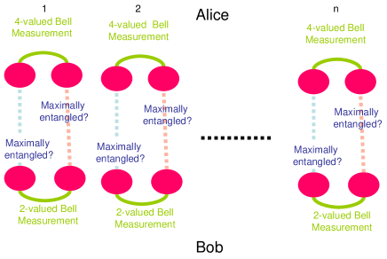
Figure 2: Asymptotic optimal testing scheme when $n$ identical copies are given and one sample system consists of two different systems

Moreover, if we use the test based on the Bell measurement in stead of the test $T_{inv}^{2,A\to B}$, the bound $\beta_{\alpha}(\leq\delta\|t_{1}^{\prime}+t_{2}^{\prime})$ can be attained because of a reason similar to Lemma 5.

X Three different systems

Finally, we treat the case of three quantum states are prepared independently. Similarly to section IX.1, we put two hypotheses

$$H_{0}: ~{}{\cal S}_{\leq\epsilon}^{3}\stackrel{{\scriptstyle\rm def}}{{=}}\left\{\bigotimes_{i=1}^{3}\sigma_{i}\left|1-\sum_{i=1}^{3}\langle\phi^{0}_{A_{i},B_{i}}|\sigma_{i}|\phi^{0}_{A_{i},B_{i}}\rangle\leq\epsilon\right.\right\}$$

versus

$$H_{1}: ~{}{\cal S}_{\leq\epsilon}^{3c}\stackrel{{\scriptstyle\rm def}}{{=}}\left\{\bigotimes_{i=1}^{3}\sigma_{i}\left|1-\sum_{i=1}^{3}\langle\phi^{0}_{A_{i},B_{i}}|\sigma_{i}|\phi^{0}_{A_{i},B_{i}}\rangle>\epsilon\right.\right\},$$

where the given state is assumed to be $\sigma_{1}\otimes\sigma_{2}\otimes\sigma_{3}$. Similarly we define the quantities $\beta_{\alpha,3,G\times G\times G}^{C}(\leq\epsilon\|\sigma_{1}\otimes\sigma_{2}\otimes\sigma_{3})$ for the condition $C=\emptyset,S(A,B),L(A\leftrightarrows B),L(A\to B),L((A_{1},A_{2},A_{3})\to(B_{1},B_{2},B_{3})),L(A_{1},A_{2},A_{3},B_{1},B_{2},B_{3})$, $S(A_{1},A_{2},A_{3},B_{1},B_{2},B_{3})$ under the similar $G\times G\times G$-invariance.

Similarly to subsection IX.2, we focus on the case of $C=L(A\to B),L(A\leftrightarrows B),S(A,B)$ with one sample. In this case, as is mentioned, the GHZ state $|GHZ\rangle\stackrel{{\scriptstyle\rm def}}{{=}}\frac{1}{\sqrt{d}}\sum_{i=0}^{d-1}|i\rangle_{A_{1}}|i\rangle_{A_{2}}|i\rangle_{A_{3}}$ plays an important role. Since the $SU(d)\times SU(d)\times SU(d)$-action on ${\cal H}_{A_{1}}\otimes{\cal H}_{A_{2}}\otimes{\cal H}_{A_{3}}$ is irreducible, the following is a POVM:

$$M_{cov}^{3}(dg_{1},dg_{2},dg_{3})$$

$$\stackrel{{\scriptstyle\rm def}}{{=}} d^{3}g_{1}\otimes g_{2}\otimes g_{3}|GHZ\rangle\langle GHZ|(g_{1}\otimes g_{2}\otimes g_{3})^{\dagger}$$

$$\quad\nu(dg_{1})\nu(dg_{2})\nu(dg_{3}).$$

As is proved in Appendix T, the test $T_{inv}^{3,A\to B}\stackrel{{\scriptstyle\rm def}}{{=}}T(M_{cov}^{3})$ has the form

$$T_{inv}^{3,A\to B}$$

$$= P_{1}\otimes P_{2}\otimes P_{3}+\frac{(d+2)P_{1}^{c}\otimes P_{2}^{c}\otimes P_{3}^{c}}{(d+1)^{3}(d-1)}$$

$$\quad+\frac{P_{1}\otimes P_{2}^{c}\otimes P_{3}^{c}+P_{1}^{c}\otimes P_{2}\otimes P_{3}^{c}+P_{1}^{c}\otimes P_{2}^{c}\otimes P_{3}}{(d+1)^{2}(d-1)},$$ (55)

where $P_{i}=|\phi_{A_{i},B_{i}}^{0}\rangle\langle\phi_{A_{i},B_{i}}^{0}|,P_{i}^{c}=I-P_{i}$. Thus, this test is $U(d^{2}-1)\times U(d^{2}-1)\times U(d^{2}-1)$-invariant. Hence, when we use the test $T_{inv}^{3,A\to B}$, the second error is

$$\beta(T_{inv}^{3,A\to B},\sigma_{1}\otimes\sigma_{2}\otimes\sigma_{3})$$

$$= (1-p_{1})(1-p_{2})(1-p_{3})+\frac{(d+2)p_{1}p_{2}p_{3}}{(d+1)^{2}(d-1)}$$

$$\quad+\frac{p_{1}p_{2}(1-p_{3})+p_{1}(1-p_{2})p_{3}+(1-p_{1})p_{2}p_{3}}{(d+1)^{2}(d-1)}.$$

Moreover, the optimal second error can be also calculated as

$$\beta_{0,3,G\times G\times G}^{C}(0\|\sigma_{1}\otimes\sigma_{2}\otimes\sigma_{3})$$

$$= (1-p_{1})(1-p_{2})(1-p_{3})+\frac{(d+2)p_{1}p_{2}p_{3}}{(d+1)^{2}(d-1)}$$

$$\quad+\frac{p_{1}p_{2}(1-p_{3})+p_{1}(1-p_{2})p_{3}+(1-p_{1})p_{2}p_{3}}{(d+1)^{2}(d-1)}$$ (56)

for $C=L(A\to B),L(A\leftrightarrows B),S(A,B)$ when $p_{i}\leq\frac{d-1}{d}$. Its proof is given in Appendix T. Hence, the test $T_{inv}^{3,A\to B}$ is the $C$-UMP $G$-invariant test.

On the other hand, the case of $C=L(A_{1},A_{2},A_{3}\to B_{1},B_{2},B_{3})$, $L(A_{1},A_{2},A_{3},B_{1},B_{2},B_{3})$, $S(A_{1},A_{2},A_{3},B_{1},B_{2},B_{3})$. Similarly to (53), we can show the optimality of the test $T_{inv}^{1,A\to B}\otimes T_{inv}^{1,A\to B}\otimes T_{inv}^{1,A\to B}$. Moreover, we can derive the same result in the small deviation asymptotic setting with $n$ samples.

XI Conclusion

In this paper, we treated the hypotheses testing problem when the null hypothesis consists only of the required entangled state or is its neighboor hood. In order to treat the structure of entanglement, we consider three settings concerning the range of accessible measurements as follows: M1: All measurements are allowed. M2: A measurement is forbidden if it requires the quantum correlation between two distinct parties. M3: A measurement is forbidden if it requires the quantum correlation between two distinct parties, or that among local samples. As a result, we found that there is difference between the accuracies of M1 and M2 in the first order asymptotics. The protocol achieving the asymtotic bound has been proposed in the setting M2. In this setting, it is required to prepare two identical samples at the same time. However, it is difficult to prepare the two states from the same source. In order to avoid this difficulty, we proved that even if the two states is prepared from the different source, this proposed protocol works effectively. In particular, this protocol can be realized in the two-dimensional system if the four-valued Bell measurement can be realized. Moreover, concerning the finite samples case, we derived optimal testing in several examples. Thus, as was demonstrated by Hayashi et al. exper , it is a future target to demonstrate the proposed testing experimentally.

In this paper, the optimal test is constructed based on continuous valued POVM. However, any realizable POVM is finite valued. Hence, it is desired to construct the optimal test based on the finite valued POVM. This problem is partially discussed by Hayashi et al., and will be more deeply discussed by another paper ha1 .

The obtained protocol is essentially equivalent with the following procedure based on the quantum teleportation. First, we perform quantum teleportation from the system $A$ to the system $B$, which succeed when the true state is the required maximally entangled state. Next, we check whether the state on the system $B$ is the initial state on the system $A$. Hence, an interesting relation between the obtained results and the quantum teleportation is expected, and it will be treated in a forthcoming paper ha2 .

As a related research, the following testing problem has been discussed LC ; BS . Assume that $N$ qubits state are given, and we can measure only $M$ qubits. The required problem is testing whether the remaining $N-M$ qubits are the desired maximally entangled state. Indeed, this problem is important not only for gurarantee of the quality of the prepared maximally entangled state, but also for the security for the quantum key distribution. The problem discussed in this paper is different from the preceding probelem in testing the given state by measuring the whole system. In order to apply our result to the preceding problem, we have to randomly choose $M$ qubits among the given $N$ qubits, and test the $N$ qubits. When the given $N$ qubits do not satisfy the independent and identical condition, their method LC ; BS is better than our method. Since their method LC ; BS requires the the quantum correlation among whole $M$ qubits, it is difficult to realize their method for testing the prepared maximally entangled state, but it is possible to apply their method to testing the security of quantum key distribution LC . This is because the maximally entangled state is only virtually discussed in the latter case. Hence, for testing the prepared maximally entangled state, it is natural from the practical viewpoint to restrict our test among random sampling method. Since our results can be applied this setting, they can be expected to be applied to the check of the quality of maximally entangled state.

As another problem, Acín et al. acin-tarrach-vidal discussed the problem testing whether the given $n$-i.i.d. state of the unknown pure state is the $n$-tensor product of a pure maximally entangled state (not the specific maximally entangled state) in the two-dimensional system. This problem is closely related to universal entanglement concentrationMH . Its $d$-dimensional case is a future problem.

Appendix A Proof of Lemma 1 and Lemma 2

Assume that a set of test satisfying the condition $C$ is invariant for the action of $G_{2}$. Let $T\in{\cal T}_{\alpha,\leq\epsilon}^{n}$ be a test satisfying the condition $C$, then the test $\overline{T}\stackrel{{\scriptstyle\rm def}}{{=}}(f(g)^{\dagger})^{\otimes n}Tf(g)^{\otimes n}$ also satisfies the condition $C$ and belongs to the set ${\cal T}_{\alpha,\leq\epsilon}^{n}$. Since

$$\beta(T,(f(g)\sigma f(g)^{\dagger})^{\otimes n})=\beta(f(g)^{\dagger}Tf(g),\sigma^{\otimes n}),$$

we obtain

$$\max_{g\in G}\beta(T,(f(g)\sigma f(g)^{\dagger})^{\otimes n})$$

$$\geq \int_{G_{2}}\beta(T,(f(g)\sigma f(g)^{\dagger})^{\otimes n})\nu_{G}(dg)$$

$$= \beta(\overline{T},(f(g)\sigma f(g)^{\dagger})^{\otimes n})\geq\beta_{\alpha,n,G_{2}}^{C}(\leq\epsilon\|\sigma).$$

Hence,

$$\min_{T\in{\cal T}_{\alpha,\leq\epsilon}^{n}}\max_{g\in G}\beta(T,(f(g)\sigma f(g)^{\dagger})^{\otimes n})$$

$$\geq\min_{T\in{\cal T}_{\alpha,\leq\epsilon}^{n}}\int_{G}\beta(T,(f(g)\sigma f(g)^{\dagger})^{\otimes n})\nu_{G}(dg)$$

$$\geq\beta_{\alpha,n,G}^{C}(\leq\epsilon\|\sigma).$$ (57)

On the other hand, if the $G_{2}$-invariant test $T\in{\cal T}_{\alpha,\leq\epsilon}^{n}$ satisfies the condition $C$ and

$$\beta(T,\sigma^{\otimes n})=\beta_{\alpha,n,G_{2}}^{C}(\leq\epsilon\|\sigma),$$

then

$$\beta(T,(f(g)\sigma f(g)^{\dagger})^{\otimes n})$$

$$= \beta(T,\sigma^{\otimes n})=\beta_{\alpha,n,G_{2}}^{C}(\leq\epsilon\|\sigma)\quad\forall g\in G_{2},$$

which implies

$$\max_{g\in G}\beta(T,(f(g)\sigma f(g)^{\dagger})^{\otimes n})=\beta_{\alpha,n,G_{2}}^{C}(\leq\epsilon\|\sigma).$$

Thus, we obtain the inequality opposite to (57). Therefore, the proof of Lemma 1 is completed.

Next, we proceed to prove Lemma 2. Since the equation

$$\int_{G_{1}}\beta(T,(f(g)\sigma f(g)^{\dagger})^{\otimes n})\nu_{G_{1}}(dg)$$

$$= \int_{G_{1}}\beta((f(g^{\prime})^{\dagger})^{\otimes n}Tf(g^{\prime})^{\otimes n},(f(g)\sigma f(g)^{\dagger})^{\otimes n})\nu_{G_{1}}(dg)$$

holds for $\forall g^{\prime}\in G_{2}$, we obtain

$$\min_{T\in{\cal T}_{\alpha,\leq\epsilon}^{n}}\max_{g\in G_{1}}\beta(T,(f(g)\sigma f(g)^{\dagger})^{\otimes n})$$

$$\geq\min_{T\in{\cal T}_{\alpha,\leq\epsilon}^{n}}\int_{G_{1}}\beta(T,(f(g)\sigma f(g)^{\dagger})^{\otimes n})\nu_{G_{1}}(dg)$$

$$=\min_{T\in{\cal T}_{\alpha,\leq\epsilon}^{n}}\int_{G_{2}}\int_{G_{1}}\beta((f(g^{\prime})^{\dagger})^{\otimes n}Tf(g^{\prime})^{\otimes n},(f(g)\sigma f(g)^{\dagger})^{\otimes n})$$

$$\hskip 21.52771pt\nu_{G_{1}}(dg)\nu_{G_{2}}(dg^{\prime})$$

$$=\min_{T\in{\cal T}_{\alpha,\leq\epsilon}^{n}}\int_{G_{1}}\beta((\overline{T},(f(g)\sigma f(g)^{\dagger})^{\otimes n})\nu_{G_{1}}(dg)$$

$$\geq\int_{G_{1}}\beta_{\alpha,n,G_{2}}^{C}(\leq\epsilon\|f(g)\sigma f(g)^{\dagger})\nu_{G_{1}}(dg)$$

$$=\int_{G_{1}}\beta_{\alpha,n,G_{1}}^{C}(\leq\epsilon\|f(g)\sigma f(g)^{\dagger})\nu_{G_{1}}(dg).$$ (58)

Since $\beta(T^{\prime},\sigma)=\beta(T^{\prime},f(g)\sigma f(g)^{\dagger})$ for any $G_{1}$-invariant test $T^{\prime}$, we have

$$\beta_{\alpha,n,G_{1}}^{C}(\leq\epsilon\|\sigma)=\beta_{\alpha,n,G_{1}}^{C}(\leq\epsilon\|f(g)\sigma f(g)^{\dagger}),$$

which implies

$$\int_{G_{1}}\beta_{\alpha,n,G_{1}}^{C}(\leq\epsilon\|f(g)\sigma f(g)^{\dagger})\nu_{G_{1}}(dg)=\beta_{\alpha,n,G_{1}}^{C}(\leq\epsilon\|\sigma).$$

We choose a $G_{1}$-invariant test $T\in{\cal T}_{\alpha,\leq\epsilon}^{n}$ satisfying the condition $C$ and

$$\beta_{\alpha,n,G_{1}}^{C}(\leq\epsilon\|\sigma)=\beta(T,\sigma).$$

Then,

$$\max_{g\in G_{1}}\beta(T,(f(g)\sigma f(g)^{\dagger})^{\otimes n})=\beta(T,\sigma)=\beta_{\alpha,n,G_{1}}^{C}(\leq\epsilon\|\sigma).$$

Thus, we obtain the inequality opposite to (58), which yields Lemma 2.

Appendix B Basic properties of classical tests

In the classical hypotheses testing, Neymann Pearson Lemma plays a central role.

Lemma 6

Assume that the null hypothesis is one probability distribution $P_{0}$ and the alternative one is another probability distribution $P_{1}$. For any $\,>\alpha\,>0$, we choose $r$ and $\gamma$ such that

$$P_{0}\left\{x\left|\frac{P_{0}(x)}{P_{1}(x)}\,>r\right.\right\} \leq 1-\alpha$$

$$P_{0}\left\{x\left|\frac{P_{0}(x)}{P_{1}(x)}\,<r\right.\right\} \leq\alpha$$

$$\gamma P_{0}\left\{x\left|\frac{P_{0}(x)}{P_{1}(x)}=r\right.\right\} =1-\alpha-P_{0}\left\{x\left|\frac{P_{0}(x)}{P_{1}(x)}\,>r\right.\right\},$$

and define the test $\tilde{T}_{P_{0},P_{1},\alpha}$ as

$$\tilde{T}_{P_{0},P_{1},\alpha}(x)=\left\{\begin{array}[]{ll}1&\hbox{ if }\frac{P_{0}(x)}{P_{1}(x)}\,>r\\ \gamma&\hbox{ if }\frac{P_{0}(x)}{P_{1}(x)}=r\\ 0&\hbox{ if }\frac{P_{0}(x)}{P_{1}(x)}\,<r.\end{array}\right.$$ (62)

Then, the test $T_{P_{0},P_{1},\alpha}$ is the MP level-$\alpha$ test.

In classical statistics, the function $\frac{P_{0}(x)}{P_{1}(x)}$ is called the likelihood ratio, which plays an important role.

Proof: Assume that $\tilde{T}^{*}$ is a level-$\alpha$ test. We focus on the weighted sum of two kinds of error probabilities $\sum_{x}P_{0}(x)(1-\tilde{T}^{*}(x))+r\sum_{x}P_{1}(x)\tilde{T}^{*}(x)$. Since $\sum_{x}(P_{0}(x)-rP_{1}(x))\tilde{T}^{*}(x)\leq\sum_{x}(P_{0}(x)-rP_{1}(x))\tilde{T}_{r}(x)$, we can see

$$\sum_{x}P_{0}(x)(1-\tilde{T}^{*}(x))+r\sum_{x}P_{1}(x)\tilde{T}^{*}(x)$$

$$= 1-\sum_{x}(P_{0}(x)-rP_{1}(x))\tilde{T}^{*}(x)$$

$$\geq 1-\sum_{x}(P_{0}(x)-rP_{1}(x))\tilde{T}_{P_{0},P_{1},\alpha}(x)$$

$$= \sum_{x}P_{0}(x)(1-\tilde{T}_{P_{0},P_{1},\alpha}(x))+r\sum_{x}P_{1}(x)\tilde{T}_{P_{0},P_{1},\alpha}(x).$$

Hence, the relation $\sum_{x}P_{0}(x)(1-\tilde{T}^{*}(x))=\sum_{x}P_{0}(x)(1-\tilde{T}_{P_{0},P_{1},\alpha}(x))=\alpha$ yields that

$$\sum_{x}P_{1}(x)\tilde{T}^{*}(x)\geq\sum_{x}P_{1}(x)\tilde{T}_{P_{0},P_{1},\alpha}(x).$$

 

We have the following corollary.

Corollary 2

If the test $\tilde{T}$ has the form (62), i.e., a likelihood ratio test, then the inequality

$$\sum_{x}P_{0}(x)(1-\tilde{T}(x))\leq\sum_{x}P_{1}(x)(1-\tilde{T}(x))$$

holds.

Proof: We focus on the test $\tilde{T}^{\prime}(x)\stackrel{{\scriptstyle\rm def}}{{=}}1-\alpha$. Since the test $\tilde{T}^{\prime}$ is trivially level-$\alpha$, Lemma 6 guarantees that $\sum_{x}P_{1}(x)\tilde{T}(x)\leq\sum_{x}P_{1}(x)\tilde{T}^{\prime}(x)=1-\alpha$, which implies that $\sum_{x}P_{0}(x)(1-\tilde{T}(x))=\alpha\leq\sum_{x}P_{1}(x)(1-\tilde{T}(x))$.   

Appendix C Proof of Theorem 1

Since the likelihood ratio $\frac{P_{\epsilon}^{n}(k)}{P_{q}^{n}(k)}$ is the monotone decreasing function of $k$, the test $\tilde{T}_{\epsilon,\alpha}$ equals the test $\tilde{T}_{P_{\epsilon}^{n},P_{q}^{n},\alpha}$. Lemma 6 guarantees that the test $\tilde{T}_{\epsilon,\alpha}$ is the MP level-$\alpha$ test with the null hypothesis $P_{\epsilon}^{n}$. Since a level-$\alpha$ test with the null hypothesis ${\cal P}^{n}_{\leq\epsilon}$ is a level-$\alpha$ test with the null hypothesis $P_{\epsilon}^{n}$,

$$\beta_{\alpha}^{n}(\leq\epsilon\|q)\geq P_{q}^{n}(\tilde{T}_{\epsilon,\alpha}).$$ (63)

Since the likelihood ratio $\frac{P_{p_{0}}^{n}(k)}{P_{p_{1}}^{n}(k)}$ is the monotone decreasing function of $k$ for $p_{0}\,<p_{1}$, the test $\tilde{T}_{\epsilon,\alpha}$ is a likelihood ratio test of $P_{p_{0}}^{n}$ and $P_{p_{1}}^{n}$. Hence, Corollary 2 guarantees that $P_{p_{0}}^{n}(\tilde{T}_{\epsilon,\alpha})\geq P_{p_{1}}^{n}(\tilde{T}_{\epsilon,\alpha})$. That is, the probability $P_{p}^{n}(\tilde{T}_{\epsilon,\alpha})$ is a monotone decreasing function of $p$. Since the definition of the test $\tilde{T}_{\epsilon,\alpha}$ implies that $P_{\epsilon}^{n}(\tilde{T}_{\epsilon,\alpha})=1-\alpha$, $P_{p}^{n}(\tilde{T}_{\epsilon,\alpha})\leq 1-\alpha$ if $p\leq\epsilon$. In other words, the test $\tilde{T}_{\epsilon,\alpha}$ is level-$\alpha$ with the null hypothesis ${\cal P}^{n}_{\leq\epsilon}$. Hence, it follows from the inequality (63) that the test $\tilde{T}_{\epsilon,\alpha}$ is level-$\alpha$ UMP test with the null hypothesis ${\cal P}^{n}_{\leq\epsilon}$.

Appendix D Proof of Theorem 2

Since $\tilde{T}_{\delta/n,\alpha}^{n}$ is a level-$\alpha$ test the null hypothesis ${\cal P}_{\frac{\delta}{n}}$, $\forall t\in[0,\delta]\quad\limsup 1-\sum_{k}P_{t}(k)\tilde{T}_{\delta/n,\alpha}^{n}(k)=\limsup 1-\sum_{k}P_{t/n}^{n}(k)\tilde{T}_{\delta/n,\alpha}^{n}(k)\leq\alpha$. Hence, for $\forall\epsilon\,>0$ there exists $N$ such that $\forall n\geq N,\forall t\in[0,\delta]\quad 1-P_{t}(\tilde{T}_{\delta/n,\alpha}^{n})\leq\alpha+\epsilon$. Hence,

$$P_{t^{\prime}}(\tilde{T}_{\delta/n,\alpha}^{n})\geq\beta_{\alpha+\epsilon}(\leq\delta\|t^{\prime})$$

Since $\liminf P_{t^{\prime}}(\tilde{T}_{\delta/n,\alpha}^{n})=\liminf P_{t^{\prime}/n}^{n}(\tilde{T}_{\delta/n,\alpha}^{n})=\liminf\beta^{n}_{\alpha}\left(\leq\frac{\delta}{n}\left\|\frac{t^{\prime}}{n}\right.\right)$,

$$\liminf\beta^{n}_{\alpha}\left(\leq\frac{\delta}{n}\left\|\frac{t^{\prime}}{n}\right.\right)\geq\beta_{\alpha+\epsilon}(\leq\delta\|t^{\prime}).$$

Since the continuity of $\alpha\mapsto\beta_{\alpha}(\leq\delta\|t^{\prime})$ follows from Theorem 3,

$$\liminf\beta^{n}_{\alpha}\left(\leq\frac{\delta}{n}\left\|\frac{t^{\prime}}{n}\right.\right)\geq\beta_{\alpha}(\leq\delta\|t^{\prime}).$$

Since $\tilde{T}_{\delta,\alpha-\epsilon}$ is level-$\alpha$ test the null hypothesis $t\in[0,\delta]$ for $\forall\epsilon\,>0$, we have $\forall t\in[0,\delta]\quad\limsup 1-\sum_{k}P_{t/n}^{n}(k)\tilde{T}_{\delta,\alpha-\epsilon}(k)=\limsup 1-\sum_{k}P_{t}(k)\tilde{T}_{\delta,\alpha-\epsilon}(k)\leq\alpha-\epsilon$. Hence, there exists $N$ such that $\forall n\geq N,\forall t\in[0,\delta]\quad 1-P_{t/n}^{n}(\tilde{T}_{\delta,\alpha-\epsilon})\leq\alpha$. Hence,

$$P_{t^{\prime}/n}^{n}(\tilde{T}_{\delta,\alpha-\epsilon})\geq\beta_{\alpha}^{n}(\leq\delta/n\|t^{\prime}/n)$$

Thus,

$$\beta_{\alpha}^{n}(\leq\delta/n\|t^{\prime}/n)\leq\beta_{\alpha-\epsilon}(\leq\delta\|t^{\prime}),$$

which implies

$$\limsup\beta_{\alpha}^{n}(\leq\delta/n\|t^{\prime}/n)\leq\beta_{\alpha-\epsilon}(\leq\delta\|t^{\prime}).$$

The continuity of $\alpha\mapsto\beta_{\alpha}(\leq\delta\|t^{\prime})$ guarantees that

$$\limsup\beta_{\alpha}^{n}(\leq\delta/n\|t^{\prime}/n)\leq\beta_{\alpha}(\leq\delta\|t^{\prime}).$$

Appendix E Proof of (9)

For a fixed density matrix $\sigma$ on ${\cal H}_{A,B}$, we define a density matrix $\sigma_{q}$ as

$$\sigma_{q} \stackrel{{\scriptstyle\rm def}}{{=}}\left(\sqrt{\frac{1-q}{1-p}}|\phi^{0}_{A,B}\rangle\langle\phi^{0}_{A,B}|+\sqrt{\frac{q}{p}}(I-|\phi^{0}_{A,B}\rangle\langle\phi^{0}_{A,B}|)\right)\cdot$$

$$\quad\sigma\left(\sqrt{\frac{1-q}{1-p}}|\phi^{0}_{A,B}\rangle\langle\phi^{0}_{A,B}|+\sqrt{\frac{q}{p}}(I-|\phi^{0}_{A,B}\rangle\langle\phi^{0}_{A,B}|)\right),$$

where $p\stackrel{{\scriptstyle\rm def}}{{=}}1-\langle\phi^{0}_{A,B}|\sigma|\phi^{0}_{A,B}\rangle$. We also define the matrix $\sigma^{\prime}$ by

$$\frac{1}{p}(I-|\phi^{0}_{A,B}\rangle\langle\phi^{0}_{A,B}|)\sigma(I-|\phi^{0}_{A,B}\rangle\langle\phi^{0}_{A,B}|).$$

Let $T$ be a $U(1)$-invariant test with level-$\alpha$. The $U(1)$-invariance yields that

$$\mathop{\rm Tr}\nolimits T(U_{\theta}^{\otimes n})^{\dagger}\rho_{q}^{\otimes n}U_{\theta}^{\otimes n}=\mathop{\rm Tr}\nolimits U_{\theta}^{\otimes n}T(U_{\theta}^{\otimes n})^{\dagger}\rho_{q}^{\otimes n}=\mathop{\rm Tr}\nolimits T\rho_{q}^{\otimes n}.$$

Hence,

$$\mathop{\rm Tr}\nolimits T\rho_{q}^{\otimes n}=\frac{1}{2\pi}\int_{0}^{2\pi}\mathop{\rm Tr}\nolimits T(U_{\theta}^{\otimes n})^{\dagger}\rho_{q}^{\otimes n}U_{\theta}^{\otimes n}\,d\theta=\mathop{\rm Tr}\nolimits T\overline{\rho}_{q}^{n},$$ (64)

where we define $\overline{\rho}_{\theta}$ as

$$\overline{\rho}_{q}^{n} \stackrel{{\scriptstyle\rm def}}{{=}}\frac{1}{2\pi}\int_{0}^{2\pi}(U_{\theta}^{\otimes n})^{\dagger}\rho_{q}^{\otimes n}U_{\theta}^{\otimes n}\,d\theta$$

$$=\sum_{k=0}^{n}q^{k}(1-q)^{n-k}P_{k}^{n}(|\phi^{0}_{A,B}\rangle\langle\phi^{0}_{A,B}|,\sigma^{\prime}).$$

Thus, the test $T$ is a level-$\alpha$ test with the null hypothesis $\overline{\rho}_{\epsilon}^{n}$.

In the following, we focus on the hypotheses testing with the null hypothesis $\overline{\rho}_{\epsilon}^{n}$ and the alternative hypothesis $\overline{\rho}_{p}^{n}$. Since these two states are commutative with each other, there exists a basis $\{e_{k,l}\}$ diagonalizing them. As they are written as $\overline{\rho}_{\epsilon}=\sum_{k}\sum_{l}P^{k,l}_{0}|e_{k,l}\rangle\langle e_{k,l}|$ and $\overline{\rho}_{p}=\sum_{k}\sum_{l}P^{k,l}_{1}|e_{k,l}\rangle\langle e_{k,l}|$, our problem is essentially equivalent with the classical hypothesis testing with the null hypothesis $P_{0}\stackrel{{\scriptstyle\rm def}}{{=}}(P_{0}^{k,l})$ and the alternative hypothesis $P_{1}\stackrel{{\scriptstyle\rm def}}{{=}}(P_{1}^{k,l})$. Since the likelihood ratio is given by the ratio $\frac{\epsilon^{k}(1-\epsilon)^{n-k}}{p^{k}(1-p)^{n-k}}$, we have

$$T^{n}_{\epsilon,\alpha}=\sum_{k}\sum_{l}\tilde{T}_{P_{0},P_{1},\alpha}|e_{k,l}\rangle\langle e_{k,l}|.$$

Hence, Lemma 6 guarantees that

$$\mathop{\rm Tr}\nolimits T\overline{\rho}_{p}^{n}\geq T^{n}_{\epsilon,\alpha}\overline{\rho}_{p}^{n}$$

because the test $T$ is a level-$\alpha$ test with the null hypothesis $\overline{\rho}_{\epsilon}^{n}$. Since $T^{n}_{\epsilon,\alpha}$ is $U(1)$-invariant, the equation (64) guarantees that

$$\mathop{\rm Tr}\nolimits T\sigma^{\otimes n}\geq T^{n}_{\epsilon,\alpha}\sigma^{\otimes n}.$$

The equation $T^{n}_{\epsilon,\alpha}\sigma^{\otimes n}=\beta_{\alpha}^{n}(\leq\epsilon\|p)$ yields (9).

Appendix F Proof of Lemma 3

Let $T$ be a one-way LOCC $(A\to B)$ level-$0$ test with the null hypothesis $|\phi^{0}_{A,B}\rangle\langle\phi^{0}_{A,B}|$. We denote Alice’s first measurement by $M=\{M_{i}\}$. In this case, Bob’s measurement can be described by two-valued measurement $\{T_{0}^{i},I-T_{0}^{i}\}$, where $T_{0}^{i}$ corresponds to the decision accepting the state $|\phi^{0}_{A,B}\rangle\langle\phi^{0}_{A,B}|$. Hence the test $T$ can be described as

$$T=\sum_{i}M_{i}\otimes T_{0}^{i}.$$

When Alice observes the data $i$, the Bob’s state is $\frac{1}{\mathop{\rm Tr}\nolimits\overline{M_{i}}}\overline{M_{i}}$. Since this test is level-$0$,

$$T_{0}^{i}\geq P_{i},$$

where $P_{i}$ is the projection to the range of the matrix $\overline{M_{i}}$.

Here, we diagonalize $M_{i}$ as $M_{i}=\sum_{j}p_{i,j}|u_{i,j}\rangle\langle u_{i,j}|$. Since $P_{i}\geq|\overline{u_{i,j}}\rangle\langle\overline{u_{i,j}}|$, the POVM $M^{\prime}=\{p_{i,j}|u_{i,j}\rangle\langle u_{i,j}|\}_{i,j}$, satisfies

$$T(M^{\prime}) =\sum_{i,j}p_{i,j}|u_{i,j}\otimes\overline{u_{i,j}}\rangle\langle u_{i,j}\otimes\overline{u_{i,j}}|$$

$$=\sum_{i,j}p_{i,j}|u_{i,j}\rangle\langle u_{i,j}|\otimes|\overline{u_{i,j}}\rangle\langle\overline{u_{i,j}}|$$

$$\leq\sum_{i,j}p_{i,j}|u_{i,j}\rangle\langle u_{i,j}|\otimes P_{i}=\sum_{i}M_{i}\otimes P_{i}$$

$$\leq\sum_{i}M_{i}\otimes T_{0}^{i}=T.$$

Appendix G Proof of Lemma 4

It follows from the condition (21) that $\sum_{i}p_{i}=1$. We choose the vector $\varphi\stackrel{{\scriptstyle\rm def}}{{=}}\sqrt{d}\sum_{i}p_{i}u_{i}\otimes{u^{\prime}}_{i}$. Since the function $x\to|x|^{2}$ is convex, we obtain

$$\langle\varphi|T|\varphi\rangle\geq d\sum_{i}p_{i}\langle\varphi|u_{i}\otimes{u^{\prime}}_{i}\rangle\langle u_{i}\otimes{u^{\prime}}_{i}|\varphi\rangle$$

$$= d\sum_{i}p_{i}|\langle\varphi|u_{i}\otimes{u^{\prime}}_{i}\rangle|^{2}\geq d|\sum_{i}p_{i}\langle\varphi|u_{i}\otimes{u^{\prime}}_{i}\rangle|^{2}$$

$$= d\left|\frac{1}{\sqrt{d}}\langle\varphi|\varphi\rangle\right|^{2}=\|\varphi\|^{4}.$$

Hence,

$$1\geq\mathop{\rm Tr}\nolimits T\frac{|\varphi\rangle\langle\varphi|}{\|\varphi\|^{2}}=\|\varphi\|^{2}.$$

On the other hand,

$$\langle\phi^{0}_{A,B}|\varphi\rangle=\sqrt{d}\sum_{i}p_{i}\langle\phi^{0}_{A,B}|u_{i}\otimes{u^{\prime}}_{i}\rangle=1.$$

Since $\|\phi^{0}_{A,B}\|=1$, we obtain

$$\varphi=\phi^{0}_{A,B}.$$

Appendix H Proof of (23)

The representation space ${\cal H}_{A}\otimes{\cal H}_{B}$ of $SU(d)$-action can be irreducibly decomposed to two subspaces: One is the one-dimensional space $<\phi^{0}_{A,B}>$ spanned by $\phi^{0}_{A,B}$. The other is its orthogonal space $<\phi^{0}_{A,B}>^{\perp}$. Since the $T_{inv}^{1,A\to B}$ is $SU(d)$-invariant, it has the form

$$T_{inv}^{1,A\to B}=t_{0}|\phi^{0}_{A,B}\rangle\langle\phi^{0}_{A,B}|+t_{1}(I-|\phi^{0}_{A,B}\rangle\langle\phi^{0}_{A,B}|).$$

The equation $\langle\phi^{0}_{A,B}|T_{inv}^{1,A\to B}|\phi^{0}_{A,B}\rangle=1$ implies $t_{0}=1$. Its trace can be calculated as

$$\mathop{\rm Tr}\nolimits T_{inv}^{1,A\to B}=\int d\mathop{\rm Tr}\nolimits|\varphi\otimes\overline{\varphi}\rangle\langle\varphi\otimes\overline{\varphi}|\nu(\,d\varphi)=d.$$

Hence, $t_{1}=\frac{d-1}{d^{2}-1}=\frac{1}{d+1}$.

Appendix I Proof of (27)

Lemma 7

If the test $T$ is a separable on the space ${\cal H}_{A}\otimes{\cal H}_{B}$, then

$$\mathop{\rm Tr}\nolimits T\geq d\langle\phi^{0}_{A,B}|T|\phi^{0}_{A,B}\rangle,$$ (65)

where $d$ is the dimension of ${\cal H}_{A}$.

Proof: Since $T$ is separable, $T$ has the form $T=\sum_{l}|u_{i}\otimes u^{\prime}_{i}\rangle\langle u_{i}\otimes u^{\prime}_{i}|$. For any two vectors $u,u^{\prime}$, Schwarz inequality yields that

$$\langle u\otimes u^{\prime}|u\otimes u^{\prime}\rangle =\langle u|u\rangle\langle u^{\prime}|u^{\prime}\rangle=\langle u|u\rangle\langle\overline{u^{\prime}}|\overline{u^{\prime}}\rangle\geq|\langle u|\overline{u^{\prime}}\rangle|^{2}$$

$$=d|\langle\phi_{A,B}^{0}|u\otimes u^{\prime}\rangle|^{2}.$$

Hence, we have

$$\mathop{\rm Tr}\nolimits|u_{i}\otimes u^{\prime}_{i}\rangle\langle u_{i}\otimes u^{\prime}_{i}|\geq d\langle\phi^{0}_{A,B}|u_{i}\otimes u^{\prime}_{i}\rangle\langle u_{i}\otimes u^{\prime}_{i}|\phi^{0}_{A,B}\rangle.$$

Taking the sum, we obtain (65).   

Assume that $T$ is a $SU(d)$-invariant separable test. From the discussion in section H, the test $T$ has the form

$$T=t_{0}|\phi^{0}_{A,B}\rangle\langle\phi^{0}_{A,B}|+t_{1}(I-|\phi^{0}_{A,B}\rangle\langle\phi^{0}_{A,B}|).$$

Lemma 7 implies that $t_{1}(d^{2}-1)+t_{0}\geq dt_{0}$, i.e., $t_{1}\geq\frac{1}{d+1}t_{0}$. Hence, the test $T$ has another form

$$T= t_{0}^{\prime}\left(|\phi^{0}_{A,B}\rangle\langle\phi^{0}_{A,B}|+\frac{1}{d+1}(I-|\phi^{0}_{A,B}\rangle\langle\phi^{0}_{A,B}|)\right)$$

$$+t_{1}^{\prime}\frac{d}{d+1}(I-|\phi^{0}_{A,B}\rangle\langle\phi^{0}_{A,B}|)$$

$$= t_{0}^{\prime}T_{inv}^{1,A\to B}+t_{1}^{\prime}(I-T_{inv}^{1,A\to B}).$$

Since

$$\mathop{\rm Tr}\nolimits\sigma T_{inv}^{1,A\to B}=1-\frac{dp}{d+1},\quad\mathop{\rm Tr}\nolimits\sigma(I-T_{inv}^{1,A\to B})=\frac{dp}{d+1},$$

our problem is equivalent with the hypotheses testing concerning the probability $(1-\frac{dp}{d+1},\frac{dp}{d+1})$. Thus, we obtain (27).

Appendix J Proof of Lemma 5 and (31)

Lemma 8

A state $u\in{\cal H}_{A_{1}}\otimes{\cal H}_{A_{2}}$ is maximally entangled if and only if

$$|\phi^{0}_{A_{1},B_{1}}\rangle\langle\phi^{0}_{A_{1},B_{1}}|\otimes(I-|\phi^{0}_{A_{2},B_{2}}\rangle\langle\phi^{0}_{A_{2},B_{2}}|)u\otimes\overline{u} =0$$ (66)

$$(I-|\phi^{0}_{A_{1},B_{1}}\rangle\langle\phi^{0}_{A_{1},B_{1}}|)\otimes|\phi^{0}_{A_{2},B_{2}}\rangle\langle\phi^{0}_{A_{2},B_{2}}|u\otimes\overline{u} =0.$$ (67)

Proof: The condition (66) equivalent to the condition that $\langle\phi^{0}_{A_{1},B_{1}}|u\otimes\overline{u}\rangle$ equals the constant times of $|\phi^{0}_{A_{2},B_{2}}\rangle$. When we choose a matrix $U$ as $u=\sum_{i,j}\frac{U_{i,j}}{\sqrt{d}}|i\rangle_{A_{1}}|j\rangle_{A_{2}}$, this condition equals to the condition that $UIU^{\dagger}$ is a constant matrix. Thus, if and only if $u$ is maximally entangled, $U$ is unitary, which is equivalent with the condition (66). Similarly, we can show that the maximally entangledness of $u$ equivalent with the condition (67). Hence, the desired argument is proved.   

The relations (17) and (18) guarantee that $\phi^{0}_{A_{1},B_{1}}\otimes\phi^{0}_{A_{2},B_{2}}$ is an eigenvector of $T(M)$ with the eigenvalue $1$. Hence, Lemma 8 implies (33). On the other hand,

$$\mathop{\rm Tr}\nolimits P\sigma^{\otimes 2}P=\left(\mathop{\rm Tr}\nolimits\sigma(I-|\phi^{0}_{A_{1},B_{1}}\rangle\langle\phi^{0}_{A_{1},B_{1}}|)\right)^{2}$$

$$= \left(1-\langle\phi^{0}_{A_{1},B_{1}}|\sigma|\phi^{0}_{A_{1},B_{1}}\rangle\right)^{2}.$$

Since $0\leq PT(M)P\leq I$, we obtain (35).

Next, we consider the case of $M=M^{2}_{cov}$. The test $T(M^{2}_{cov})$ is invariant the following action, i.e.,

$$U(g_{1})\otimes U(g_{2})T(M^{2}_{cov})(U(g_{1})\otimes U(g_{2}))^{\dagger}=T(M^{2}_{cov})$$

Since the subspace $<\phi^{0}_{A_{1},B_{1}}>^{\perp}\otimes<\phi^{0}_{A_{2},B_{2}}>^{\perp}$ is irreducible subspace, the equation (33) implies

$$T(M^{2}_{cov})=|\phi^{0}_{A_{1},B_{1}}\otimes\phi^{0}_{A_{2},B_{2}}\rangle\langle\phi^{0}_{A_{1},B_{1}}\otimes\phi^{0}_{A_{2},B_{2}}|+tP,$$

where $t$ is a constant. Since the equation (19) implies that $\mathop{\rm Tr}\nolimits T(M^{2}_{cov})=d^{2}$, we obtain $t=\frac{d^{2}-1}{(d^{2}-1)^{2}}=\frac{1}{d^{2}-1}$.

Appendix K Proof of (43)

We focus on the vertex of the simplex of the $d-1$-dimensional subspace orthogonal to $\varphi$. That is, there exist $d$ vectors $u_{1}(\varphi),\ldots,u_{d}(\varphi)$ such that

$$\langle u_{i}(\varphi)|u_{j}(\varphi)\rangle=\left\{\begin{array}[]{ll}-\frac{1}{d}&i\neq j\\ \frac{d-1}{d}&i=j.\end{array}\right.$$

Hence, the $d$ vectors $u^{i}(\varphi)\stackrel{{\scriptstyle\rm def}}{{=}}u_{i}(\varphi)+\frac{1}{\sqrt{d}}\varphi$ satisfy the condition (43).

Appendix L Proof of the $U(1)$-invariance of $T_{inv}^{1\to 2}$

As is proved later, the test $T_{inv}^{1\to 2}$ has the form

$$T_{inv}^{A_{1}\to A_{2}\to B^{\otimes 2}}$$

$$= d^{2}\int_{G}(g\otimes\overline{g})\otimes(g\otimes\overline{g})|u_{1}\otimes\overline{u_{1}}\otimes u_{2}\otimes\overline{u_{2}}\rangle\langle u_{1}\otimes\overline{u_{1}}\otimes u_{2}\otimes\overline{u_{2}}|(g\otimes\overline{g})^{\dagger}\otimes(g\otimes\overline{g})^{\dagger}\nu(\,dg)$$

$$= d^{2}\int_{G}(g\otimes\overline{g})\otimes(g\otimes\overline{g})\Biggl{(}\left|\frac{1}{d^{2}}\phi_{A_{1},B_{1}}^{0}\otimes\phi_{A_{2},B_{2}}^{0}\right\rangle\left\langle\frac{1}{d^{2}}\phi_{A_{1},B_{1}}^{0}\otimes\phi_{A_{2},B_{2}}^{0}\right|$$

$$+\left|\frac{1}{d}\phi_{A_{1},B_{1}}^{0}\otimes\left(u_{2}\otimes\overline{u_{2}}-\frac{1}{d}\phi_{A_{2},B_{2}}^{0}\right)\right\rangle\left\langle\frac{1}{d}\phi_{A_{1},B_{1}}^{0}\otimes\left(u_{2}\otimes\overline{u_{2}}-\frac{1}{d}\phi_{A_{2},B_{2}}^{0}\right)\right|$$

$$+\left|\left(u_{1}\otimes\overline{u_{1}}-\frac{1}{d}\phi_{A_{1},B_{1}}^{0}\right)\otimes\frac{1}{d}\phi_{A_{2},B_{2}}^{0}\right\rangle\left\langle\left(u_{1}\otimes\overline{u_{1}}-\frac{1}{d}\phi_{A_{1},B_{1}}^{0}\right)\otimes\frac{1}{d}\phi_{A_{2},B_{2}}^{0}\right|$$

$$+\left|\left(u_{1}\otimes\overline{u_{1}}-\frac{1}{d}\phi_{A_{1},B_{1}}^{0}\right)\otimes\left(u_{2}\otimes\overline{u_{2}}-\frac{1}{d}\phi_{A_{2},B_{2}}^{0}\right)\right\rangle\left\langle\left(u_{1}\otimes\overline{u_{1}}-\frac{1}{d}\phi_{A_{1},B_{1}}^{0}\right)\otimes\left(u_{2}\otimes\overline{u_{2}}-\frac{1}{d}\phi_{A_{2},B_{2}}^{0}\right)\right|$$

$$\hskip 43.05542pt\Biggr{)}(g\otimes\overline{g})^{\dagger}\otimes(g\otimes\overline{g})^{\dagger}\nu(\,dg).$$ (68)

Thus, we can easily check that the matrix $T_{inv}^{1\to 2}$ is commutative with the matrix

$$U_{\theta}^{\otimes 2}= e^{2\theta i}|\phi_{A_{1},B_{1}}^{0}\rangle\langle\phi_{A_{1},B_{1}}^{0}|\otimes|\phi_{A_{2},B_{2}}^{0}\rangle\langle\phi_{A_{2},B_{2}}^{0}|$$

$$+e^{\theta i}\left(|\phi_{A_{1},B_{1}}^{0}\rangle\langle\phi_{A_{1},B_{1}}^{0}|\otimes\left(I_{A_{2},B_{2}}-|\phi_{A_{2},B_{2}}^{0}\rangle\langle\phi_{A_{2},B_{2}}^{0}|\right)+\left(I_{A_{1},B_{1}}-|\phi_{A_{1},B_{1}}^{0}\rangle\langle\phi_{A_{1},B_{1}}^{0}|\right)\otimes|\phi_{A_{2},B_{2}}^{0}\rangle\langle\phi_{A_{2},B_{2}}^{0}|\right)$$

$$+\left(I_{A_{1},B_{1}}-|\phi_{A_{1},B_{1}}^{0}\rangle\langle\phi_{A_{1},B_{1}}^{0}|\right)\otimes\left(I_{A_{2},B_{2}}-|\phi_{A_{2},B_{2}}^{0}\rangle\langle\phi_{A_{2},B_{2}}^{0}|\right).$$

, we obtain $U(1)$-invariance.

Next, we prove (68). Since

$$u_{1}\otimes\overline{u_{1}}\otimes u_{2}\otimes\overline{u_{2}}$$

$$= \frac{1}{d^{2}}\phi_{A_{1},B_{1}}^{0}\otimes\phi_{A_{2},B_{2}}^{0}+\frac{1}{d}\phi_{A_{1},B_{1}}^{0}\otimes\left(u_{2}\otimes\overline{u_{2}}-\frac{1}{d}\phi_{A_{2},B_{2}}^{0}\right)$$

$$+\left(u_{1}\otimes\overline{u_{1}}-\frac{1}{d}\phi_{A_{1},B_{1}}^{0}\right)\otimes\frac{1}{d}\phi_{A_{2},B_{2}}^{0}+\left(u_{1}\otimes\overline{u_{1}}-\frac{1}{d}\phi_{A_{1},B_{1}}^{0}\right)\otimes\left(u_{2}\otimes\overline{u_{2}}-\frac{1}{d}\phi_{A_{2},B_{2}}^{0}\right),$$

it is sufficient to prove that the integrals of the cross terms equal to $0$. We denote the invariant subgroup of $u$ by $G_{u}$ and its invariant measure by $\nu_{u}$. Then, we can calculate

$$\int_{G_{u_{1}}}(g^{\prime}\otimes\overline{g^{\prime}})\left(u_{2}\otimes\overline{u_{2}}-\frac{1}{d}\phi_{A_{2},B_{2}}^{0}\right)\nu_{u}(dg^{\prime})=\frac{1}{d}\phi_{A_{2},B_{2}}^{0}-\frac{1}{d}\phi_{A_{2},B_{2}}^{0}=0.$$

Hence, the integral of one cross term can be calculated as

$$d^{2}\int_{G}(g\otimes\overline{g})\otimes(g\otimes\overline{g})\left|\left(u_{1}\otimes\overline{u_{1}}-\frac{1}{d}\phi_{A_{1},B_{1}}^{0}\right)\right\rangle\left\langle\left(u_{1}\otimes\overline{u_{1}}-\frac{1}{d}\phi_{A_{1},B_{1}}^{0}\right)\right|\otimes$$

$$\hskip 43.05542pt\left|\frac{1}{d}\phi_{A_{2},B_{2}}^{0}\right\rangle\left\langle\left(u_{2}\otimes\overline{u_{2}}-\frac{1}{d}\phi_{A_{2},B_{2}}^{0}\right)\right|(g\otimes\overline{g})^{\dagger}\otimes(g\otimes\overline{g})^{\dagger}\nu(dg)$$

$$= d^{2}\int_{G}(g\otimes\overline{g})\left|\left(u_{1}\otimes\overline{u_{1}}-\frac{1}{d}\phi_{A_{1},B_{1}}^{0}\right)\right\rangle\left\langle\left(u_{1}\otimes\overline{u_{1}}-\frac{1}{d}\phi_{A_{1},B_{1}}^{0}\right)\right|(g\otimes\overline{g})^{\dagger}\otimes$$

$$\hskip 43.05542pt\int_{G_{u_{1}}}(g^{\prime}\otimes\overline{g^{\prime}})\left|\frac{1}{d}\phi_{A_{2},B_{2}}^{0}\right\rangle\left\langle\left(u_{2}\otimes\overline{u_{2}}-\frac{1}{d}\phi_{A_{2},B_{2}}^{0}\right)\right|(g^{\prime}\otimes\overline{g^{\prime}})^{\dagger}\nu_{u_{1}}(dg^{\prime})\nu(dg)$$

$$= 0.$$

Similarly, we can check that the integrals of other cross term is $0$.

Appendix M Proof of (44)

Let $T$ be an $SU(d)$-invariant $L(A_{1},A_{2}\to B_{1},B_{2})$ test with level-$0$. Using the discussion of Proof of Lemma 3, we can find a POVM $M^{\prime}=\{d^{2}|u_{x}^{1}\otimes u_{x}^{2}\rangle\langle u_{x}^{1}\otimes u_{x}^{2}|\mu(dx)\}$ satisfying the condition (20), where $\mu$ is a probability measure. We define the covariant POVM $M$ as

$$M(dgdx)=d^{2}|g^{\otimes 2}u_{x}^{1}\otimes u_{x}^{2}\rangle\langle g^{\otimes 2}u_{x}^{1}\otimes u_{x}^{2}|\nu(dg)\mu(dx).$$

The $SU(d)$-invariance of $T$ guarantees that

$$T\geq\int_{SU(d)}U(g)^{\otimes 2}T(M^{\prime})(U(g)^{\otimes 2})^{\dagger}\nu(dg)=T(M).$$

Note test $T(M)$ can be expressed as

$$T(M)= \int\int_{SU(d)}d^{2}|U(g)u_{x}^{1}\otimes\overline{u_{x}^{1}}\rangle\langle U(g)u_{x}^{1}\otimes\overline{u_{x}^{1}}|$$

$$\otimes|U(g)u_{x}^{2}\otimes\overline{u_{x}^{2}}\rangle\langle U(g)u_{x}^{2}\otimes\overline{u_{x}^{2}}|\nu(dg)\mu(dx).$$ (69)

Thus, we can restrict our tests to the tests $T(M)$ with the form (69). First, we calculate the following value:

$$\mathop{\rm Tr}\nolimits\int_{SU(d)} |U(g)u_{x}^{1}\otimes\overline{u_{x}^{1}}\rangle\langle U(g)u_{x}^{1}\otimes\overline{u_{x}^{1}}|$$

$$\otimes|U(g)u_{x}^{2}\otimes\overline{u_{x}^{2}}\rangle\langle U(g)u_{x}^{2}\otimes\overline{u_{x}^{2}}|\nu(dg)\sigma^{\otimes 2}.$$

Indeed, from the $SU(d)$-invariance, this value depends only on the inner product $r\stackrel{{\scriptstyle\rm def}}{{=}}|\langle u_{x}^{1},u_{x}^{2}\rangle|^{2}$. Hence, we can denote it by $f(r)$. Without loss of generality, we can assume that $u_{x}^{1}=|0\rangle$,$u_{x}^{2}=\sqrt{p}|0\rangle+\sqrt{1-p}|1\rangle$. The group $SU(d)$ has the subgroup:

$$G^{\prime}\stackrel{{\scriptstyle\rm def}}{{=}}\left\{\left.g_{\theta}\stackrel{{\scriptstyle\rm def}}{{=}}e^{i\theta/2}|0\rangle\langle 0|+e^{-i\theta/2}|1\rangle\langle 1|+\sum_{i=2}^{d-1}|i\rangle\langle i|\right|\theta\in[0,2\pi]\right\}.$$

Hence,

$$\int_{0}^{2\pi}|U(g_{\theta})u_{x}^{1}\otimes\overline{u_{x}^{1}}\rangle\langle U(g_{\theta})u_{x}^{1}\otimes\overline{u_{x}^{1}}|\otimes|U(g_{\theta})u_{x}^{2}\otimes\overline{u_{x}^{2}}\rangle\langle U(g_{\theta})u_{x}^{2}\otimes\overline{u_{x}^{2}}|d\theta$$

$$= |00\rangle\langle 00|\otimes\Bigl{(}p(1-p)|01\rangle\langle 01|+p(1-p)|10\rangle\langle 10|$$

$$+(p|00\rangle+(1-p)|11\rangle\langle 00|)(p\langle 00|+(1-p)\langle 11|\langle 00|)\Bigr{)}$$

$$= |00\rangle\langle 00|\otimes\Bigl{(}p(1-p)|10\rangle\langle 10|+p(1-p)|01\rangle\langle 01|$$

$$+p^{2}|00\rangle\langle 00|+p(1-p)(|00\rangle\langle 11|+|11\rangle\langle 00|)+(1-p)^{2}|11\rangle\langle 11|\Bigr{)}$$

$$= |00\rangle\langle 00|\otimes\Bigl{(}|11\rangle\langle 11|+p^{2}\left(-|01\rangle\langle 01|-|10\rangle\langle 10|+|00\rangle\langle 00|+|11\rangle\langle 11|-|00\rangle\langle 11|-|11\rangle\langle 00|\right)$$

$$+p\left(|01\rangle\langle 01|+|10\rangle\langle 10|-2|11\rangle\langle 11|+|00\rangle\langle 11|+|11\rangle\langle 00|\right)\Bigr{)}.$$

We put

$$C_{1}(\sigma) \stackrel{{\scriptstyle\rm def}}{{=}}\int_{SU(d)}\langle 00|U(g)\sigma U(g)^{\dagger}|00\rangle\Bigl{(}-\langle 01|U(g)\sigma U(g)^{\dagger}|01\rangle-\langle 10|U(g)\sigma U(g)^{\dagger}|10\rangle+\langle 00|U(g)\sigma U(g)^{\dagger}|00\rangle$$

$$\hskip 86.11084pt+\langle 11|U(g)\sigma U(g)^{\dagger}|11\rangle-\langle 11|U(g)\sigma U(g)^{\dagger}|00\rangle-\langle 00|U(g)\sigma U(g)^{\dagger}|11\rangle\Bigr{)}\nu(dg)$$

$$C_{2}(\sigma) \stackrel{{\scriptstyle\rm def}}{{=}}\int_{SU(d)}\langle 00|U(g)\sigma U(g)^{\dagger}|00\rangle\Bigl{(}\langle 01|U(g)\sigma U(g)^{\dagger}|01\rangle+\langle 10|U(g)\sigma U(g)^{\dagger}|10\rangle$$

$$\hskip 86.11084pt-2\langle 11|U(g)\sigma U(g)^{\dagger}|11\rangle+\langle 11|U(g)\sigma U(g)^{\dagger}|00\rangle+\langle 00|U(g)\sigma U(g)^{\dagger}|11\rangle\Bigr{)}\nu(dg)$$

$$C_{3}(\sigma) \stackrel{{\scriptstyle\rm def}}{{=}}\int_{SU(d)}\langle 00|U(g)\sigma U(g)^{\dagger}|00\rangle\langle 11|U(g)\sigma U(g)^{\dagger}|11\rangle\nu(dg).$$

Hence, putting $p(x)\stackrel{{\scriptstyle\rm def}}{{=}}|\langle u_{x}^{1}|u_{x}^{2}\rangle|^{2}$, we have

$$\mathop{\rm Tr}\nolimits T(M)\sigma^{\otimes 2}$$

$$= \int d^{2}\left(C_{1}(\sigma)p(x)^{2}+C_{2}(\sigma)p(x)+C_{3}(\sigma)\right)\mu(dx).$$

Denoting the projection to the symmetric subspace of ${\cal H}_{A}^{\otimes 2}$ by $P_{S}$, we obtain

$$\frac{d(d+1)}{2}=\mathop{\rm Tr}\nolimits P_{S}IP_{S}$$

$$= \int\int_{SU(d)}d^{2}\mathop{\rm Tr}\nolimits P_{S}|gu_{x}^{1}\otimes gu_{x}^{2}\rangle\langle gu_{x}^{1}\otimes gu_{x}^{2}|P_{S}\nu(dg)\mu(dx)$$

$$= \int\int_{SU(d)}d^{2}\frac{1+|\langle gu_{x}^{1}|gu_{x}^{2}\rangle|^{2}}{2}\nu(dg)\mu(dx)$$

$$= \int d^{2}\frac{1+|\langle u_{x}^{1}|u_{x}^{2}\rangle|^{2}}{2}\mu(dx),$$

which implies

$$\int p(x)\mu(dx)=\frac{1}{d}$$

because $|\langle u_{x}^{1}|u_{x}^{2}\rangle|^{2}=p(x)$. As is shown later, $C_{1}(\sigma)$ is positive. Since $\int p(x)^{2}\mu(dx)\geq\frac{1}{d^{2}}$,

$$\mathop{\rm Tr}\nolimits T(M)\sigma^{\otimes 2}\geq d^{2}\left(\frac{C_{1}(\sigma)}{d^{2}}+\frac{C_{2}(\sigma)}{d}+C_{3}(\sigma)\right).$$

The equality holds if $p(x)=\frac{1}{d}$ for all $x$. That is, if $T=T_{inv}^{1\to 2}$, the equality holds. Therefore, we obtain (44).

Letting

$$g^{\prime}=\left(\begin{array}[]{ccc}0&-1&\\ 1&0&\\ &&I\end{array}\right)g,$$

we obtain

$$\int_{SU(d)}\langle 00|U(g)\sigma U(g)^{\dagger}|00\rangle\Bigl{(}-\langle 01|U(g)\sigma U(g)^{\dagger}|01\rangle-\langle 10|U(g)\sigma U(g)^{\dagger}|10\rangle+\langle 00|U(g)\sigma U(g)^{\dagger}|00\rangle$$

$$\hskip 86.11084pt+\langle 11|U(g)\sigma U(g)^{\dagger}|11\rangle-\langle 11|U(g)\sigma U(g)^{\dagger}|00\rangle-\langle 00|U(g)\sigma U(g)^{\dagger}|11\rangle\Bigr{)}\nu(dg)$$

$$= \int_{SU(d)}\langle 11|U(g^{\prime})\sigma U(g^{\prime})^{\dagger}|11\rangle\Bigl{(}-\langle 01|U(g^{\prime})\sigma U(g^{\prime})^{\dagger}|01\rangle-\langle 10|U(g^{\prime})\sigma U(g^{\prime})^{\dagger}|10\rangle+\langle 00|U(g^{\prime})\sigma U(g^{\prime})^{\dagger}|00\rangle$$

$$\hskip 86.11084pt+\langle 11|U(g^{\prime})\sigma U(g^{\prime})^{\dagger}|11\rangle-\langle 11|U(g^{\prime})\sigma U(g^{\prime})^{\dagger}|00\rangle-\langle 00|U(g^{\prime})\sigma U(g^{\prime})^{\dagger}|11\rangle\Bigr{)}\nu(dg^{\prime}).$$

Hence,

$$C_{1}(\sigma)= \int_{SU(d)}\frac{1}{2}\left(\langle 00|U(g)\sigma U(g)^{\dagger}|00\rangle+\langle 11|U(g)\sigma U(g)^{\dagger}|11\rangle\right)$$

$$\hskip 64.58313pt\Bigl{(}-\langle 01|U(g)\sigma U(g)^{\dagger}|01\rangle-\langle 10|U(g)\sigma U(g)^{\dagger}|10\rangle+\langle 00|U(g)\sigma U(g)^{\dagger}|00\rangle$$

$$\hskip 86.11084pt+\langle 11|U(g)\sigma U(g)^{\dagger}|11\rangle-\langle 11|U(g)\sigma U(g)^{\dagger}|00\rangle-\langle 00|U(g)\sigma U(g)^{\dagger}|11\rangle\Bigr{)}\nu(dg).$$ (70)

By using the notations

$$\varphi_{A,B}^{0}\stackrel{{\scriptstyle\rm def}}{{=}}\frac{1}{\sqrt{2}}\left(|00\rangle+|11\rangle\right),\quad\varphi_{A,B}^{1}\stackrel{{\scriptstyle\rm def}}{{=}}\frac{1}{\sqrt{2}}\left(|10\rangle+|10\rangle\right),\quad\varphi_{A,B}^{2}\stackrel{{\scriptstyle\rm def}}{{=}}\frac{1}{\sqrt{2}}\left(-i|10\rangle+i|10\rangle\right),\quad\varphi_{A,B}^{3}\stackrel{{\scriptstyle\rm def}}{{=}}\frac{1}{\sqrt{2}}\left(|00\rangle-|11\rangle\right),$$

$C_{1}(\sigma)$ can be calculated as

$$C_{1}(\sigma)= \int_{SU(d)}\frac{1}{2}\left(\langle\phi_{A,B}^{0}|U(g)\sigma U(g)^{\dagger}|\phi_{A,B}^{0}\rangle+\langle\phi_{A,B}^{3}|U(g)\sigma U(g)^{\dagger}|\phi_{A,B}^{3}\rangle\right)$$

$$\hskip 43.05542pt\Bigl{(}2\langle\phi_{A,B}^{3}|U(g)\sigma U(g)^{\dagger}|\phi_{A,B}^{3}\rangle-\langle\phi_{A,B}^{1}|U(g)\sigma U(g)^{\dagger}|\phi_{A,B}^{1}\rangle-\langle\phi_{A,B}^{2}|U(g)\sigma U(g)^{\dagger}|\phi_{A,B}^{2}\rangle\Bigr{)}\nu(dg).$$

Similarly to (70), focusing the elements $g_{1,2},g_{2,3},g_{3,1}$ of $SU(d)$ such that

$$g_{1,2}: (\phi_{A,B}^{1},\phi_{A,B}^{2},\phi_{A,B}^{3})\to(\phi_{A,B}^{2},-\phi_{A,B}^{1},\phi_{A,B}^{3})$$

$$g_{2,3}: (\phi_{A,B}^{1},\phi_{A,B}^{2},\phi_{A,B}^{3})\to(\phi_{A,B}^{1},\phi_{A,B}^{3},-\phi_{A,B}^{2})$$

$$g_{3,1}: (\phi_{A,B}^{1},\phi_{A,B}^{2},\phi_{A,B}^{3})\to(-\phi_{A,B}^{3},\phi_{A,B}^{2},\phi_{A,B}^{1}),$$

we can prove

$$C_{1}(\sigma)= \int_{SU(d)}\frac{1}{3}\left(\sum_{i=1}^{3}\langle\phi_{A,B}^{i}|U(g)\sigma U(g)^{\dagger}|\phi_{A,B}^{i}\rangle^{2}-\sum_{i>j}\langle\phi_{A,B}^{i}|U(g)\sigma U(g)^{\dagger}|\phi_{A,B}^{i}\rangle\langle\phi_{A,B}^{j}|U(g)\sigma U(g)^{\dagger}|\phi_{A,B}^{j}\rangle\right)\nu(dg)$$

$$= \int_{SU(d)}\frac{1}{6}\sum_{i>j}\left(\langle\phi_{A,B}^{i}|U(g)\sigma U(g)^{\dagger}|\phi_{A,B}^{i}\rangle-\langle\phi_{A,B}^{j}|U(g)\sigma U(g)^{\dagger}|\phi_{A,B}^{j}\rangle\right)^{2}\nu(dg)\geq 0.$$

Appendix N Proof of (46)

Let $T$ be a $SU(d)$-invariant separable level-$\alpha$ test among $A_{1},\ldots,A_{n},B_{1},\ldots,B_{n}$ with the null hypothesis ${\cal S}_{0}$. Then, $T$ has the following form:

$$T=\sum_{k}a_{k}|u_{1}^{k}\otimes{u^{\prime}}_{1}^{k}\rangle\langle u_{1}^{k}\otimes{u^{\prime}}_{1}^{k}|\otimes\cdots\otimes|u_{n}^{k}\otimes{u^{\prime}}_{n}^{k}\rangle\langle u_{n}^{k}\otimes{u^{\prime}}_{n}^{k}|,$$

where $\|u_{i}^{k}\|=1,\langle u_{i}^{k}|{u^{\prime}}_{i}^{k}\rangle=1$. Since $T$ is level-$\alpha$ and $\langle\phi_{A,B}^{0}||u_{1}^{k}\otimes{u^{\prime}}_{1}^{k}\rangle\langle u_{1}^{k}\otimes{u^{\prime}}_{1}^{k}||\phi_{A,B}^{0}\rangle=\frac{1}{d}$, we have

$$1-\alpha=\langle{\phi_{A,B}^{0}}^{\otimes n}|T|{\phi_{A,B}^{0}}^{\otimes n}\rangle=\sum_{k}a_{k}\frac{1}{d^{n}}.$$

It follows from the $SU(d)$-invariance of $T$ that

$$T= \int_{SU(d)}\sum_{k}a_{k}|gu_{1}^{k}\otimes\overline{g}{u^{\prime}}_{1}^{k}\rangle\langle gu_{1}^{k}\otimes\overline{g}{u^{\prime}}_{1}^{k}|$$

$$\quad\otimes\cdots\otimes|gu_{n}^{k}\otimes\overline{g}{u^{\prime}}_{n}^{k}\rangle\langle gu_{n}^{k}\otimes\overline{g}{u^{\prime}}_{n}^{k}|\nu(dg).$$

The concavity of the function $x\mapsto\log x$ implies that

$$\log\mathop{\rm Tr}\nolimits\Biggl{(}\int_{SU(d)}|gu_{1}^{k}\otimes\overline{g}{u^{\prime}}_{1}^{k}\rangle\langle gu_{1}^{k}\otimes\overline{g}{u^{\prime}}_{1}^{k}|\otimes\cdots$$

$$\quad\otimes|gu_{n}^{k}\otimes\overline{g}{u^{\prime}}_{n}^{k}\rangle\langle gu_{n}^{k}\otimes\overline{g}{u^{\prime}}_{n}^{k}|\nu(dg)\Biggr{)}\sigma^{\otimes n}$$

$$= \log\int_{SU(d)}\mathop{\rm Tr}\nolimits\langle gu_{1}^{k}\otimes\overline{g}{u^{\prime}}_{1}^{k}|\sigma|gu_{1}^{k}\otimes\overline{g}{u^{\prime}}_{1}^{k}\rangle$$

$$\quad\cdots\mathop{\rm Tr}\nolimits\langle gu_{n}^{k}\otimes\overline{g}{u^{\prime}}_{n}^{k}|\sigma|gu_{n}^{k}\otimes\overline{g}{u^{\prime}}_{n}^{k}\rangle\nu(dg)$$

$$\geq \int_{SU(d)}\sum_{i=1}^{n}\log\mathop{\rm Tr}\nolimits\langle gu_{i}^{k}\otimes\overline{g}{u^{\prime}}_{i}^{k}|\sigma|gu_{i}^{k}\otimes\overline{g}{u^{\prime}}_{i}^{k}\rangle\nu(dg)$$

$$\geq n\min_{u,u^{\prime}:|\langle u|\overline{u^{\prime}}\rangle|=1,\|u\|=1}$$

$$\quad\int_{SU(d)}\log\mathop{\rm Tr}\nolimits\langle gu\otimes\overline{g}{u^{\prime}}|\sigma|gu\otimes\overline{g}{u^{\prime}}\rangle\nu(dg).$$

Denoting the RHS by $C$, we obtain

$$\mathop{\rm Tr}\nolimits T\sigma^{\otimes n}\geq\sum_{k}a_{k}e^{C}=e^{C}\sum_{k}a_{k}=e^{C}d^{n}(1-\alpha).$$

Hence,

$$\log\frac{\mathop{\rm Tr}\nolimits T\sigma^{\otimes n}}{1-\alpha}\geq n\log d+C,$$

which implies (46).

Appendix O Proof of (49) and (50)

Let $T$ be an $SU(2)\times U(1)$-invariant $A$-$B$ separable test. Then, the $SU(2)$-invariance guarantees that $T=U(g)^{\otimes 2}T(U(g)^{\otimes 2})^{\dagger}$ for $\forall g\in SU(2)$. Hence, $T=\int_{SU(2)}U(g)^{\otimes 2}T(U(g)^{\otimes 2})^{\dagger}\nu(dg)$. Thus, the test $T$ has the form

$$T=\int 4\int_{SU(2)}U(g,\theta)^{\otimes 2}|u_{x}\otimes{u^{\prime}}_{x}\rangle\langle u_{x}\otimes{u^{\prime}}_{x}|(U(g,\theta)^{\otimes 2})^{\dagger}\nu(dg)\mu(dx),$$

where $u_{x}\in{\cal H}_{A_{1}}\otimes{\cal H}_{A_{1}}$, ${u^{\prime}}_{x}\in{\cal H}_{B_{1}}\otimes{\cal H}_{B_{1}}$, $\langle\phi_{A_{1},B_{1}}^{0}\otimes\phi_{A_{2},B_{2}}^{0}|u_{x}\otimes{u^{\prime}}_{x}\rangle=\frac{1}{2}$, and $\mu$ is arbitrary probability measure. Since our purpose is calculating the minimum value of the second error probability $\mathop{\rm Tr}\nolimits T\sigma^{\otimes 2}$, we can assume that the second term of (22) is $0$ without loss of generality. Therefore, Lemma 4 implies that

$$\int 4\int_{SU(2)}(g^{\otimes 2}u_{x})\otimes(\overline{g}g^{\otimes 2}{u^{\prime}}_{x})\nu(dg)\mu(dx)=2\phi_{A_{1},B_{1}}^{0}\otimes\phi_{A_{2},B_{2}}^{0}$$ (71)

Moreover, the $SU(2)\times U(1)$-invariance guarantees that $T=U(g,\theta)^{\otimes 2}T(U(g,\theta)^{\otimes 2})^{\dagger}$ for $\forall g\in SU(2)$ and $\forall\theta\in\mathbb{R}$. Hence,

$$\mathop{\rm Tr}\nolimits T\sigma^{\otimes 2}=\mathop{\rm Tr}\nolimits T(U(g,\theta)^{\otimes 2})^{\dagger}\sigma^{\otimes 2}U(g,\theta)^{\otimes 2}.$$

Taking the integral, we obtain

$$\mathop{\rm Tr}\nolimits T\sigma^{\otimes 2}=\mathop{\rm Tr}\nolimits T\frac{1}{2\pi}\int_{0}^{2\pi}\int_{SU(2)}(U(g,\theta)^{\otimes 2})^{\dagger}\sigma^{\otimes 2}U(g,\theta)^{\otimes 2}\nu(dg)d\theta.$$

Therefore, the RHS can be written by use of projections of the irreducible spaces regarding the action of the group $SU(2)\times U(1)$. Indeed, the tensor product space ${\cal H}_{A_{1}}\otimes{\cal H}_{A_{2}}\otimes{\cal H}_{B_{1}}\otimes{\cal H}_{B_{2}}$ is decomposed to the direct sum product the following irreducible spaces regarding the action of the group $SU(2)\times U(1)$:

$$\Sigma^{0}_{5}\stackrel{{\scriptstyle\rm def}}{{=}}< \frac{1}{\sqrt{2}}\left(|1,2\rangle_{1,2}+|2,1\rangle_{1,2}\right),\quad\frac{1}{\sqrt{2}}\left(|2,3\rangle_{1,2}+|3,2\rangle_{1,2}\right),\quad\frac{1}{\sqrt{2}}\left(|3,1\rangle_{1,2}+|1,3\rangle_{1,2}\right),$$

$$\frac{1}{\sqrt{3}}\left(|1,1\rangle_{1,2}+\omega|2,2\rangle_{1,2}+\omega^{2}|3,3\rangle_{1,2}\right),\quad\frac{1}{\sqrt{3}}\left(|1,1\rangle_{1,2}+\omega^{2}|2,2\rangle_{1,2}+\omega|3,3\rangle_{1,2}\right)>$$

$$\Sigma_{3}^{1}\stackrel{{\scriptstyle\rm def}}{{=}}< \frac{1}{\sqrt{2}}\left(|0,1\rangle_{1,2}+|1,0\rangle_{1,2}\right),\quad\frac{1}{\sqrt{2}}\left(|0,2\rangle_{1,2}+|2,0\rangle_{1,2}\right),\quad\frac{1}{\sqrt{2}}\left(|0,3\rangle_{1,2}+|3,0\rangle_{1,2}\right)>$$

$$\Sigma_{1}^{2}\stackrel{{\scriptstyle\rm def}}{{=}}< |0,0\rangle_{1,2}>$$ (72)

$$\Sigma_{1}^{0}\stackrel{{\scriptstyle\rm def}}{{=}}< \frac{1}{\sqrt{3}}\left(|1,1\rangle_{1,2}+|2,2\rangle_{1,2}+|3,3\rangle_{1,2}\right)>$$

$$\Lambda_{3}^{0}\stackrel{{\scriptstyle\rm def}}{{=}}< \frac{1}{\sqrt{2}}\left(|1,2\rangle_{1,2}-|2,1\rangle_{1,2}\right),\quad\frac{1}{\sqrt{2}}\left(|2,3\rangle_{1,2}-|3,2\rangle_{1,2}\right),\quad\frac{1}{\sqrt{2}}\left(|3,1\rangle_{1,2}-|1,3\rangle_{1,2}\right)>$$

$$\Lambda_{3}^{1}\stackrel{{\scriptstyle\rm def}}{{=}}< \frac{1}{\sqrt{2}}\left(|0,1\rangle_{1,2}-|1,0\rangle_{1,2}\right),\quad\frac{1}{\sqrt{2}}\left(|0,2\rangle_{1,2}-|2,0\rangle_{1,2}\right),\quad\frac{1}{\sqrt{2}}\left(|0,3\rangle_{1,2}-|3,0\rangle_{1,2}\right)>$$

where $|i,j\rangle_{1,2}$ denotes the vector $\phi^{i}_{A_{1},B_{1}}\otimes\phi^{j}_{A_{2},B_{2}}$, and $\omega=\frac{-1+\sqrt{3}i}{2}$. The meaning of this notation is given as follows. The superscript $k=0,1,2$ denotes the $U(1)$-action, i.e., the element $e^{i\theta}$ acts on this space as $e^{k\theta i}$. The subscript $l=1,3,5$ denotes the dimension of the space. In the spaces labeled as $\Sigma$, the action $|i,j\rangle_{1,2}\to|j,i\rangle_{1,2}$ is described as the action of the constant $1$. But, in the spaces labeled as $\Lambda$, it is described as the action of the constant $-1$. In the following, for simplicity, we abbreviate the projection to the subspace $\Sigma^{k}_{l}$ and $\Lambda^{k}_{l}$ as $\Sigma^{k}_{l}$ and $\Lambda^{k}_{l}$, respectively. Hence, we obtain

$$\frac{1}{2\pi}\int_{0}^{2\pi}\int_{SU(2)}(U(g,\theta)^{\otimes 2})^{\dagger}\sigma^{\otimes 2}U(g,\theta)^{\otimes 2}\nu(dg)d\theta$$

$$= \frac{\mathop{\rm Tr}\nolimits\sigma^{\otimes 2}\Sigma^{0}_{5}}{5}\Sigma^{0}_{5}+\frac{\mathop{\rm Tr}\nolimits\sigma^{\otimes 2}\Sigma^{1}_{3}}{3}\Sigma^{1}_{3}+(\mathop{\rm Tr}\nolimits\sigma^{\otimes 2}\Sigma^{2}_{1})\Sigma^{2}_{1}+(\mathop{\rm Tr}\nolimits\sigma^{\otimes 2}\Sigma^{0}_{1})\Sigma^{0}_{1}+\frac{\Lambda^{0}_{3}\mathop{\rm Tr}\nolimits\sigma^{\otimes 2}\Lambda^{0}_{3}}{3}+\frac{\Lambda^{1}_{3}\mathop{\rm Tr}\nolimits\sigma^{\otimes 2}\Lambda^{1}_{3}}{3}.$$

In order to calculate the quantities $\mathop{\rm Tr}\nolimits\sigma^{\otimes 2}\Sigma^{k}_{l}$ and $\mathop{\rm Tr}\nolimits\sigma^{\otimes 2}\Lambda^{k}_{l}$, we describe the matrix elements of $\sigma$ with the basis $<\phi_{A,B}^{0},\ldots,\phi_{A,B}^{3}>$ by $x_{i,j}\stackrel{{\scriptstyle\rm def}}{{=}}\langle\phi_{A,B}^{i}|\sigma|\phi_{A,B}^{i}\rangle$. For our convenience, we treat this matrix by use of the notation

$$(x_{i,j})=\left(\begin{array}[]{cc}a&b^{\dagger}\\ b&C\end{array}\right),$$

where $a$ is a real number, $b$ is a $3$-dimensional complex-valued vector, $C$ is a $3\times 3$ Hermitian matrix. Thus, the quantities $\mathop{\rm Tr}\nolimits\sigma^{\otimes 2}\Sigma^{k}_{l}$ and $\mathop{\rm Tr}\nolimits\sigma^{\otimes 2}\Lambda^{k}_{l}$ are calculated as

$$\mathop{\rm Tr}\nolimits\sigma^{\otimes 2}\Sigma^{0}_{5} =\frac{2}{3}\sum_{i=1}^{3}x_{i,i}+\sum_{1\leq i<j\leq 3}x_{i,i}x_{j,j}+|x_{i,j}|^{2}-\frac{1}{3}(x_{i,j}^{2}+x_{j,i}^{2})=\frac{1}{2}\left((\mathop{\rm Tr}\nolimits C^{2})+(\mathop{\rm Tr}\nolimits C)^{2}\right)-\frac{1}{3}\mathop{\rm Tr}\nolimits C\overline{C}$$

$$\mathop{\rm Tr}\nolimits\sigma^{\otimes 2}\Sigma^{1}_{3} =\sum_{i=1}^{3}(x_{0,0}x_{i,i}+|x_{0,i}|^{2})=a\mathop{\rm Tr}\nolimits C+|b|^{2}$$

$$\mathop{\rm Tr}\nolimits\sigma^{\otimes 2}\Sigma^{2}_{1} =x_{0,0}^{2}=a^{2}$$

$$\mathop{\rm Tr}\nolimits\sigma^{\otimes 2}\Sigma^{0}_{1} =\frac{1}{3}\sum_{1\leq i,j\leq 3}x_{i,j}^{2}=\frac{1}{3}\mathop{\rm Tr}\nolimits C\overline{C}$$

$$\mathop{\rm Tr}\nolimits\sigma^{\otimes 2}\Lambda^{0}_{3} =\sum_{i<j}x_{i,i}x_{j,j}-|x_{i,j}|^{2}=\frac{1}{2}\left((\mathop{\rm Tr}\nolimits C)^{2}-(\mathop{\rm Tr}\nolimits C^{2})\right)$$

$$\mathop{\rm Tr}\nolimits\sigma^{\otimes 2}\Lambda^{1}_{3} =\sum_{i=1}^{3}(x_{0,0}x_{i,i}-|x_{0,i}|^{2})=a\mathop{\rm Tr}\nolimits C-|b|^{2},$$

where $\overline{C}$ is the complex conjugate of $C$. As is proven later, the inequalities

$$\mathop{\rm Tr}\nolimits\sigma^{\otimes 2}\Lambda^{1}_{3}-\mathop{\rm Tr}\nolimits\sigma^{\otimes 2}\Lambda^{0}_{3} \geq 0$$ (73)

$$5\mathop{\rm Tr}\nolimits\sigma^{\otimes 2}\Sigma^{1}_{3}-3\mathop{\rm Tr}\nolimits\sigma^{\otimes 2}\Sigma^{0}_{5} \geq 0$$ (74)

$$10\mathop{\rm Tr}\nolimits\sigma^{\otimes 2}\Sigma^{0}_{1}+\mathop{\rm Tr}\nolimits\sigma^{\otimes 2}\Sigma^{0}_{5}-5\mathop{\rm Tr}\nolimits\sigma^{\otimes 2}\Lambda^{0}_{3} \geq 0$$ (75)

hold, when $p=\mathop{\rm Tr}\nolimits C\leq\frac{1}{2}$.

On the other hand, we focus on the following basis of the space ${\cal H}_{A_{1}}\otimes{\cal H}_{A_{2}}$:

$$\varphi_{A_{1},A_{2}}^{0} \stackrel{{\scriptstyle\rm def}}{{=}}\frac{1}{\sqrt{2}}\left(|01\rangle_{A_{1},A_{2}}-|10\rangle_{A_{1},A_{2}}\right),\quad\varphi_{A_{1},A_{2}}^{1}\stackrel{{\scriptstyle\rm def}}{{=}}\frac{1}{\sqrt{2}}\left(|00\rangle_{A_{1},A_{2}}+|11\rangle_{A_{1},A_{2}}\right),$$

$$\varphi_{A_{1},A_{2}}^{2} \stackrel{{\scriptstyle\rm def}}{{=}}\frac{i}{\sqrt{2}}\left(|00\rangle_{A_{1},A_{2}}-|11\rangle_{A_{1},A_{2}}\right),\quad\varphi_{A_{1},A_{2}}^{3}\stackrel{{\scriptstyle\rm def}}{{=}}\frac{i}{\sqrt{2}}\left(|01\rangle_{A_{1},A_{2}}+|10\rangle_{A_{1},A_{2}}\right).$$

The other space ${\cal H}_{B_{1}}\otimes{\cal H}_{B_{2}}$ is spanned by the complex conjugate basis:

$$\varphi_{B_{1},B_{2}}^{0} \stackrel{{\scriptstyle\rm def}}{{=}}\frac{1}{\sqrt{2}}\left(|01\rangle_{B_{1},B_{2}}-|10\rangle_{B_{1},B_{2}}\right),\quad\varphi_{B_{1},B_{2}}^{1}\stackrel{{\scriptstyle\rm def}}{{=}}\frac{1}{\sqrt{2}}\left(|00\rangle_{B_{1},B_{2}}+|11\rangle_{B_{1},B_{2}}\right),$$

$$\varphi_{B_{1},B_{2}}^{2} \stackrel{{\scriptstyle\rm def}}{{=}}\frac{-i}{\sqrt{2}}\left(|00\rangle_{B_{1},B_{2}}-|11\rangle_{B_{1},B_{2}}\right),\quad\varphi_{B_{1},B_{2}}^{3}\stackrel{{\scriptstyle\rm def}}{{=}}\frac{-i}{\sqrt{2}}\left(|01\rangle_{B_{1},B_{2}}+|10\rangle_{B_{1},B_{2}}\right).$$

By using this basis, the irreducible subspaces of ${\cal H}_{A_{1}}\otimes{\cal H}_{A_{2}}\otimes{\cal H}_{B_{1}}\otimes{\cal H}_{B_{2}}$ are written as

$$\Sigma_{1}^{2}=< \frac{1}{2}\left(|0,0\rangle_{A,B}+|1,1\rangle_{A,B}+|2,2\rangle_{A,B}+|3,3\rangle_{A,B}\right)>$$

$$\Sigma^{0}_{5}=< \frac{1}{\sqrt{2}}\left(|1,2\rangle_{A,B}+|2,1\rangle_{A,B}\right),\quad\frac{1}{\sqrt{2}}\left(|2,3\rangle_{A,B}+|3,2\rangle_{A,B}\right),\quad\frac{1}{\sqrt{2}}\left(|3,1\rangle_{A,B}+|1,3\rangle_{A,B}\right),$$

$$\frac{1}{\sqrt{3}}\left(|1,1\rangle_{A,B}+\omega|2,2\rangle_{A,B}+\omega^{2}|3,3\rangle_{A,B}\right),\quad\frac{1}{\sqrt{3}}\left(|1,1\rangle_{A,B}+\omega^{2}|2,2\rangle_{A,B}+\omega|3,3\rangle_{A,B}\right)>$$

$$\Sigma_{3}^{1}=< \frac{1}{\sqrt{2}}\left(|1,2\rangle_{A,B}-|2,1\rangle_{A,B}\right),\quad\frac{1}{\sqrt{2}}\left(|2,3\rangle_{A,B}-|3,2\rangle_{A,B}\right),\quad\frac{1}{\sqrt{2}}\left(|3,1\rangle_{A,B}-|1,3\rangle_{A,B}\right)>$$

$$\Sigma_{1}^{0}=< \frac{3}{\sqrt{12}}|0,0\rangle_{A,B}-\frac{1}{\sqrt{12}}\left(|1,1\rangle_{A,B}+|2,2\rangle_{A,B}+|3,3\rangle_{A,B}\right)>$$

$$\Lambda_{3}^{0}=< \frac{1}{\sqrt{2}}\left(|0,1\rangle_{A,B}+|1,0\rangle_{A,B}\right),\quad\frac{1}{\sqrt{2}}\left(|0,2\rangle_{A,B}+|2,0\rangle_{A,B}\right),\quad\frac{1}{\sqrt{2}}\left(|0,3\rangle_{A,B}+|3,0\rangle_{A,B}\right)>$$

$$\Lambda_{3}^{1}=< \frac{1}{\sqrt{2}}\left(|0,1\rangle_{A,B}-|1,0\rangle_{A,B}\right),\quad\frac{1}{\sqrt{2}}\left(|0,2\rangle_{A,B}-|2,0\rangle_{A,B}\right),\quad\frac{1}{\sqrt{2}}\left(|0,3\rangle_{A,B}-|3,0\rangle_{A,B}\right)>,$$

where $|i,j\rangle_{A,B}$ denotes the vector $\varphi^{i}_{A_{1},A_{2}}\otimes\varphi^{j}_{B_{1},B_{2}}$.

In the following, we denote the vectors $u_{x}\in{\cal H}_{A_{1},A_{2}}$ and $u_{x}^{\prime}\in{\cal H}_{B_{1},B_{2}}$ by use of scalars $a_{x}$,${a^{\prime}}_{x}$ and three-dimensional vectors $w_{x}$, ${w^{\prime}}_{x}$ as

$$u_{x}=(a_{x},w_{x})\stackrel{{\scriptstyle\rm def}}{{=}}a_{x}\varphi_{A_{1},A_{2}}^{0}+\sum_{i=1}^{3}w_{x,i}\varphi_{A_{1},A_{2}}^{i},\quad{u^{\prime}}_{x}=({a^{\prime}}_{x},{w^{\prime}}_{x})\stackrel{{\scriptstyle\rm def}}{{=}}{a^{\prime}}_{x}\varphi_{B_{1},B_{2}}^{0}+\sum_{i=1}^{3}{w^{\prime}}_{x,i}\varphi_{B_{1},B_{2}}^{i}.$$

The condition (71) implies that

$$\int a_{x}{a^{\prime}}_{x}\mu(dx)=\frac{1}{4},\quad\int(w_{x}|{w^{\prime}}_{x})\mu(dx)=\frac{3}{4},$$

where the inner product $(w_{x}|{w^{\prime}}_{x})$ is defined by $(w_{x}|{w^{\prime}}_{x})\stackrel{{\scriptstyle\rm def}}{{=}}\sum_{i=1}^{3}w_{x,i}{w^{\prime}}_{x,i}$. the condition $\langle\phi_{A_{1},B_{1}}^{0}\otimes\phi_{A_{2},B_{2}}^{0}|u_{x}\otimes{u^{\prime}}_{x}\rangle=\frac{1}{2}$ yields

$$a_{x}{a^{\prime}}_{x}+(w_{x}|{w^{\prime}}_{x})=1$$

because of (72). Using this notation, we obtain

$$\langle u_{x}\otimes{u^{\prime}}_{x}|\Sigma^{0}_{5}|u_{x}\otimes{u^{\prime}}_{x}\rangle =\left\|\frac{1}{2}\left(w_{x}\otimes{w^{\prime}}_{x}+{w^{\prime}}_{x}\otimes{w}_{x}\right)-\frac{(w_{x}|{w^{\prime}}_{x})}{3}I_{3\times 3}\right\|^{2}$$

$$\langle u_{x}\otimes{u^{\prime}}_{x}|\Sigma^{1}_{3}|u_{x}\otimes{u^{\prime}}_{x}\rangle =\left\|\frac{1}{2}\left(w_{x}\otimes{w^{\prime}}_{x}-{w^{\prime}}_{x}\otimes{w}_{x}\right)\right\|^{2}$$

$$\langle u_{x}\otimes{u^{\prime}}_{x}|\Sigma^{2}_{1}|u_{x}\otimes{u^{\prime}}_{x}\rangle =\left|\frac{a_{x}{a^{\prime}}_{x}+(w_{x}|{w^{\prime}}_{x})}{2}\right|^{2}=\frac{1}{4}$$

$$\langle u_{x}\otimes{u^{\prime}}_{x}|\Sigma^{0}_{1}|u_{x}\otimes{u^{\prime}}_{x}\rangle =\left|\frac{3}{\sqrt{12}}a_{x}{a^{\prime}}_{x}-\frac{1}{\sqrt{12}}(w_{x}|{w^{\prime}}_{x})\right|^{2}\geq\left(\frac{3}{\sqrt{12}}\Re a_{x}{a^{\prime}}_{x}-\frac{1}{\sqrt{12}}\Re(w_{x}|{w^{\prime}}_{x})\right)^{2}$$

$$\langle u_{x}\otimes{u^{\prime}}_{x}|\Lambda^{0}_{3}|u_{x}\otimes{u^{\prime}}_{x}\rangle =\left\|\frac{1}{2}\left(a_{x}{w^{\prime}}_{x}+{a^{\prime}}_{x}w_{x}\right)\right\|^{2}$$

$$\langle u_{x}\otimes{u^{\prime}}_{x}|\Lambda^{1}_{3}|u_{x}\otimes{u^{\prime}}_{x}\rangle =\left\|\frac{1}{2}\left(a_{x}{w^{\prime}}_{x}-{a^{\prime}}_{x}w_{x}\right)\right\|^{2},$$

where $\Re x$ denotes the real part of $x$. Since we can evaluate

$$\left\|\frac{1}{2}\left(a_{x}{w^{\prime}}_{x}+{a^{\prime}}_{x}w_{x}\right)\right\|^{2}+\left\|\frac{1}{2}\left(a_{x}{w^{\prime}}_{x}-{a^{\prime}}_{x}w_{x}\right)\right\|^{2}=\|a_{x}{w^{\prime}}_{x}\|^{2}+\|{a^{\prime}}_{x}w_{x}\|^{2}\geq 2\Re a_{x}{a^{\prime}}_{x}\Re(w_{x}|{w^{\prime}}_{x})$$

$$\left\|\frac{1}{2}\left(w_{x}\otimes{w^{\prime}}_{x}+{w^{\prime}}_{x}\otimes{w}_{x}\right)-\frac{(w_{x}|{w^{\prime}}_{x})}{3}I_{3\times 3}\right\|^{2}+\left\|\frac{1}{2}\left(w_{x}\otimes{w^{\prime}}_{x}-{w^{\prime}}_{x}\otimes{w}_{x}\right)\right\|^{2}$$

$$= \left\|w_{x}\otimes{w^{\prime}}_{x}-\frac{(w_{x}|{w^{\prime}}_{x})}{3}I_{3\times 3}\right\|^{2}\geq\frac{2}{3}\left|(w_{x}|{w^{\prime}}_{x})\right|^{2}\geq\frac{2}{3}\left(\Re(w_{x}|{w^{\prime}}_{x})\right)^{2},$$

the inequalities (73) and (74) yield

$$\frac{\mathop{\rm Tr}\nolimits\sigma^{\otimes 2}\Lambda^{0}_{3}}{3}\langle u_{x}\otimes{u^{\prime}}_{x}|\Lambda^{0}_{3}|u_{x}\otimes{u^{\prime}}_{x}\rangle+\frac{\mathop{\rm Tr}\nolimits\sigma^{\otimes 2}\Lambda^{1}_{3}}{3}\langle u_{x}\otimes{u^{\prime}}_{x}|\Lambda^{1}_{3}|u_{x}\otimes{u^{\prime}}_{x}\rangle \geq\mathop{\rm Tr}\nolimits\sigma^{\otimes 2}\Lambda^{0}_{3}\cdot 2\Re a_{x}{a^{\prime}}_{x}\cdot\Re(w_{x}|{w^{\prime}}_{x})$$

$$\frac{\mathop{\rm Tr}\nolimits\sigma^{\otimes 2}\Sigma^{0}_{5}}{5}\langle u_{x}\otimes{u^{\prime}}_{x}|\Sigma^{0}_{5}|u_{x}\otimes{u^{\prime}}_{x}\rangle+\frac{\mathop{\rm Tr}\nolimits\sigma^{\otimes 2}\Sigma^{1}_{3}}{3}\langle u_{x}\otimes{u^{\prime}}_{x}|\Sigma^{1}_{3}|u_{x}\otimes{u^{\prime}}_{x}\rangle \geq\frac{\mathop{\rm Tr}\nolimits\sigma^{\otimes 2}\Sigma^{0}_{5}}{5}\cdot\frac{2}{3}\left(\Re(w_{x}|{w^{\prime}}_{x})\right)^{2}.$$

Letting $r(x)=\Re a_{x}{a^{\prime}}_{x}$, we have

$$\frac{1}{4}\mathop{\rm Tr}\nolimits T\sigma^{\otimes 2}$$

$$\geq \int\frac{\mathop{\rm Tr}\nolimits\sigma^{\otimes 2}\Sigma^{2}_{1}}{4}+\mathop{\rm Tr}\nolimits\sigma^{\otimes 2}\Sigma^{0}_{1}\left(\frac{3}{\sqrt{12}}\Re a_{x}{a^{\prime}}_{x}-\frac{1}{\sqrt{12}}\Re(w_{x}|{w^{\prime}}_{x})\right)^{2}$$

$$\quad+\frac{2\mathop{\rm Tr}\nolimits\sigma^{\otimes 2}\Lambda^{0}_{3}}{3}\Re a_{x}{a^{\prime}}_{x}\Re(w_{x}|{w^{\prime}}_{x})+\frac{2\mathop{\rm Tr}\nolimits\sigma^{\otimes 2}\Sigma^{0}_{5}}{15}\left(\Re(w_{x}|{w^{\prime}}_{x})\right)^{2}\mu(dx)$$

$$= \frac{\mathop{\rm Tr}\nolimits\sigma^{\otimes 2}\Sigma^{2}_{1}}{4}+\frac{\mathop{\rm Tr}\nolimits\sigma^{\otimes 2}\Sigma^{0}_{1}}{12}+\frac{2\mathop{\rm Tr}\nolimits\sigma^{\otimes 2}\Sigma^{0}_{5}}{15}$$

$$+\int\left(-\frac{2\mathop{\rm Tr}\nolimits\sigma^{\otimes 2}\Sigma^{0}_{1}}{3}-\frac{4\mathop{\rm Tr}\nolimits\sigma^{\otimes 2}\Sigma^{0}_{5}}{15}+\frac{2\mathop{\rm Tr}\nolimits\sigma^{\otimes 2}\Lambda^{0}_{3}}{3}\right)r(x)+\left(\frac{4\mathop{\rm Tr}\nolimits\sigma^{\otimes 2}\Sigma^{0}_{1}}{3}+\frac{2\mathop{\rm Tr}\nolimits\sigma^{\otimes 2}\Sigma^{0}_{5}}{15}-\frac{2\mathop{\rm Tr}\nolimits\sigma^{\otimes 2}\Lambda^{0}_{3}}{3}\right)r(x)^{2}\mu(dx)$$

$$= \frac{\mathop{\rm Tr}\nolimits\sigma^{\otimes 2}\Sigma^{2}_{1}}{4}+\frac{\mathop{\rm Tr}\nolimits\sigma^{\otimes 2}\Sigma^{0}_{1}}{12}+\frac{2\mathop{\rm Tr}\nolimits\sigma^{\otimes 2}\Sigma^{0}_{5}}{15}$$

$$+\frac{1}{4}\left(-\frac{2\mathop{\rm Tr}\nolimits\sigma^{\otimes 2}\Sigma^{0}_{1}}{3}-\frac{4\mathop{\rm Tr}\nolimits\sigma^{\otimes 2}\Sigma^{0}_{5}}{15}+\frac{2\mathop{\rm Tr}\nolimits\sigma^{\otimes 2}\Lambda^{0}_{3}}{3}\right)+\left(\frac{4\mathop{\rm Tr}\nolimits\sigma^{\otimes 2}\Sigma^{0}_{1}}{3}+\frac{2\mathop{\rm Tr}\nolimits\sigma^{\otimes 2}\Sigma^{0}_{5}}{15}-\frac{2\mathop{\rm Tr}\nolimits\sigma^{\otimes 2}\Lambda^{0}_{3}}{3}\right)\int r(x)^{2}\mu(dx)$$

$$\stackrel{{\scriptstyle\rm(*)}}{{\geq}} \frac{\mathop{\rm Tr}\nolimits\sigma^{\otimes 2}\Sigma^{2}_{1}}{4}+\frac{\mathop{\rm Tr}\nolimits\sigma^{\otimes 2}\Sigma^{0}_{1}}{12}+\frac{2\mathop{\rm Tr}\nolimits\sigma^{\otimes 2}\Sigma^{0}_{5}}{15}$$

$$+\frac{1}{4}\left(-\frac{2\mathop{\rm Tr}\nolimits\sigma^{\otimes 2}\Sigma^{0}_{1}}{3}-\frac{4\mathop{\rm Tr}\nolimits\sigma^{\otimes 2}\Sigma^{0}_{5}}{15}+\frac{2\mathop{\rm Tr}\nolimits\sigma^{\otimes 2}\Lambda^{0}_{3}}{3}\right)+\frac{1}{16}\left(\frac{4\mathop{\rm Tr}\nolimits\sigma^{\otimes 2}\Sigma^{0}_{1}}{3}+\frac{2\mathop{\rm Tr}\nolimits\sigma^{\otimes 2}\Sigma^{0}_{5}}{15}-\frac{2\mathop{\rm Tr}\nolimits\sigma^{\otimes 2}\Lambda^{0}_{3}}{3}\right)$$

$$\stackrel{{\scriptstyle\rm(**)}}{{=}} \frac{1}{4}-\frac{1}{2}\mathop{\rm Tr}\nolimits C+\frac{7}{20}(\mathop{\rm Tr}\nolimits C)^{2}-\frac{1}{20}\mathop{\rm Tr}\nolimits(\Re C)^{2}.$$ (76)

Note that the inequality $(*)$ follows from the inequality (75) and the inequality $\int r(x)^{2}\mu(dx)\geq\left(\int r(x)\mu(dx)\right)^{2}=\frac{1}{16}$, and the equation $(**)$ follows from the equation $a=1-\mathop{\rm Tr}\nolimits C$. Since RHS of (76) equals $\frac{\mbox{\rm RHS of }(\ref{2-9-2})}{4}$, we obtain the part $\geq$ of (49).

Conversely, the vector $u_{op}\otimes\overline{u_{op}}$ satisfies that

$$\langle u_{op}\otimes\overline{u_{op}}|\Sigma^{0}_{5}|u_{op}\otimes\overline{u_{op}}\rangle =\langle u_{op}\otimes\overline{u_{op}}|\Lambda^{0}_{3}|u_{op}\otimes\overline{u_{op}}\rangle=\frac{3}{8},\quad\langle u_{op}\otimes\overline{u_{op}}|\Sigma^{2}_{1}|u_{op}\otimes\overline{u_{op}}\rangle=\frac{1}{4}$$

$$\langle u_{op}\otimes\overline{u_{op}}|\Sigma^{1}_{3}|u_{op}\otimes\overline{u_{op}}\rangle =\langle u_{op}\otimes\overline{u_{op}}|\Sigma^{0}_{1}|u_{op}\otimes\overline{u_{op}}\rangle=\langle u_{op}\otimes\overline{u_{op}}|\Lambda^{1}_{3}|u_{op}\otimes\overline{u_{op}}\rangle=0.$$

Hence,

$$\frac{1}{4}\mathop{\rm Tr}\nolimits T(M_{op})\sigma^{\otimes 2}=\frac{1}{4}\cdot\mathop{\rm Tr}\nolimits\sigma^{\otimes 2}\Sigma^{2}_{1}+\frac{3}{8}\cdot\frac{\mathop{\rm Tr}\nolimits\sigma^{\otimes 2}\Sigma^{0}_{5}}{5}+\frac{3}{8}\cdot\frac{\mathop{\rm Tr}\nolimits\sigma^{\otimes 2}\Lambda^{0}_{3}}{3}=\frac{1}{4}-\frac{1}{2}\mathop{\rm Tr}\nolimits C+\frac{7}{20}(\mathop{\rm Tr}\nolimits C)^{2}-\frac{1}{20}\mathop{\rm Tr}\nolimits(\Re C)^{2}.$$

Therefore, we obtain (50), which implies the part $\leq$ of (49).

Finally, we proceed to prove the inequalities (73), (74), and (75). The inequality (75) is shown as

$$10\mathop{\rm Tr}\nolimits\sigma^{\otimes 2}\Sigma^{0}_{1}+\mathop{\rm Tr}\nolimits\sigma^{\otimes 2}\Sigma^{0}_{5}-5\mathop{\rm Tr}\nolimits\sigma^{\otimes 2}\Lambda^{0}_{3}=3\mathop{\rm Tr}\nolimits C^{2}+C\overline{C})-2(\mathop{\rm Tr}\nolimits C)^{2}=2\left(3\mathop{\rm Tr}\nolimits(\Re C)^{2}-(\mathop{\rm Tr}\nolimits C)^{2}\right)\geq 0.$$

In order to prove (73), we denote the eigenvalues of $C$ by $\lambda_{1},\lambda_{2},\lambda_{3}$ with the decreasing order, i.e., $\lambda_{1}>\lambda_{2}>\lambda_{3}$. First, we prove that $a\lambda_{1}\geq|b|^{2}$ as follows. Let $s$ be a arbitrary real number. Then,

$$0\leq\langle(s,b)|\sigma|(s,b)\rangle=as^{2}+2s\|b\|^{2}+\langle b|C|b\rangle$$

Since the discriminant is positive, we have $\|b\|^{4}\leq a\langle b|C|b\rangle$, i.e., $\|b\|^{2}\leq a\frac{\langle b|C|b\rangle}{\|b\|^{2}}\leq a\lambda_{1}$. Hence, using the relation $a=1-\mathop{\rm Tr}\nolimits C$, we have

$$\mathop{\rm Tr}\nolimits\sigma^{\otimes 2}\Lambda^{1}_{3}-\mathop{\rm Tr}\nolimits\sigma^{\otimes 2}\Lambda^{0}_{3}\geq a\left(\mathop{\rm Tr}\nolimits C-\lambda_{1}\right)-\frac{1}{2}\left((\mathop{\rm Tr}\nolimits C)^{2}-\mathop{\rm Tr}\nolimits C^{2}\right)=(1-2\lambda_{1}-(\lambda_{2}+\lambda_{3}))(\lambda_{2}+\lambda_{3})-\lambda_{2}\lambda_{3}$$

$$\geq (1-2\lambda_{1}-(\lambda_{2}+\lambda_{3}))(\lambda_{2}+\lambda_{3})-\left(\frac{\lambda_{2}+\lambda_{3}}{2}\right)^{2}=\frac{\lambda_{2}+\lambda_{3}}{2}\left(2-4\lambda_{1}-5\frac{\lambda_{2}+\lambda_{3}}{2}\right)$$

$$\geq \frac{\lambda_{2}+\lambda_{3}}{2}\left(2-4\lambda_{1}-8\frac{\lambda_{2}+\lambda_{3}}{2}\right)=4\frac{\lambda_{2}+\lambda_{3}}{2}\left(\frac{1}{2}-\mathop{\rm Tr}\nolimits C\right)\geq 0,$$

which implies (73). Next, we proceed to (74). For this proof, we focus on the relations

$$\mathop{\rm Tr}\nolimits C^{2}\leq(\mathop{\rm Tr}\nolimits C)^{2},\quad\mathop{\rm Tr}\nolimits(\Im C)^{2}\leq(\mathop{\rm Tr}\nolimits C)^{2},$$

which follow from $C\geq 0$, where $\Im x$ denotes the imaginary part of $x$. Hence,

$$5\mathop{\rm Tr}\nolimits\sigma^{\otimes 2}\Sigma^{1}_{3}-3\mathop{\rm Tr}\nolimits\sigma^{\otimes 2}\Sigma^{0}_{5}=5(1-\mathop{\rm Tr}\nolimits C)\mathop{\rm Tr}\nolimits C+5\|b\|^{2}-3\left(\frac{1}{2}\left(\mathop{\rm Tr}\nolimits C^{2}+(\mathop{\rm Tr}\nolimits C)^{2}\right)-\frac{1}{3}\mathop{\rm Tr}\nolimits C\overline{C}\right)$$

$$\geq 5(1-\mathop{\rm Tr}\nolimits C)\mathop{\rm Tr}\nolimits C-3\left(\frac{1}{2}\left(\mathop{\rm Tr}\nolimits C^{2}+(\mathop{\rm Tr}\nolimits C)^{2}\right)-\frac{1}{3}\mathop{\rm Tr}\nolimits C\overline{C}\right)=5\mathop{\rm Tr}\nolimits C-\frac{13}{2}(\mathop{\rm Tr}\nolimits C)^{2}-\frac{1}{2}\mathop{\rm Tr}\nolimits C^{2}-2\mathop{\rm Tr}\nolimits(\Im C)^{2}$$

$$\geq 5\mathop{\rm Tr}\nolimits C-8(\mathop{\rm Tr}\nolimits C)^{2}=\mathop{\rm Tr}\nolimits C(5-8\mathop{\rm Tr}\nolimits C)\geq 0,$$

which implies (74).

Appendix P Proof of (51)

In this section, we use the same notation as section O. by using the vector $u_{1}=|0\rangle_{A_{1}},u_{2}=\frac{1}{\sqrt{2}}(|0\rangle_{A_{1}}+|0\rangle_{A_{2}})$, the POVM $M_{cov}^{1\to 2}$ is written as

$$M_{cov}^{1\to 2}(\,dg)=d^{2}(g\otimes g)|u_{1}\otimes u_{2}\rangle\langle u_{1}\otimes u_{2}|(g\otimes g)^{\dagger}\nu(\,dg),$$

Since $|u_{1}\otimes u_{2}\rangle=\frac{1}{2}(\varphi_{A_{1},A_{2}}^{0}+\varphi_{A_{1},A_{2}}^{1}-i\varphi_{A_{1},A_{2}}^{2}-i\varphi_{A_{1},A_{2}}^{3})$, we have

$$\langle u_{1}\otimes u_{2}\otimes\overline{u_{1}\otimes u_{2}}|\Sigma^{0}_{5}|u_{1}\otimes u_{2}\otimes\overline{u_{1}\otimes u_{2}}\rangle= \frac{1}{8}$$

$$\langle u_{1}\otimes u_{2}\otimes\overline{u_{1}\otimes u_{2}}|\Lambda^{0}_{3}|u_{1}\otimes u_{2}\otimes\overline{u_{1}\otimes u_{2}}\rangle= \frac{1}{8}$$

$$\langle u_{1}\otimes u_{2}\otimes\overline{u_{1}\otimes u_{2}}|\Sigma^{0}_{1}|u_{1}\otimes u_{2}\otimes\overline{u_{1}\otimes u_{2}}\rangle= 0$$

$$\langle u_{1}\otimes u_{2}\otimes\overline{u_{1}\otimes u_{2}}|\Sigma^{2}_{1}|u_{1}\otimes u_{2}\otimes\overline{u_{1}\otimes u_{2}}\rangle= \frac{1}{4}$$

$$\langle u_{1}\otimes u_{2}\otimes\overline{u_{1}\otimes u_{2}}|\Sigma^{1}_{3}|u_{1}\otimes u_{2}\otimes\overline{u_{1}\otimes u_{2}}\rangle= \frac{1}{4}$$

$$\langle u_{1}\otimes u_{2}\otimes\overline{u_{1}\otimes u_{2}}|\Lambda^{1}_{3}|u_{1}\otimes u_{2}\otimes\overline{u_{1}\otimes u_{2}}\rangle= \frac{1}{4}.$$

Hence,

$$\mathop{\rm Tr}\nolimits T(M_{cov}^{1\to 2})\sigma^{\otimes 2}$$

$$= (1-\mathop{\rm Tr}\nolimits C)^{2}+\frac{2}{3}\mathop{\rm Tr}\nolimits C-\frac{8}{15}(\mathop{\rm Tr}\nolimits C)^{2}-\frac{1}{15}\mathop{\rm Tr}\nolimits(\Re C)^{2},$$

which implies (51).

Appendix Q Proof of (52)

Let $T$ be an $SU(d)\times SU(d)$-invariant $A$-$B$ separable test with level $0$. Then, similarly to proof of LABEL:2-2-2, the $SU(d)\times SU(d)$-invariance implies that the test $T$ has the following form

$$T$$

$$= a_{0,0}|\phi_{A_{1},B_{1}}^{0}\rangle\langle\phi_{A_{1},B_{1}}^{0}|\otimes|\phi_{A_{2},B_{2}}^{0}\rangle\langle\phi_{A_{2},B_{2}}^{0}|$$

$$\quad+a_{1,0}(I-|\phi_{A_{1},B_{1}}^{0}\rangle\langle\phi_{A_{1},B_{1}}^{0}|)\otimes|\phi_{A_{2},B_{2}}^{0}\rangle\langle\phi_{A_{2},B_{2}}^{0}|$$

$$\quad+a_{0,1}|\phi_{A_{1},B_{1}}^{0}\rangle\langle\phi_{A_{1},B_{1}}^{0}|\otimes(I-|\phi_{A_{2},B_{2}}^{0}\rangle\langle\phi_{A_{2},B_{2}}^{0}|)$$

$$\quad+a_{1,1}(I-|\phi_{A_{1},B_{1}}^{0}\rangle\langle\phi_{A_{1},B_{1}}^{0}|)\otimes(I-|\phi_{A_{2},B_{2}}^{0}\rangle\langle\phi_{A_{2},B_{2}}^{0}|).$$

Since the test $T$ is level $0$, $a_{0,0}=1$. Lemma 7 yields that $\mathop{\rm Tr}\nolimits T=d^{2}$. Hence,

$$d^{2}-1=(a_{1,0}+a_{0,1})(d^{2}-1)+a_{1,1}(d^{2}-1)^{2}.$$

In this case, the second error $\mathop{\rm Tr}\nolimits\sigma_{1}\otimes\sigma_{2}T$ can be calculated as

$$\mathop{\rm Tr}\nolimits\sigma_{1}\otimes\sigma_{2}T$$

$$= (1-p_{1})(1-p_{2})+(1-p_{1})p_{2}a_{0,1}$$

$$\quad+p_{1}(1-p_{2})a_{1,0}+p_{1}p_{2}a_{1,1}$$

$$= (1-p_{1})(1-p_{2})+\frac{(1-p_{1})p_{2}}{d^{2}-1}t_{0,1}$$

$$\quad+\frac{p_{1}(1-p_{2})}{d^{2}-1}t_{1,0}+\frac{p_{1}p_{2}}{(d^{2}-1)^{2}}t_{1,1},$$

where $t_{0,1}\stackrel{{\scriptstyle\rm def}}{{=}}a_{0,1}(d^{2}-1),t_{1,0}\stackrel{{\scriptstyle\rm def}}{{=}}a_{1,0}(d^{2}-1),t_{1,1}\stackrel{{\scriptstyle\rm def}}{{=}}a_{1,1}(d^{2}-1)^{2}$. Since $\frac{p_{1}p_{2}}{(d^{2}-1)^{2}}\leq\frac{(1-p_{1})p_{2}}{d^{2}-1},\frac{p_{1}(1-p_{2})}{d^{2}-1}$,

$$\mathop{\rm Tr}\nolimits\sigma_{1}\otimes\sigma_{2}T\leq(1-p_{1})(1-p_{2})+\frac{p_{1}p_{2}}{(d^{2}-1)^{2}}d^{2}-1.$$

Appendix R Proof of (53)

Let $T$ be an $SU(d)\times SU(d)$-invariant $A_{1},A_{2},B_{1},B_{2}$ separable test with level $0$. The $SU(d)\times SU(d)$-invariance implies that the test $T$ has the form

$$T= \sum_{i}p_{i}\int_{SU(d)}\int_{SU(d)}g_{1}\otimes\overline{g_{1}}\otimes g_{2}\otimes\overline{g_{2}}|u_{i,A_{1}}\otimes u_{i,B_{1}}\otimes u_{i,A_{2}}\otimes u_{i,B_{2}}\rangle\langle u_{i,A_{1}}\otimes u_{i,B_{1}}\otimes u_{i,A_{2}}\otimes u_{i,B_{2}}|$$

$$\quad(g_{1}\otimes\overline{g_{1}}\otimes g_{2}\otimes\overline{g_{2}})^{\dagger}\nu(dg_{1})\nu(dg_{2}),$$

where $\langle\phi_{A_{1},B_{1}}^{0}|u_{i,A_{1}}\otimes u_{i,B_{1}}\rangle=\langle\phi_{A_{2},B_{2}}^{0}|u_{i,A_{2}}\otimes u_{i,B_{2}}\rangle=\frac{1}{\sqrt{d}}$. In this case, $\sum_{i}p_{i}=d^{2}$. Thus,

$$T= \sum_{i}p_{i}\int_{SU(d)}g_{1}\otimes\overline{g_{1}}|u_{i,A_{1}}\otimes u_{i,B_{1}}\rangle\langle u_{i,A_{1}}\otimes u_{i,B_{1}}|(g_{1}\otimes\overline{g_{1}})^{\dagger}\nu(dg_{1})$$

$$\quad\otimes\int_{SU(d)}g_{2}\otimes\overline{g_{2}}|u_{i,A_{2}}\otimes u_{i,B_{2}}\rangle\langle u_{i,A_{2}}\otimes u_{i,B_{2}}|(g_{2}\otimes\overline{g_{2}})^{\dagger}\nu(dg_{2})$$

$$= \sum_{i}p_{i}\left(\frac{1}{d}|\phi_{A_{1},B_{1}}^{0}\rangle\langle\phi_{A_{1},B_{1}}^{0}|+a_{i}(I-|\phi_{A_{1},B_{1}}^{0}\rangle\langle\phi_{A_{1},B_{1}}^{0}|)\right)\otimes\left(\frac{1}{d}|\phi_{A_{2},B_{2}}^{0}\rangle\langle\phi_{A_{2},B_{2}}^{0}|+b_{i}(I-|\phi_{A_{2},B_{2}}^{0}\rangle\langle\phi_{A_{2},B_{2}}^{0}|)\right).$$

Lemma 7 implies $a_{i},b_{i}\geq\frac{1}{d(d+1)}$. Thus,

$$T\leq \sum_{i}p_{i}\left(\frac{1}{d}|\phi_{A_{1},B_{1}}^{0}\rangle\langle\phi_{A_{1},B_{1}}^{0}|+\frac{1}{d(d+1)}(I-|\phi_{A_{1},B_{1}}^{0}\rangle\langle\phi_{A_{1},B_{1}}^{0}|)\right)$$

$$\quad\otimes\left(\frac{1}{d}|\phi_{A_{2},B_{2}}^{0}\rangle\langle\phi_{A_{2},B_{2}}^{0}|+\frac{1}{d(d+1)}(I-|\phi_{A_{2},B_{2}}^{0}\rangle\langle\phi_{A_{2},B_{2}}^{0}|)\right)$$

$$= \left(|\phi_{A_{1},B_{1}}^{0}\rangle\langle\phi_{A_{1},B_{1}}^{0}|+\frac{1}{d+1}(I-|\phi_{A_{1},B_{1}}^{0}\rangle\langle\phi_{A_{1},B_{1}}^{0}|)\right)\otimes\left(|\phi_{A_{2},B_{2}}^{0}\rangle\langle\phi_{A_{2},B_{2}}^{0}|+\frac{1}{d+1}(I-|\phi_{A_{2},B_{2}}^{0}\rangle\langle\phi_{A_{2},B_{2}}^{0}|)\right)$$

$$= T_{inv}^{1,A_{1}\to B_{1}}\otimes T_{inv}^{1,A_{2}\to B_{2}}.$$

Hence

$$\mathop{\rm Tr}\nolimits T\sigma_{1}\otimes\sigma_{2}\leq\mathop{\rm Tr}\nolimits T_{inv}^{1,A_{1}\to B_{1}}\otimes T_{inv}^{1,A_{2}\to B_{2}}\sigma_{1}\otimes\sigma_{2}=(1-\frac{dp_{1}}{d+1})(1-\frac{dp_{2}}{d+1}).$$

Appendix S Proof of (54)

Similarly to proof of Theorem 4, the $U(1)\times U(1)$-invariance implies that this testing problem can be resulted in the testing problem of the probability distribution $P^{n}_{p_{1},p_{2}}(k_{1},k_{2})\stackrel{{\scriptstyle\rm def}}{{=}}P^{n}_{p_{1}}(k_{1})P^{n}_{p_{2}}(k_{2})$ with the null hypothesis $p_{1}+p_{2}\leq\frac{\delta}{n}$. When $n$ is large enough, the probability distribution $P^{n}_{t_{1}/n,t_{2}/n}(k_{1},k_{2})$ can be approximated by the Poisson distribution $P_{t_{1},t_{2}}(k_{1},k_{2})=e^{-t_{1}}e^{-t_{2}}\frac{t_{1}^{k_{1}}t_{2}^{k_{2}}}{k_{1}!k_{2}!}=e^{-(t_{1}+t_{2})}\frac{(t_{1}+t_{2})^{k_{1}+k_{2}}}{(k_{1}+k_{2})!}\genfrac{(}{)}{0.0pt}{}{k_{1}+k_{2}}{k_{1}}\left(\frac{t_{1}}{t_{1}+t_{2}}\right)^{k_{1}}\left(\frac{t_{2}}{t_{1}+t_{2}}\right)^{k_{2}}$.

In order to calculate the lower bound of the optimal second error probability of the probability distribution $P_{t_{1}^{\prime},t_{2}^{\prime}}(k_{1},k_{2})$, we treat the hypothesis testing with null hypothesis $t_{1}+t_{2}\leq\delta$ only on the one-parameter probability distribution family $\{P_{st_{1}^{\prime},st_{2}^{\prime}}(k_{1},k_{2})|0\leq s\,<\infty\}$. In this case, the probability distribution $P_{st_{1}^{\prime},st_{2}^{\prime}}(k_{1},k_{2})$ has the form

$$P_{st_{1}^{\prime},st_{2}^{\prime}}(k_{1},k_{2})$$

$$= e^{-s(t_{1}^{\prime}+t_{2}^{\prime})}\frac{(s(t_{1}^{\prime}+t_{2}^{\prime}))^{k_{1}+k_{2}}}{(k_{1}+k_{2})!}\genfrac{(}{)}{0.0pt}{}{k_{1}+k_{2}}{k_{1}}$$

$$\quad\left(\frac{t_{1}^{\prime}}{t_{1}^{\prime}+t_{2}^{\prime}}\right)^{k_{1}}\left(\frac{t_{2}^{\prime}}{t_{1}^{\prime}+t_{2}^{\prime}}\right)^{k_{2}}.$$

Hence, the likelihood ratio $\frac{P_{st_{1}^{\prime},st_{2}^{\prime}}(k_{1},k_{2})}{P_{s^{\prime}t_{1}^{\prime},st_{2}^{\prime}}(k_{1},k_{2})}$ depends only on the sum $k_{1}+k_{2}$. Since

$$\sum_{k_{1}=0}^{k}P_{st_{1}^{\prime},st_{2}^{\prime}}(k_{1},k-k_{1})=e^{-s(t_{1}^{\prime}+t_{2}^{\prime})}\frac{(s(t_{1}^{\prime}+t_{2}^{\prime}))^{k}}{k!},$$

this hypothesis testing can be resulted in the hypothesis testing of Poisson distribution $e^{-t}\frac{t^{k}}{k!}$ with the null hypothesis $t\leq\delta$. In this case, when the true distribution is $e^{-(t_{1}^{\prime}+t_{2}^{\prime})}\frac{(t_{1}^{\prime}+t_{2}^{\prime})^{k}}{k!}$, the second error is greater than $\beta_{\alpha}(\leq\delta\|t_{1}^{\prime}+t_{2}^{\prime})$. Therefore, we can conclude that

$$\lim\beta_{\alpha,2n,G\times G}^{\emptyset}(\leq\frac{\delta}{n}\|\sigma_{1,n}^{\prime}\otimes\sigma_{2,n}^{\prime})\geq\beta_{\alpha}(\leq\delta\|t_{1}^{\prime}+t_{2}^{\prime}).$$

Conversely, we only focus on the random variable $k=k_{1}+k_{2}$, we obtain probability distribution $e^{-(t_{1}+t_{2})}\frac{(t_{1}+t_{2})^{k}}{k!}$. Using the optimal hypothesis testing of the Poisson distribution, we can construct test achieving the lower bound $\beta_{\alpha}(\leq\delta\|t_{1}^{\prime}+t_{2}^{\prime})$.

Appendix T Proof of (55) and (56)

Let $T$ be an $SU(d)\times SU(d)\times SU(d)$- invariant $A-B$ separable test with level $0$. The $SU(d)\times SU(d)\times SU(d)$-invariance implies that the test $T$ has the form

$$T= \sum_{i}q_{i}d^{3}\int_{SU(d)}\int_{SU(d)}\int_{SU(d)}g_{1}\otimes g_{3}\otimes g_{3}\otimes\overline{g_{1}}\otimes\overline{g_{2}}\otimes\overline{g_{3}}|u_{i,A}\otimes u_{i,B}\rangle\langle u_{i,A}\otimes u_{i,B}|$$

$$\quad(g_{1}\otimes g_{3}\otimes g_{3}\otimes\overline{g_{1}}\otimes\overline{g_{2}}\otimes\overline{g_{3}})^{\dagger}\nu(dg_{1})\nu(dg_{2})\nu(dg_{3}),$$

where $\langle\phi_{A_{1},B_{1}}^{0}\otimes\phi_{A_{2},B_{2}}^{0}\otimes\phi_{A_{3},B_{3}}^{0}|u_{i,A}\otimes u_{i,B}\rangle=\frac{1}{\sqrt{d^{3}}}$. In this case, $\sum_{i}q_{i}=1$. First, we focus on

$$T_{i}\stackrel{{\scriptstyle\rm def}}{{=}} d^{3}\int_{SU(d)}\int_{SU(d)}\int_{SU(d)}g_{1}\otimes g_{3}\otimes g_{3}\otimes\overline{g_{1}}\otimes\overline{g_{2}}\otimes\overline{g_{3}}|u_{i,A}\otimes u_{i,B}\rangle\langle u_{i,A}\otimes u_{i,B}|$$

$$\quad(g_{1}\otimes g_{3}\otimes g_{3}\otimes\overline{g_{1}}\otimes\overline{g_{2}}\otimes\overline{g_{3}})^{\dagger}\nu(dg_{1})\nu(dg_{2})\nu(dg_{3})$$

$$= P_{1}\otimes P_{2}\otimes P_{3}+a_{0,0,1}^{i}P_{1}\otimes P_{2}\otimes P_{3}^{c}+a_{0,1,0}^{i}P_{1}^{c}\otimes P_{2}\otimes P_{3}+a_{1,0,0}^{i}P_{1}^{c}\otimes P_{2}\otimes P_{3}$$

$$\quad+a_{0,1,1}^{i}P_{1}\otimes P_{2}^{c}\otimes P_{3}^{c}+a_{1,0,1}^{i}P_{1}^{c}\otimes P_{2}\otimes P_{3}^{c}+a_{1,1,0}^{i}P_{1}^{c}\otimes P_{2}^{c}\otimes P_{3}+a_{1,1,1}^{i}P_{1}^{c}\otimes P_{2}^{c}\otimes P_{3}^{c}.$$

In order to calculate the coefficients $a^{i}_{j,k,l}$, we treat the quantities $\|\langle\phi_{A_{1},B_{1}}^{0}|u_{i,A}\otimes u_{i,B}\rangle\|^{2}$, $\|\langle\phi_{A_{2},B_{2}}^{0}\otimes\phi_{A_{3},B_{3}}^{0}|u_{i,A}\otimes u_{i,B}\rangle\|^{2}$, etc. In the following, we omit the subscript $i$. Let $X=(x_{k,l})_{1\leq k\leq d,1\leq l\leq d^{2}}$ ($Y$) be a $d\times d^{2}$ matrix corresponding the vector $u_{A}$ ($u_{B}$) on the entangled state between two systems ${\cal H}_{A_{1}}$ and ${\cal H}_{A_{2}}\otimes{\cal H}_{A_{3}}$ (${\cal H}_{B_{1}}$ and ${\cal H}_{B_{2}}\otimes{\cal H}_{B_{3}}$), respectively. Then,

$$\langle\phi_{A_{1},B_{1}}^{0}|u_{A}\otimes u_{B}\rangle =\frac{1}{\sqrt{d}}\sum_{l_{A}=1}^{d^{2}}\sum_{l_{B}=1}^{d^{2}}(Y^{t}X)_{l_{B},l_{A}}|l_{A},l_{B}\rangle,$$

$$\langle\phi_{A_{2},B_{2}}^{0}\otimes\phi_{A_{3},B_{3}}^{0}|u_{A}\otimes u_{B}\rangle =\frac{1}{\sqrt{d^{2}}}\sum_{k_{A}=1}^{d}\sum_{k_{B}=1}^{d}(X^{t}Y)_{k_{A},k_{B}}|k_{A},k_{B}\rangle.$$

Hence,

$$\|\langle\phi_{A_{1},B_{1}}^{0}|u_{A}\otimes u_{B}\rangle\|^{2} =\frac{1}{d}\mathop{\rm Tr}\nolimits(Y^{t}X)(Y^{t}X)^{\dagger},$$

$$\|\langle\phi_{A_{2},B_{2}}^{0}\otimes\phi_{A_{3},B_{3}}^{0}|u_{A}\otimes u_{B}\rangle\|^{2} =\frac{1}{d^{2}}\mathop{\rm Tr}\nolimits(X^{t}Y)(X^{t}Y)^{\dagger}=\frac{1}{d^{2}}\mathop{\rm Tr}\nolimits(Y^{t}X)(Y^{t}X)^{\dagger}.$$

That is, when we put $\beta_{1}\stackrel{{\scriptstyle\rm def}}{{=}}|\langle\phi_{A_{1},B_{1}}^{0}|u_{A}\otimes u_{B}\rangle\|^{2}$, $\frac{\beta_{1}}{d}=\|\langle\phi_{A_{2},B_{2}}^{0}\otimes\phi_{A_{3},B_{3}}^{0}|u_{A}\otimes u_{B}\rangle\|^{2}$. Since $\frac{1}{\sqrt{d^{3}}}=\langle\phi_{A_{1},B_{1}}^{0}\otimes\phi_{A_{2},B_{2}}^{0}\otimes\phi_{A_{3},B_{3}}^{0}|u_{A}\otimes u_{B}\rangle=\frac{1}{\sqrt{d^{3}}}\mathop{\rm Tr}\nolimits(Y^{t}X)$,

$$d\beta_{1}=\mathop{\rm Tr}\nolimits(Y^{t}X)(Y^{t}X)^{\dagger}\geq\frac{1}{d}.$$

The equality holds if and only if $(Y^{t}X)$ is the completely mixed state. Hence, the equality holds when $u_{A}=u_{B}=|GHZ\rangle$. Similarly, we define the quantities $\beta_{2}$ and $\beta_{3}$. We also define $\gamma\stackrel{{\scriptstyle\rm def}}{{=}}\|u_{A}\|^{2}\|u_{B}\|^{2}$, which satisfies the inequality

$$\gamma\geq 1.$$

Indeed, when $u_{A}=u_{B}=|GHZ\rangle$, $\gamma=1$. Thus, by calculating the trace of the products of corresponding projections and $|u_{i,A}\otimes u_{i,B}\rangle\langle u_{i,A}\otimes u_{i,B}|$, the coefficients can be calculated as

$$a_{0,0,1} =\frac{d^{3}}{d^{2}-1}\left(\frac{\beta_{3}}{d}-\frac{1}{d^{3}}\right),\quad a_{0,1,1}=\frac{d^{3}}{(d^{2}-1)^{2}}\left(\beta_{1}-\frac{\beta_{2}+\beta_{3}}{d}+\frac{1}{d^{3}}\right)$$

$$a_{0,1,0} =\frac{d^{3}}{d^{2}-1}\left(\frac{\beta_{2}}{d}-\frac{1}{d^{3}}\right),\quad a_{1,0,1}=\frac{d^{3}}{(d^{2}-1)^{2}}\left(\beta_{2}-\frac{\beta_{1}+\beta_{3}}{d}+\frac{1}{d^{3}}\right)$$

$$a_{1,0,0} =\frac{d^{3}}{d^{2}-1}\left(\frac{\beta_{1}}{d}-\frac{1}{d^{3}}\right),\quad a_{1,1,0}=\frac{d^{3}}{(d^{2}-1)^{2}}\left(\beta_{3}-\frac{\beta_{2}+\beta_{1}}{d}+\frac{1}{d^{3}}\right)$$

$$a_{1,1,1} =\frac{d^{3}}{(d^{2}-1)^{3}}\left(\gamma-\frac{d-1}{d}(\beta_{1}+\beta_{2}+\beta_{3})-\frac{1}{d^{3}}\right).$$

Therefore, substituting $\beta_{i}=\frac{1}{d^{2}},\gamma=1$, we obtain (55).

Moreover,

$$\mathop{\rm Tr}\nolimits T_{i}\sigma_{1}\otimes\sigma_{2}\otimes\sigma_{3}=C_{0}+C_{1}\beta_{1}+C_{2}\beta_{2}+C_{3}\beta_{3}+\frac{p_{1}p_{2}p_{3}d^{3}}{(d^{2}-1)^{3})}\gamma,$$

where

$$C_{0}\stackrel{{\scriptstyle\rm def}}{{=}} (1-p_{1})(1-p_{2})(1-p_{3})+\frac{3p_{1}p_{2}p_{3}-2(p_{1}p_{2}+p_{2}p_{3}+p_{3}p_{1})p_{1}+p_{2}+p_{3}}{d^{2}-1}$$

$$\quad+\frac{-3p_{1}p_{2}p_{3}+(p_{1}p_{2}+p_{2}p_{3}+p_{3}p_{1})}{(d^{2}-1)^{2}}+\frac{p_{1}p_{2}p_{3}}{(d^{2}-1)^{3}}$$

$$C_{1}\stackrel{{\scriptstyle\rm def}}{{=}} \frac{d^{2}}{(d^{2}-1)^{2}(d+1)}\left(d(d+1)(1-\frac{d}{d+1}p_{1})p_{2}p_{3}+p_{1}(d+1)^{2}(d-1)(1-\frac{d}{d-1}p_{2})(1-\frac{d}{d+1}p_{3})\right)$$

$$C_{2}\stackrel{{\scriptstyle\rm def}}{{=}} \frac{d^{2}}{(d^{2}-1)^{2}(d+1)}\left(d(d+1)(1-\frac{d}{d+1}p_{2})p_{3}p_{1}+p_{2}(d+1)^{2}(d-1)(1-\frac{d}{d-1}p_{3})(1-\frac{d}{d+1}p_{1})\right)$$

$$C_{3}\stackrel{{\scriptstyle\rm def}}{{=}} \frac{d^{2}}{(d^{2}-1)^{2}(d+1)}\left(d(d+1)(1-\frac{d}{d+1}p_{3})p_{1}p_{2}+p_{3}(d+1)^{2}(d-1)(1-\frac{d}{d-1}p_{1})(1-\frac{d}{d+1}p_{2})\right).$$

It follows from the condition $p_{i}\leq\frac{d-1}{d}$ that these coefficients $C_{1},C_{2}$ and $C_{3}$ are positive. Hence,

$$\mathop{\rm Tr}\nolimits T_{i}\sigma_{1}\otimes\sigma_{2}\otimes\sigma_{3}\geq C_{0}+(C_{1}+C_{2}+C_{3})\frac{1}{d^{2}}+\frac{p_{1}p_{2}p_{3}d^{3}}{(d^{2}-1)^{3}}$$

$$= (1-p_{1})(1-p_{2})(1-p_{3})+\frac{(d+2)p_{1}p_{2}p_{3}}{(d+1)^{2}(d-1)}+\frac{p_{1}p_{2}(1-p_{3})+p_{1}(1-p_{2})p_{3}+(1-p_{1})p_{2}p_{3}}{(d+1)^{2}(d-1)}.$$

Therefore,

$$\mathop{\rm Tr}\nolimits T\sigma_{1}\otimes\sigma_{2}\otimes\sigma_{3}=\sum_{i}q_{i}\mathop{\rm Tr}\nolimits T_{i}\sigma_{1}\otimes\sigma_{2}\otimes\sigma_{3}$$

$$\geq (1-p_{1})(1-p_{2})(1-p_{3})+\frac{(d+2)p_{1}p_{2}p_{3}}{(d+1)^{2}(d-1)}+\frac{p_{1}p_{2}(1-p_{3})+p_{1}(1-p_{2})p_{3}+(1-p_{1})p_{2}p_{3}}{(d+1)^{2}(d-1)}.$$

Thus, we obtain (56) for $G=SU(d)$. Moreover, since this bound can be attained by a $U(d^{2}-1)\times U(d^{2}-1)\times U(d^{2}-1)$-invariant test, the equation (56) holds for $G=U(d^{2}-1)$.