The Enlightened Game of Life

Abstract

We investigate a special class of cellular automata (CA) evolving in a environment filled by an electromagnetic wave. The rules of the Conway’s Game of Life are modified to account for the ability to retrieve life-sustenance from the field energy. Light-induced self-structuring and self-healing abilities and various dynamic phases are displayed by the CA. Photo-driven genetic selection and the nonlinear feedback of the CA on the electromagnetic field are included in the model, and there are evidences of self-organized light-localization processes. The evolution of the electromagnetic field is based on the Finite Difference Time Domain (FDTD) approach. Applications are envisaged in evolutionary biology, artificial life, DNA replication, swarming, optical tweezing and field-driven soft-matter.

1 Introduction

The link between light and the development of complex behavior is as much subtle as evident. Examples include the moonlight triggered mass spawning of hard corals in the Great BarrierLevy07 , or the light-switch hypothesis in evolutionary biology ParkerBook , which ascribes the Cambrian explosion GouldBook to the development of vision.
Developing simple mathematical models accounting for the interaction between a complex system and electromagnetic radiation, while stressing self-organization and collective dynamics, is an interesting and original enterprise. The basic idea is identifying the most limited set of ingredients including, on one hand, the electromagnetic origin of light (i.e., not limiting to ray-tracing and similar techniques) and, on the other hand, a minimal description of a complex system affected by illumination. Such an approach necessarily leads to extremely simplified and un-realistic theoretical representions, but these are expected to be the starting point for more complicated treatments for problems like DNA replication and accumulation under intense fields McCann98 ; Braun02 , swarming CamazineBook , or nonlinear optics of complex soft-materials. Yethiraj03 ; Lumsdon04 ; Duhr05 ; Reece07 ; Conti05 ; Snoswell06 . Furthermore practical realizations of these models could be realized by using light-controlled chemical reactions costello:026114 ; PhysRevLett.86.1646 .

Here we consider the way the appearance of photosensivity affects the dynamics, the emergent properties and the self-organization of a community of interacting agents, specifically, of cellular automata (CA). CA are historically the most fundamental paradigm of artificial life (see, e.g., Bedau03 ); in this work the renowned Conway’s Game of Life Gardner ; WolframRMP is coupled to Maxwell’s equations. This is the first example of photosensitive CA.

2 The model

Our approach is based on two evolutionary problems: Maxwell equations for the EM field and the Game of Life (GOL) for the CA. The latter is represented by an ensemble of squares in a 2D box (or cavity) that can be occupied by a living cell (LC, symbol 1), or not (symbol 0); each cell has eight neighbors. The CA evolution is made by a series of temporal steps obeying the GOL rules: (i) if a LC has $0,1,4,5,6,7$ or $8$ occupied neighbors, it dies (loneliness or overcrowding); (ii) if a LC has $2$ or $3$ occupied neighbors, it survives to the next step; (iii) if an unoccupied cell has $3$ living neighbors, it becomes occupied (self-replication). In addition we assume the following rule: (iv) if a LC has collected enough energy from the EM field it survives. This is modeled by determining the EM energy $\mathcal{E}$ (see below) in the automaton square and calculating a quantity $\mathcal{P}$, which is the fraction of $\mathcal{E}$ that the CA is able to use for life-sustenance. $\mathcal{P}$ obeys the equation (one for each LC)

$$\frac{d\mathcal{P}}{dt}=-\frac{\mathcal{P}(t)}{T}+\frac{\eta}{T}\mathcal{E}(t),$$ (1)

where $\eta$ is the efficiency ($\mathcal{P}=\eta\mathcal{E}$ in the steady state) and $T$ is the dissipation rate, or memory time. Indeed we include a power consumption mechanism for the stored EM energy. We assume that (a) if a LC dies, it looses all its energy, (b) if $\mathcal{P}$ is greater than a threshold value $\mathcal{P}_{th}$, the LC survives independently on the number of living neighbors.
For a fixed efficiency $\eta$, the CA evolution depends on the available EM energy; however simple scaling arguments (as outlined below) show that one can use a single dimensionless parameter the irradiance $J$. If $J=0$ the CA is “blind”, as the standard GOL, conversely, as $J$ increases the effect of the EM field grows.

2.1 Electromagnetic field equations

For a 2D cavity (with perfect mirrors as boundaries), with edge $L$, Maxwell equations are written in the TE polarization (i.e. only the fields $E_{x},H_{y},H_{z}$ are not vanishing) as

$$\begin{array}[]{l}\partial_{z}H_{y}-\partial_{y}H_{z}=\epsilon_{r}\epsilon_{0}\partial_{t}E_{x}\hskip 14.22636pt\partial_{y,z}E_{x}=-\mu_{0}\partial_{t}H_{y,z}.\end{array}$$ (2)

To each element of the CA is associated a square of material, whose electromagnetic response is determined by the relative dielectric permittivity $\epsilon_{r}$. Since we are interested in the light-driven CA complex dynamics, we initially neglect any feedback mechanism of the CA on the field. This is the case of the “transparent CA”, which corresponds to take $\epsilon_{r}\cong 1$ and neglect their light absorption. We will account for the nonlinear feedback of the CA on the field in a later section of this chapter.
Each CA element is mapped to a square with edge $L_{CA}<<L$. The energy $\mathcal{E}$ in eq. (1) is given by

$$\mathcal{E}=\int_{cell}\sigma E_{x}^{2}dxdy$$ (3)

while being $\sigma E_{x}$ the Ohmic current and $\sigma$ is the conductivity. For the EM evolution we adopt the Finite Difference Time Domain approachTafloveBook and take a monochromatic field with angular frequency $\omega$; this is generated by an oscillating dipole placed in the middle of the cavity, which is switched on for a limited time-slot ($10$ optical cycles). The corresponding seeding current is sinusoidal with period $2\pi/\omega$ and amplitude $J$.

2.2 Parameters

Straightforward rescaling of the relevant equations (1) and (2) shows that the dimensionless parameters ruling the dynamics are: $\omega T$, the time constant (i.e. the memory) of each CA element expressed in units of the inverse angular frequency; $\omega t_{CA}$, the time interval between each CA evolutive stage; $kL_{CA}$, the spatial extension of each CA element in units of the inverse wavenumber $k^{-1}$, with $k=\omega c$ and $c$ the vacuum light velocity; $kL$, the spatial extension of the cavity; $\kappa=\mathcal{P}_{th}/\mathcal{E}_{\lambda}$, the ratio between the threshold energy for the CA and a reference energy $\mathcal{E}_{\lambda}=\eta J^{2}/\sigma k^{2}$. Without loss of generality, we can fix $\sigma$ and $\mathcal{P}_{th}$ to any value and change $J$ (expressed in dimensionless units hereafter) to modulate the effect of the EM field on the CA dynamics. Here we choose units such that $\omega=1$, $\omega t_{CA}=1$, $kL_{CA}=1$, $kL=100$ and use $T$ and $J$ as control parameters.

3 Field and CA evolution

We consider the simultaneous EM-CA evolution by starting from a random configuration of $100\times 100$ CA elements in the box. We show in Fig.1 various snapshots at different $t$ of the EM field that, being initially generated in the middle of the structure, progressively fills the cavity. We show (for $T=10$) in Fig.2 various snapshots of the CA with $J=1$, in Fig. 3 for $J=5$, and in Fig. 4 for $J=50$. We show in Fig.5 three snapshots of the EM field in the cavity with the corresponding CA distribution. In the early stages the CA is disordered, while a complex pattern appears at long times; this is largely affected by the degree of photo-sensitivity determined by the parameter $J$.

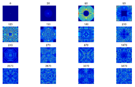
Figure 1: (Color online) Snapshots of the field evolution in the cavity for various $t$.

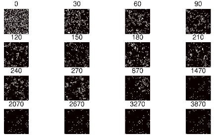
Figure 2: (Color online) Snapshots of the CA evolution in the cavity for various $t$ at $J=1$ ($T=10$).

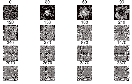
Figure 3: (Color online) Snapshots of the CA evolution in the cavity for various $t$ at $J=5$ ($T=10$).

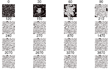
Figure 4: (Color online) Snapshots of the CA evolution in the cavity for various $t$ at $J=50$ ($T=10$).

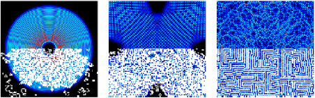
Figure 5: (Color online) Photosensitive cellular automata. Electromagnetic field distribution in the square cavity at different time instants (from left to right, $t=550,1210,33000$). The contemporary CA distribution (a small white box for each LC) is superimposed to the field, only its bottom-half is shown. (parameters $T=0.1$, $J=1100$)

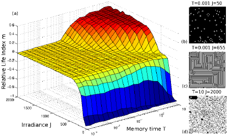
Figure 6: (Color online) Relative Life Index Vs irradiance and memory. The panels on the right show three long-time ($t=4000$) CA configurations with the corresponding parameters.

4 Stationary properties of the CA

The various CA phases can be characterized by the number of LC; this is quantified by the relative life index (RLI) $m$, which is calculated by assigning an Ising spin $\sigma$ with value “-1” to 0 and a “+1” to 1.

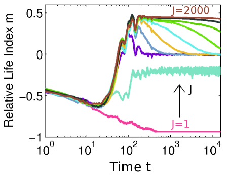
Figure 7: (Color online) Life index Vs time for increasing irradiance (here $T=1$).

The RLI is the average value of $\sigma$ over all the CA. A configuration with many 0s exhibits negative values of $m$ ($m=-1$ for all 0), while $m=1$ for all LC. In the 3D plot of $m$ Vs $T$ and $J$, three regions can be identified (Fig.6a). At very low irradiance (small efficiency or low EM intensity) the final population is organized as in the standard GOL (Fig.6b): it is characterized by small-size unconnected communities of LC (blind phase). Two additional regimes are found while increasing $J$: (i) a glassy phase (where $m=0$) with regular domains separated by various defects (Fig.6c); (ii) a region where the CA is frozen in a large disordered configuration with $m>0$ (Fig.6d). In the glassy phase (plateau in Fig.6a), the CA is not sensible to any increase of $J$. In this regime the EM field sustains a large amount of LC, but their number is frustrated by the internal self-organization. This is true as far as the region with $m>0$ is entered, where an explosive growth of the LC with the irradiance (and the memory time) is found; this is the evolved phase. The existence of this transition is a result of the competition between the GOL rules and the effective employment of the EM energy for life-sustenance.

5 Dynamics

In figure 7 we show the time evolution of $m$ for increasing $J$ at a fixed memory. Starting from the same random CA, different histories are determined by EM field. In the blind phase, the CA rapidly evolve to a small number of LC separated in isolated communities (see WolframRMP ). At sufficiently high fluence, the RLI overshoots and then decays to zero. This implies that the EM field favors the life of a large number of CA; however this is sustainable for long times only at very high irradiance (evolved phase); in the other regimes the population steadily decays to $m=0$.

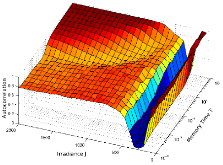
Figure 8: (Color online) Autocorrelation at $\tau=4000$.

Figure 8 shows the autocorrelation function averaged over all the CA:

$$\phi(\tau)=\langle\int\sigma_{i}(t+\tau)\sigma_{i}(t)dt\rangle_{CA},$$ (4)

which is normalized such that $\phi(0)=1$. When increasing the strength of the interaction with the EM field from the blind GOL ($J\cong 0$), the CA first display a disordered dynamical phase ($m\cong-1$ and $\phi\cong 0$), then a glassy region (where $m=0$ and $\phi\cong 0.8$). In the evolved phase ($m\cong 1$), $\phi\cong 1$ denotes a frozen configuration.

6 Self-healing after a catastrophic event

We then consider the reaction of the photosensitive CA to “catastrophic events”. We let the system evolve to a stationary state and then we “kill” all the cells occupying a square in the middle of the box and with size $L/2$ (see figure 9). In the blind phase the system does not react to this event, and the RLI is reduced. Conversely, in the glassy and in the evolved phases, the system rapidly restores the number of LC; at high fluences this is also accompanied by an overshoot of the RLI, which decays to zero in the glassy phase.

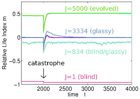
Figure 9: (Color online) Self-healing after a catastrophic event. Relative life index Vs time for various irradiances $J$ (not all values of $J$ for the reported lines are shown) in the presence of the abrupt killing of the living cells in the middle area of the box (at $t=2000$, here $T=1$).

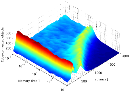
Figure 10: (Color online) Number of edge-connected regions Vs memory time and irradiance.

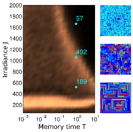
Figure 11: (Color online) Colormap of the number of edge-connected regions; the three dots correspond to the CA panels on the right; connected regions are discriminated by different colors.

7 Topology and self-organization

To characterize self-organization we count the number of edge-connected objects (or communities) in the large time ($t=4000$) CA configuration . Figure 10 shows a three-dimensional plot of the number of edge-connected regions versus the irradiance and the memory time. In the blind phase, one has a large number of unconnected very-small communities with $m\cong-1$. In the glassy phase, many connected regions with $m=0$ are found. In the evolved phase ($m>0$), the CA is organized into a small number of large communities. Specific transition regions can be identified (peaks in Fig.10, brighter lines in Fig. 11) and these are characterized by tiny ranges of the parameters with a huge number of small unconnected communities. Indeed, the transition from the glassy phase to the evolved one is driven by the breaking of the almost regular domains (see panels in Fig.11). Correspondingly the number of communities first increases (in Fig.11 they change from $189$ to $492$) and then rapidly decreases in correspondence to the formation a large amorphous but connected CA at high irradiance.

8 Introducing a genetic code and inheritance

One can argue if the photoreception ability can favor some evolution of the CA toward novel species. The simplest mechanism to be considered is that based on natural selection, such that one assume that a “gene” responsible for photoreception is randomly distributed among the LC. Those LC not displaying such a gene are blind (they obey to the simple GOL rules); the others behave as described above and feel the presence of the EM field. When a new LC is born from the three neighbors [GOL rule (iii) above], it inherits the photoreceptive gene if this is present in two or three of the parents, otherwise it is blind. We find that, as far as no EM field is present, the photosensitive population balances the blind one. When the EM field is introduced, the PLC rapidly supersede the BLC. Figure 12b shows the large-time state of the CA when starting from a balanced configuration (Fig. 12a). Letting $n_{p}$ the number of PLC, and $n_{b}$ that of the BLC, we show the ratio $g=(n_{p}-n_{b})/(n_{p}+n_{b})$ in Fig.13 (left axis) Vs time. In the transparent case, $g$ rapidly reaches the unity.

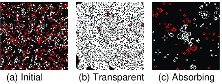
Figure 12: (Color online) Photosensitive CA with genetic code. (a) Initial configuration with same number of blind (red, darker) and photosensitive (white) LC; (b) final configuration for the transparent CA; (c) as in (b) for the absorbing CA ($T=0.1$, $J=50$, $t=1000$).

9 Energy dissipating CA

The “gene” selection process implies that PLC are favored in the presence of an external EM field. The situation however is different if one takes into account the fact that the PLC absorb energy: as their number grows the life-sustaining field is reduced and the selection process is frustrated. In figure 12 we compare the transparent case with the absorbing one ($\sigma=10^{5}$ S m^-1 for the CA material). In the presence of dissipation the fraction of photosensitive agents is reduced, however, surprisingly enough, it stays constant with time after an initial build-up transient.
When considering the snapshots of the EM profile during the CA evolution, one readily realizes that, at variance with transparent case (where the EM wave is de-localized in the entire cavity, see Fig. 5), the field displays a certain degree of localization. Indeed regions with high intensities appears, circumvented by various LC (insets in Fig.13). The effect can be quantified by calculating the EM localization length $l_{EM}$ (see, e.g., Gentilini09 ), reported in Fig.13 (right axis). Notably, after a transient over which the field fills the cavity (up to $t\cong 250$), $l_{EM}$ starts to decrease with time, while $g$ stays constant. As the PLC dissipate energy, the CA is able to localize light (insets in Fig. 13) in order to preserve the intensity level.

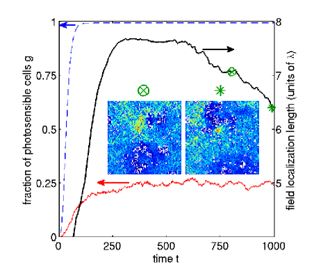
Figure 13: (Color online) Left scale: fraction of PLC Vs time averaged over $100$ initial balanced random condition for transparent (dashed) and absorbing (full line) CA. Right scale: field localization length Vs time ($100$ initial random configuration) for the absorbing CA. The insets show the EM field distributions (for the absorbing case with the CA superimposed) at two instants ($\otimes$ and $\ast$) unveiling the self-organized dynamic wave localization ($J=50$, $T=1$).

10 Conclusion

Within the proposed model of photosensitive (artificial) life, one finds that the development of photoreception largely affects not only the number of living automata but also their organization. If the storage time is too small, the population cannot grow; it wastes energy more quickly than the time needed to collect it. Conversely, an explosive growth is found at the expense of large-scale self-organization, which appears only after a critical degree of photosensibility has been developed. Self-healing abilities after catastrophic events and dynamical hierarchies are triggered by the EM radiation.

When introducing a genetic-like competition between photosensitive and blind CA, the former are favored by the irradiation. If the CA energy dissipation is included, the highly nonlinear EM-CA system results into a self-organized field localization effect, such that the EM localization length decreases with time in order to keep constant the number of photosensitive agents.

The proposed model shows that the competition between the internal rules of a complex system and the development of new abilities (as vision) nurtures abrupt evolutive steps and collective behavior.

11 Acknowledgments

We acknowledge support from the INFM-CINECA initiative for parallel computing. The research leading to these results has received funding from the European Research Council under the European Community s Seventh Framework Program (FP7/2007- 2013)/ERC grant agreement n.201766.

References

- (1) O. Levy, L. Appelbaum, W. Leggat, Y. Gothlif, D. C. Hayward, and D. J. Miller, Science 318, 467 (2007).
- (2) A. Parker, In the blink of an eye (Simon and Schuster, London, 2003).
- (3) S. J. Gould, Wordeful Life: The Burgess Shale and the Nature of History (W. W. Norton, New York, 1991).
- (4) J. McCann, F. Dietrich, and C. Rafferty, Mutat.Res. 411, 45 (1998).
- (5) D. Braun and A. Libchaber, Phys. Rev. Lett. 89, 188103 (2002).
- (6) S. Camazine, J.-L. Deneuborg, N. R. Franks, J. Sneyd, G. Theraulaz, and E. Bonabeau, Self-organization in biological systems (Princeton University Press, 2001).
- (7) A. Yethiraj and A. van Blaaderen, Nature 421, 513 (2003).
- (8) S. Lumsdon, E. Kaler, and O. Velev, Langmuir 20, 2108 (2004).
- (9) S. Duhr and D. Braun, App.Phys.Lett. 86, 131921 (2005).
- (10) P. Reece, E. Wright, and K. Dholakia, Phys.Rev.Lett. 98, 203902 (2007).
- (11) C. Conti, G. Ruocco, and S. Trillo, Phys.Rev.Lett. 95, 183902 (2005).
- (12) D. R. E. Snoswell, C. L. Bower, P. Ivanov, M. J. Cryan, J. G. Rarity, and B. Vincent, New Journal of Physics 8, 267 (2006).
- (13) B. de Lacy Costello, R. Toth, C. Stone, A. Adamatzky, and L. Bull, Phys.Rev. E 79, 026114 (2009).
- (14) I. Sendiña Nadal, E. Mihaliuk, J. Wang, V. Pérez-Muñuzuri, and K. Showalter, Phys. Rev. Lett. 86, 1646 (2001).
- (15) M. A. Bedau, TRENDS Cogn.Sci. 7, 505 (2003).
- (16) M. Gardner, Sci. Am. 223, 120 (1970).
- (17) S. Wolfram, Rev.Mod.Phys. 55, 601 (1983).
- (18) A. Taflove and S. C. Hagness, Computational Electrodynamics: the finite-difference time-domain method (Artech House, London, 2000), 3rd ed.
- (19) S. Gentilini, A. Fratalocchi, A. Angelani, G. Ruocco, and C. Conti, Opt.Lett. 34, 130 (2009).