Prudent walks and polygons

Abstract

We have produced extended series for two-dimensional prudent polygons, based on a transfer matrix algorithm of complexity O$(n^{5}),$ for a series of length $n.$ We have extended the definition to three dimensions and produced series expansions for both prudent walks and polygons in three dimensions. For prudent polygons in two dimensions we find the growth constant to be smaller than that for the corresponding walks, and by considering three distinct classes of polygons, we find that the growth constant for polygons varies with class, while for walks it does not. We give the critical exponent for both walks and polygons. In the three-dimensional case we estimate the growth constant for both walks and polygons and also estimate the usual critical exponents $\gamma,$ $\nu$ and $\alpha.$

1 Introduction

A well-known long standing problem in combinatorics and statistical mechanics is to find the generating function for self-avoiding polygons (or walks) on a two-dimensional lattice, enumerated by perimeter. Recently, we have gained a greater understanding of the difficulty of this problem, as Rechnitzer [1] has proved that the (anisotropic) generating function for square lattice self-avoiding polygons is not differentiably finite [2], confirming a result that had been previously conjectured on numerical grounds [3]. That is to say, the generating function cannot be expressed as the solution of an ordinary differential equation with polynomial coefficients. There are many simplifications of the self-avoiding walk or polygon problem that are solvable [4], but all the simpler models impose an effective directedness or equivalent constraint that reduces the problem, in essence, to a one-dimensional problem.

Prudent walks were introduced to the mathematics community by Préa in an unpublished manuscript [5] and more recently reintroduced by Duchi [6]. A prudent walk is a connected path on ${\mathbb{Z}}^{2}$ such that, at each step, the extension of that step along its current trajectory will never intersect any previously occupied vertex. Such walks are clearly self-avoiding. We take the empty walk, given by the vertex $(0,0)$ to be a prudent walk. Fig. 1 shows a typical prudent walk of $n=2000$ steps, generated via Monte Carlo simulation using a pivot algorithm. Note the roughly linear behaviour – it is believed, although unproven, that the mean-square end-to-end distance grows like $n^{2}$ for prudent walks, i.e. that $\nu=1$.

Figure 1: Typical prudent walk of $n=2000$ steps, generated via Monte Carlo simulation using a pivot algorithm.

The bounding box of a prudent walk is the minimal rectangle containing the walk. The bounding box may reduce to a line or even to a point in the case of the empty walk. One significant feature of two-dimensional prudent walks is that the end-point of a prudent walk is always on the boundary of the bounding box. Each step either lies along the boundary perimeter, or extends the bounding box. Note that this is not a bijection. There are walks such that each step lies on the perimeter of the bounding box that are not prudent. Such walks we call perimeter walks, and they will be the subject of a future publication [7]. Furthermore, if one extends the definition of prudent walks to three-dimensional walks, then it is not true that each step of the walk lies on the perimeter of the bounding box. Again, one can define three-dimensional walks with the property that each step lies on the perimeter of the bounding box, and these too will be discussed in the aforementioned publication [7].

Another feature of prudent walks that should be borne in mind is that they are, generally speaking, not reversible. If a path from the origin to the end-point defines a prudent walk, it is unlikely that the path from the end-point to the origin will also be a prudent walk. Ordinary SAW are of course reversible.

A related, but not identical, model was proposed more than twenty years ago in the physics literature [8], where it was named the self-directed walk. In [8] the authors conducted a Monte Carlo study and found that $\nu=1$, where $\langle R^{2}\rangle_{n}\sim cn^{2\nu}$. Here $\langle R^{2}\rangle_{n}$ is the mean square end-to-end distance of a walk of length $n$. They also sketched an argument that the critical exponent $\gamma,$ characterising the divergence of the walk generating function, $C(x)=\sum c_{n}x^{n}\sim A(1-\mu x)^{-\gamma}$ should be exactly 1, corresponding to a simple pole singularity. This model differs from prudent walks in that different probabilities are assigned to different walks, depending on the number of allowable choices that can be made at each step. For the problem of prudent walks, all realisations of $n$-step walks are taken to be equally likely.

The problem proposed by Préa was subsequently revived by Duchi [6] who also studied two proper subsets, called prudent walks of the first type and prudent walks of the second type (see figure 2 for examples). Prudent walks of the first type are prudent walks in which it is forbidden for a west step to be followed by a south step, or a south step to be followed by a west step. Equivalently, prudent walks of the first type must end on the northern or eastern sides of the bounding box. Such walks are sometimes referred to as 2-sided prudent walks.

Figure 2: Typical examples of: $a)$ a type 1 prudent walk, $b)$ a type 2 prudent walk, $c)$ a general prudent walk, and $d)$ a prudent polygon.

Prudent walks of the second type are prudent walks in which it is forbidden for a west step to be followed by a south step when the walk visits the top of its bounding box and a west step followed by a north step when the walk visits the bottom of its bounding box. Equivalently, prudent walks of the second type must end on the northern, eastern or southern sides of their bounding box. Such walks are sometimes referred to as 3-sided prudent walks. Duchi found the solution for prudent walks of the first type, and gave functional equations for the generating function of (unrestricted) prudent walks. More recently the problem has been revisited by Bousquet-Mélou [9], who gave a systematic treatment of all three types, and in particular gave the solution for the generating function for prudent walks of the second type.

Results for prudent walks (unrestricted) can be found in [10].

2 Computer enumeration

In two dimensions, we use transfer-matrix algorithms to count the number of prudent walks and polygons. Given a prudent walk, only a small amount of information about the walk is required in order to determine how to extend the walk by a single step so as to form a longer prudent walk. This information is called a configuration. Any prudent walk of a given length corresponds to a unique configuration and there is only a finite number of configurations. Our algorithm progresses by computing the number of walks of length $m$ corresponding to each possible configuration and then adding a single step at a time to each configuration, that is adding a step to each walk in the equivalence class of walks corresponding to a given configuration. This is repeated (starting from a walk of size 1) until a given maximal length $n$ is reached. The information that needs to be stored in a configuration depends on which sub-class of prudent walks or polygons we are counting.

Consider unrestricted prudent walks. Any partial walk of say $m$ steps will be contained within a bounding box, which is the smallest rectangle into which we can fit the walk. It is easy to show that the end-point of the walk must be on a side of this box. The next step must either move away from the box, making it larger, or along the current side, which is possible only if the walk has not already visited vertices lying in that direction.

The information needed to describe the configuration of prudent walks is the dimensions of the bounding box, which side of the box the walk end-point is on, the location of the end-point on that side, and an integer representing the directions in which the walk is allowed to be extended, i.e. whether there are sites of the walk along the side to the left of the end, to the right of the end, or neither (both is not possible.)

Without loss of generality, we can assume that the end-point of the walk is on the top side of the bounding box, since direction is not important for unrestricted prudent walks. We can also assume that the end of the walk is not farther from the left side than from the right side, since the number of ways in which a walk can be completed is invariant under reflection.

For a given configuration, there are three possible steps a walk can take:

• A step outward, away from the current side;

• A step to the left along the current side, if there are no walk sites in that direction;

• A step to the right along the current side, if there are no walk sites in that direction.

When we move from a side to a corner of the bounding box, we consider the end-point of the walk to have moved to the other side only if that side has been moved outward by the step.

The transfer-matrix algorithm proceeds by adding a single walk step at a time. We keep a list of the possible configurations and the number of walks in the equivalence class of that configuration. The algorithm steps through the list, and for each source configuration $s$, generates the new target configurations $t_{j}$ that can be obtained by adding a single step (there are at most three new target configuration $t_{j}$ per source configuration). We then add the number of walks $c_{s}$ with the source configuration $s$ to the number of walks $c_{t_{j}}$ of each of the target configurations $t_{j}$. The length of a walk is equal to the number of iterations of the algorithm and the total number of walks of a given length is found by summing the number of walks $c_{s}$ in the list of source configurations.

For prudent polygons, the position of the end-point of the walk is not enough information to determine if the walk can be extended to create a prudent polygon. The position of the start-point of the walk is also required. So we have to extend a configuration to include the coordinates of the start-point of the walk.

If the start of the walk is not on one of the sides of the bounding box, nor adjacent to a site on the current bounding box side that is in a direction in which the walk can extend, then the walk cannot be extended to form a prudent polygon, and we do not need to calculate the number of walks with that configuration. So if such a configuration is generated by the transfer matrix algorithm, it is discarded.

If we are enumerating polygons of size $n$, and for a given configuration of $m$-step walks we cannot reach a site adjacent to the end point in $n-m$ steps or less, then we can ignore that configuration.

When calculating the number of polygons of a given size, we sum the number of walks only for those configurations $s$ where the end-point is adjacent to the start-point.

The number of configurations grows like $n^{4}$. The width $w$ of the bounding box can vary from 1 to $n$ while the length $l$ can vary from 1 to $n-w$. Some smaller boxes cannot occur because for $w\times l<n$ the walk cannot fit within the box, but we shall ignore this effect for simplicity. In a box of size $w\times l$ the end-point can be in any of the $w$ positions on the top edge while the starting point can be in $3w+2l$ positions, so up to constant factors (arising from the restrictions on the directions the walk may take etc.) we have that the number of configuration must be proportional to

$$\sum_{w=1}^{n}\sum_{l=1}^{n-w}w(3w+2l)<\sum_{w=1}^{n}\sum_{l=1}^{n}w(3w+2l)<\sum_{w=1}^{n}(3w^{2}n+2wn^{2})={\rm O}(n^{4})$$

As indicated above we do not have to keep all configurations but can discard some because they won’t give a prudent polygon of size $\leq n$. This however does not help reduce the asymptotic growth in the number of configurations which remains at ${\rm O}(n^{4})$ and the computational complexity of the algorithm is thus ${\rm O}(n^{5})$.

In prudent walks and polygons of types 1 and 2, we cannot ignore the direction of the current edge in our configuration, since some steps may be disallowed depending on their direction. So we cannot assume that the end-point is on the top edge, or arbitrarily reflect the configuration, since rotations and reflections of a configuration are not equivalent. However, for type 1 walks and polygons we can reflect about the southwest-to-northeast axis; and for type 2 walks we can reflect about the east-west axis.

Apart from the precise information required in the configuration, the test for which steps are valid from a given configuration, and which configurations should be accumulated to give the result, the algorithm to enumerate each of these six objects (type 1, type 2 and full walks and polygons) is identical. So we produced one program to solve all of these problems. The lists are stored in hash tables for efficiency. The number of walks for each configuration and the total number of walks or polygons are computed modulo a large prime number close to the computer’s word size. The computation is repeated for several primes and the final result is calculated by use of the Chinese remainder theorem. This is more efficient than performing the whole calculation using numbers larger than the computer’s word size.

In the following sections we show that for prudent walks and polygons of types 1 and 2 the generating functions can be derived rigorously or found from relatively short series. The exceptions are unrestricted prudent walks and polygons, and in the former case the number of walks can be calculated efficiently by iteration of a functional equation. So the only case requiring serious computational effort is that of unrestricted prudent polygons. We enumerated the number of prudent polygons up to size 1004. The calculation was performed on the SGI Altix cluster of the Australian Partnership for Advanced Computing (APAC). This cluster has a total of 1920 1.6GHz Itanium2 processors.

The algorithm was parallelised in a fairly straightforward manner with configurations distributed across processors using a basic hashing scheme. As in the basic algorithm, we step through the list of source configurations and generate all the new target configurations. For each target we check, using our hashing scheme, on which processor the target should reside. If this is not the current processor the configuration and its count is stored in a temporary stack. At regular intervals we pause in the main calculation in order to distribute the configurations from the temporary stacks to their designated processors. We found experimentally that it was advantageous to do the ‘parallel’ hashing using only the bounding box and starting-point information from the configuration. Also doing the updating of the walk counts is fairly cheap and for this reason we did several primes simultaneously in a single run. To reproduce the integer coefficients correctly up to 1004 steps required some 36 primes so in practice we did 4 runs with each run using 9 primes. Each run utilised 160 processors and took about 9 hours with about 1/3 of this time used in the communications part of the algorithm. In total we used some 5500 CPU hours.

3 Prudent walks

In this section we summarise the known results for prudent walks. More detail can be found in [9, 10]. We denote the generating function of prudent walks of the first type by

$$C^{(1)}(x)=\sum c^{(1)}_{n}x^{n},$$

where $c^{(1)}_{n}$ is the number of $n$-step prudent walks of the first type. Then [6]

$$C^{(1)}(x)=1+x\frac{(1-2x-x^{2})(3+2x-3x^{2})+(1-x)\sqrt{(1-x^{4})(1-2x-x^{2})}}{(1-2x-x^{2})(1-2x-2x^{2}+2x^{3})}.$$ (1)

It is clear that the dominant singularity is a simple pole located at the real positive zero of the polynomial $1-2x-2x^{2}+2x^{3},$ notably at $x=x_{c}=0.4030317168\ldots.$ Thus the critical exponent $\gamma=1,$ and the asymptotic form of the coefficients is

$$c_{n}^{(1)}=\lambda^{(1)}/x_{c}^{n}+{\rm o}(\rho^{-n}),$$

for any $\rho<\sqrt{2}-1,$ where $\lambda^{(1)}=\frac{x_{c}(3x_{c}-1)}{(3x_{c}+1)(5x_{c}-2)}\approx 2.5165\ldots.$

We denote the generating function of prudent walks of the second type by

$$C^{(2)}(x)=\sum c^{(2)}_{n}x^{n}$$

where $c^{(2)}_{n}$ is the number of $n$-step prudent walks of the second type.

The generating function, first found by Bousquet-Mélou [9] is much more complicated than that for prudent walks of the first type. First, we define

$$q\equiv q(x)=\frac{1-x+x^{2}+x^{3}-\sqrt{(1-x^{4})(1-2x-x^{2})}}{2x}.$$ (2)

Then

$$C^{(2)}(x)=\frac{1}{1-2x-x^{2}}\left(2x^{2}qT(x;1)+\frac{(1+x)(2-x-x^{2}q)}{1-xq}\right)-\frac{1}{1-x},$$

where

$$T(x)\equiv T(x;w)=\sum_{k\geq 0}(-1)^{k}\frac{\prod_{i=0}^{k-1}(\frac{x}{1-xq}-U(q^{i+1}))}{\prod_{i=0}^{k}(\frac{xq}{q-x}-U(q^{i}))}\left(1+\frac{U(q^{k})-x}{x(1-xU(q^{k}))}+\frac{U(q^{k+1})-x}{x(1-xU(q^{k+1}))}\right),$$ (3)

and

$$U(w)\equiv U(x;w)=\frac{1-wx+x^{2}+wx^{3}-\sqrt{(1-x^{2})(1+x-wx+wx^{2})(1-x-wx-wx^{2})}}{2x}.$$

In this case the asymptotics are much more difficult to establish. Bousquet-Mélou [9] has confirmed that the dominant singularity is precisely as for type 1 prudent walks, that is to say, a simple pole located at the real positive zero of the polynomial $1-2x-2x^{2}+2x^{3},$ notably at $x=x_{c}^{(1)}=0.4030317168\ldots.$ The factor

$$\prod_{i=0}^{k}(\frac{xq}{q-x}-U(q^{i}))$$

appearing in the denominator of (3) gives rise to an infinite sequence of poles on the real axis, lying between $x_{c}$ and $\sqrt{2}-1,$ which are not canceled by zeros of the numerator. This accumulation of poles is enough to prove that the generating function cannot be D-finite.

Prudent walks have no additional geometric restrictions, the only restriction being that they are prudent. We denote the generating function of such walks as

$$C(x)=\sum c_{n}x^{n},$$

where $c_{n}$ is the number of $n$-step prudent walks. Duchi gave two coupled equations which can be iterated to give the series coefficients of prudent walks in polynomial time. Rechnitzer pointed out that these equations can be combined into a single equation,

$$\frac{1}{xw}H(u,v,w)=1+H(u,v,w)+H(u,v,w)+H(u,v,w)+$$ (4)

$$\frac{xu}{v-xu}(H(u,v,w)-H(u,xu,w))+\frac{xv}{u-xv}(H(u,v,w)-H(v,xv,w)),$$

which can be iterated, and the generating function obtained by setting $u=v=w=1.$ A closed form solution for this problem has not been found. In earlier work [10] the first 400 series coefficients were obtained and analysed, and it was conjectured that the critical point and critical exponent remain unchanged from those of prudent walks of type 1 and type 2. That is to say, type 1, type 2 and unrestricted prudent walks have the same critical point, and the same critical exponent $\gamma=1,$ corresponding to a simple pole.

The anisotropic generating function can be defined as follows: If $c_{m,n}$ denotes the number of prudent walks with $m$ horizontal steps and $n$ vertical steps, then the anisotropic generating function can be written

$$C(x,y)=\sum_{m,n}c_{m,n}x^{m}y^{n}=\sum_{n}R_{n}(x)y^{n},$$

where $R_{n}(x)=\frac{M_{n}(x)}{N_{n}(x)}$ is the (rational [11]) generating function for prudent walks with $n$ vertical steps.

We [10] calculated the first 10 generating functions $R_{1}(x),\ldots,R_{10}(x)$ and found a regular pattern in the denominators $N_{n}(x),$ with factors corresponding to cyclotomic polynomials of steadily increasing degree. If this pattern persists, the generating function cannot be D-finite, as the pattern of cyclotomic polynomials of increasing degree implies a build-up of zeros on the unit circle in the complex $x$ plane, and such an accumulation is incompatible with D-finite functions. As noted above, type-2 prudent walks are not D-finite, and the numerical evidence here allows us to conjecture that (anisotropic) unrestricted prudent walks are also not D-finite.

4 Prudent polygons

Polygon analogues of these three classes of walks can be naturally defined as walks of the given class that end at a vertex adjacent to their starting vertex. The relevant generating functions are

$$P^{(1)}(x)=\sum p^{(1)}_{n}x^{n},$$

where $p^{(1)}_{n}$ is the number of $2n$-step prudent polygons of the first type,

$$P^{(2)}(x)=\sum p^{(2)}_{n}x^{n},$$

where $p^{(2)}_{n}$ is the number of $2n$-step prudent polygons of the second type, and

$$P(x)=\sum p_{n}x^{n},$$

where $p_{n}$ is the number of $2n$-step prudent polygons. See Fig. 2 for an example of a prudent polygon. We have generated extensive isotropic and anisotropic series expansions for prudent polygons.

Just as we did for prudent walks above, if we distinguish between steps in the $x$ and $y$ direction, and let $p_{m,n}$ denote the number of prudent polygons with $2m$ horizontal steps and $2n$ vertical steps, then the anisotropic generating function for polygons can be written

$$P(x,y)=\sum_{m,n}p_{m,n}x^{m}y^{n}=\sum_{n}H_{n}(x)y^{n},$$

where $H_{n}(x)=\frac{R_{n}(x)}{S_{n}(x)}$ is the (rational [11]) generating function for prudent polygons with $2n$ vertical steps.

4.1 Type-1, or 2-sided prudent polygons.

We generated more than 100 terms of the series for type 1 polygons, as described in the previous section, which was more than sufficient to identify the generating function.

For prudent walks of the first type, we found, experimentally, that the generating function satisfies a second order linear ODE,

$$\sum_{i=0}^{2}P_{i}(x)f^{(i)}(x)=0,$$

where

$$P_{0}(x)=(-18+72x-99x^{2}+42x^{3}-30x^{4}+32x^{5}-7x^{6}+2x^{7}),$$

$$P_{1}(x)=(1-x)(-12+78x-148x^{2}+97x^{3}-39x^{4}+47x^{5}-9x^{6}+4x^{7}),$$

$$P_{2}(x)=x(1-x)^{2}(1-3x-x^{2}-x^{3})(3-7x+2x^{2}-x^{3}),$$

which can be solved to yield

$$xP^{(1)}(x)=\sum p_{n}^{(1)}x^{n+1}=\frac{(1-3x+x^{2}+3x^{3})}{(1-x)}-\sqrt{(1-x)(1-3x-x^{2}-x^{3})}.$$ (5)

This result has recently been proved by Schwerdtfeger [12], who showed it can be derived from the known result for the generating function of bar-graph polygons, as type-1 prudent polygons are essentially bar-graph polygons. From (5) it can be seen that

$$p^{(1)}_{n}=const.\mu_{1}^{2n}\times n^{-3/2}(1+{\rm O}(1/n)),$$

where $1/\mu_{1}^{2}$ is the smallest positive root of the polynomial $1-3x-x^{2}-x^{3}.$ The smallest root is at $x_{c}=0.29559774\ldots,$ so $\mu_{1}=1.8392867\ldots.$ This should be compared to $\mu=2.4811943\ldots$ for type-1 prudent walks. Clearly, prudent polygons are exponentially rare among prudent walks, unlike the analogous situation for ordinary SAW, for which it is known that the growth constants of SAW and SAP are the same.

Using the conventional exponent notation, so that $P^{(1)}(x)\sim const.(1-\mu_{1}^{2}x)^{2-\alpha},$ we see that $\alpha=3/2.$

4.2 Type-2, or 3-sided prudent polygons.

For prudent polygons of the second type, we again generated long series, but were unable to find the generating function by numerical experimentation. Given the complexity of the known generating function for type-2 prudent walks, this is perhaps not surprising. Nevertheless, we were able to obtain quite precise numerical results, allowing us to conjecture

$$P^{(2)}(x)\sim const.(1-\mu_{2}^{2}x)^{2-\alpha},$$

where, again, $\alpha=3/2.$ However, for $\mu_{2}$ we find $\mu_{2}=2.023896\ldots,$ which is greater than $\mu_{1}$ and shows that type-1 prudent polygons are exponentially rare among type-2 prudent polygons, which are in turn exponentially rare among type-2 prudent walks.

Very recently Schwertdfeger [12] has obtained the exact generating function for these polygons, incidentally confirming our numerical conjectures. He finds the generating function to be

$$P^{(2)}(x)=2\left(\frac{x^{2}}{1-x}+B(x,1)+R(x)\right)$$

where

$$B(x,u)=\frac{1-x-u(1+x)x-\sqrt{x^{2}(1-x)^{2}u^{2}-2x(1-x^{2})u+(1-x)^{2}}}{2xu}$$

and

$$R(x)=\sum_{k\geq 0}L((xq^{2})^{k})\prod_{j=0}^{k-1}K((xq^{2})^{k}),$$

where

$$q=\frac{1+x^{2}-\sqrt{1-4x+2x^{2}+x^{4}}}{2x},$$

$$L(x)=\frac{(1+x^{2}-(1-2x+2x^{2}+x^{4})q)(B(x,q)+x)}{1-x(1+x)q-(x(1-x-x^{3})q+x^{2})(B(x,q)+x)}$$

and

$$K(x)=\frac{(1-x)q-1-((1-x+x^{2})q-1)(B(x,q)+x)}{1-x(1+x)q-(x(1-x-x^{3})q+x^{2})(B(x,q)+x)}.$$

Asymptotic analysis of this expression [12] shows that the dominant singularity is given by the real positive zero of $x^{5}+2x^{2}+3x-2,$ which occurs at $x=x_{c}=0.49409642\ldots=1/2.0238964\ldots,$ and the singularity of the generating function is a square-root singularity, just as for type 1 prudent polygons. Both the location of the singularity and its exponent confirm our earlier numerical work.

Turning to the anisotropic generating function, we find numerically that

$$H_{n}=\frac{x^{n+1}P_{n}(x)}{(1-x^{2})^{n}},$$

for $n$ even, and

$$H_{n}=\frac{x^{n+2}P_{2n}(x)}{(1-x^{2})^{n}}$$

for $n$ odd. This denominator behaviour is not inconsistent with a D-finite generating function, but is precisely of the form observed for type-2 prudent walks, which are not D-finite. It is therefore not surprising that the generating function for the isotropic type 2 polygon is not D-finite, though the functional form of the anisotropic generating function above gives no clue as to this fact. However, this result has been confirmed, in the isotropic case, by Schwertdfeger [12], who proved non D-finiteness.

4.3 Unrestricted, or 4-sided prudent polygons.

Again we resorted to a numerical study. The methods we used to analyse and estimate the asymptotic behaviour of the series have all been described in [13]. We found from our analysis that the series expansion is quite badly behaved, with evidence of very strong sub-dominant asymptotic behaviour that mask the dominant asymptotic behaviour until quite large values of $n$ are reached. Our initial attempts at a differential approximant analysis were not as convincing as they usually are. This was not really surprising, as there is evidence of a large number of singularities on the real axis, just beyond the critical point. This is the known situation for type-2 polygons, where there is an infinite number of poles in a small range of the real axis, just beyond the critical point. It is unremarkable that unrestricted polygons behave similarly. Nevertheless, using 3rd order inhomogeneous approximants, and a series of 125 coefficients, corresponding to a maximum perimeter of 250, we were able to estimate the critical point at $x_{c}=1/\mu_{P}^{2}=0.2267\pm 0.0004,$ or $\mu_{P}=2.100\pm 0.002.$ The singularities appeared to be double roots, and we could not get a consistent estimate of the exponent.

Accordingly, we based our analysis on ratio type methods, which generally are much more slowly convergent than differential approximant methods, but have the advantage that convergence, when it eventually does take place, is more evident.

Indeed, we had to generate some 500 terms in the series (corresponding to polygons with perimeter of up to 1000 steps), before we could get a reasonably clear picture of the asymptotics, and even then it is not as unequivocal as we would like. To estimate the critical point, we used a range of extrapolation methods to extrapolate the ratio of successive terms. We first used Wynn’s algorithm, which is known to be slowly convergent, but robust. The first iterates of the ratios were monotonically increasing, beyond $4.3987.$ This sequence should converge to $\mu_{P}^{2}.$ The second iterate was also steadily increasing, suggesting that $\mu_{P}^{2}>4.4038.$ Higher iterates were unstable.

We next used Brzezinski’s $\theta$ algorithm, which is known to be rapidly convergent under optimal circumstances. The first iterates of the ratios were monotonically increasing for 84 terms, then decreasing until 187 terms, then increasing again, beyond $4.4155.$ This sequence may continue to exhibit oscillatory behaviour, so we are reluctant to use it as anything other than a guide. The second iterates started oscillating quite early in the sequence. Higher iterates were unstable.

We next used the Levin $u$-transform, which is also known to be rapidly convergent in ideal circumstances. The first iterates of the ratios were monotonically increasing for the first 122 ratios, then steadily decreasing, and seemingly approaching an asymptote at a value of 4.4157. The second iterates reached a minimum at 198 terms, then steadily increased, and also approached an asymptote around 4.4157, though this is of no significance, as the previous iterates were all around that value, so one would expect an iteration of an almost constant sequence to give that constant value. Higher iterates were unstable.

Finally, a Neville table gave monotone first and second iterates. The first iterates were steadily increasing, suggesting $\mu_{P}^{2}>4.4107,$ while the second iterates increased more slowly, and gave $\mu_{P}^{2}>4.4128.$ The third iterates reached a maximum at 116 terms, and then a minimum at 201 terms, and then steadily increased. If this monotone trend continues, we can conclude $\mu_{P}^{2}>4.4136.$ Combining all these methods, we estimate $\mu_{P}^{2}=4.415\pm 0.001$ or $\mu_{P}=2.1012\pm 0.00025$ which encompasses all the results.

In figure 3 we show a plot of the ratios of successive terms plotted against $1/n.$ Assuming the generating function behaves as $P(x)\sim const.(1-\mu_{P}^{2}x)^{2-\alpha},$ then asymptotically, the ratios should approach $\mu_{P}^{2},$ with gradient $\mu_{P}^{2}(\alpha-3).$ From the ratio plot, a limit around 4.415 is very plausible, though there is still a small amount of curvature in the locus of ratios. This is almost certainly due to the presence of exponentially small corrections due to one or more nearby singularities on the real axis. Extrapolating this locus to the estimated limit $\mu_{P}^{2}\approx 4.415,$ we estimate the slope in the vicinity of the $y$-axis to be $-20,$ so that $\alpha\approx-1.5.$ We have also used biased differential approximants, with the critical point biased at $\mu_{P}^{2}=4.415,$ and while this signalled a confluent singularity at the critical point, it gave a consistent value for the exponent, $\alpha-2$ as $-3.5\pm 0.1,$ so that again $\alpha\approx-1.5.$

In summary, we find for the generating function, $P(x)\sim const.(1-\mu_{P}^{2}x)^{2-\alpha},$ where now $\alpha\approx-1.5.$ We do not quote error bars as this estimate of $\alpha$ is very sensitive to the estimate of the critical exponent used to bias the results. If we bias the critical point at $\mu_{P}^{2}=4.416,$ a change of only 1 in the least significant digit, the exponent estimate from differential approximants changes to $-4.2\pm 0.02.$ Thus our estimate of $\alpha$ can only be taken as indicative, rather than precise. What is clear however is that the singularity is unlikely to be of square-root type, as is the case for type 1 and type 2 polygons, but of course there is no obvious reason why it should be.

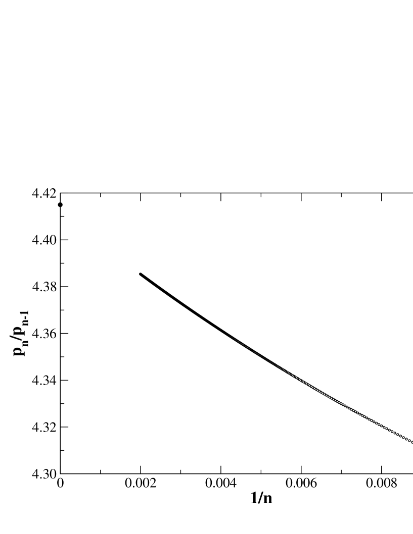
Figure 3: Plot of successive ratios of terms $p_{n}/p_{n-1}$ against $1/n$ for prudent polygons of half-perimeter $n$. Our best estimate for the critical point $\mu_{P}^{2}=4.415$ is marked with a large dot on the $y$-axis.

For the anisotropic case, we write the generating function as

$$P(x,y)=\sum_{m,n}p_{m,n}x^{m}y^{n}=\sum_{n}H_{n}(x)y^{n},$$

where the first few $H_{n}(x)$ are:

$$H_{1}(x)=\frac{1+x-x^{2}}{(1-x)^{3}}$$

$$H_{2}(x)=\frac{1+3x+2x^{2}+x^{3}}{(1-x)^{5}}$$

$$H_{3}(x)=\frac{1+5x+x^{2}-3x^{3}+x^{5}}{(1-x)^{5}(1+x)}$$

$$H_{4}(x)=\frac{1+7x+16x^{2}+18x^{3}+12x^{4}+4x^{5}+x^{6}}{(1-x)^{7}(1+x)}$$

$$H_{5}(x)=\frac{1+11x+19x^{2}+3x^{3}-12x^{4}+5x^{5}+6x^{6}-x^{7}-x^{8}}{(1-x)^{7}(1+x)^{2}}$$

$$H_{6}(x)=\frac{V_{9}(x)}{(1-x)^{9}(1+x)^{2}}$$

$$H_{7}(x)=\frac{V_{14}(x)}{(1-x)^{9}(1+x)^{4}(1+x+x^{2})}$$

$$H_{8}(x)=\frac{V_{15}(x)}{(1-x)^{11}(1+x)^{4}(1+x+x^{2})},$$

where $V_{i}(x)$ denotes a polynomial of degree $i.$ From the above, we see the relentless build-up of cyclotomic polynomials of increasingly high order. As is well-known, if this pattern persists, the underlying generating function cannot be D-finite. While this does not a priori prove that the isotropic generating function is not D-finite, we know of no combinatorial problem where this is the case. That is to say, where the isotropic generating function is D-finite, while the anisotropic generating function is not.

5 Three-dimensional walks and polygons

We have enumerated all prudent walks of up to $n=23$ steps on the three-dimensional simple cubic lattice, using a simple backtracking algorithm. As for the case of ordinary SAW, it is a far more difficult task to perform enumerations in three dimensions than it is in two. To take advantage of the inherent symmetry in the problem we only explicitly counted walks whose first step was in the positive $x$ direction, whose first step out of this line (if any) was in the positive $y$ direction, and whose first step out of this plane (if any) was in the positive $z$ direction. In addition, we trivially parallelized the backtracking algorithm: In three dimensions there are sixteen 4-step prudent walks whose first two steps are precisely East then North. We independently enumerated the completions to $n$-step walks of each of these prefixes. Similarly there are four 4-step prudent walks whose first three steps are East, East, North. Again we independently enumerated the $n$-step completions of each of these prefixes. Finally, the prudent walks whose first three steps are East, East, East were all enumerated together in the same computation. Thus, for each value of $n$ we ran a total of 21 independent computations. The enumerations for $n=23$ took a total of around 2377 hours (roughly 100 hours per independent computation). The computations were performed on tango, a 95-node Linux cluster at the Victorian Partnership for Advanced Computing (VPAC). Each node consists of two AMD Barcelona 2.3GHz quad core processors. In principle, it is probably possible to obtain another term or two by applying the two-step method [14], but we have not pursued this here.

For each $1\leq n\leq 23$ we computed the number of prudent walks, $c_{n}$, the number of prudent polygonal returns, $u_{n+1}$, and the sum of squared end-to-end distances $c_{n}\,\langle R^{2}\rangle_{n}$, summed over all prudent walks. The results of our enumerations are presented in Table 1.

Table 1: Exact enumeration data on the simple cubic lattice. Here $c_{n}$ denotes the number of $n$-step prudent walks, $u_{n+1}$ the number of $(n+1)$-step prudent polygonal returns, and $\langle R^{2}\rangle_{n}$ the average squared end-to-end distance of $n$-step prudent walks.

$n$	$c_{n}$	$c_{n}\,\langle R^{2}\rangle_{n}$	$u_{n+1}$
0	1	0	0
1	6	6	0
2	30	72	0
3	150	582	24
4	726	4032	0
5	3510	25542	240
6	16734	153048	0
7	79518	881118	2544
8	375246	4925616	0
9	1766382	26909934	31800
10	8278638	144356280	0
11	38721366	762839334	435864
12	180556206	3981064368	0
13	840524742	20556000822	6323352
14	3903866526	105173637672	0
15	18106798830	533839505646	95647104
16	83832778110	2690761186608	0
17	387690560718	13478479905486	1493934516
18	1790330065854	67142893855752	0
19	8259528315558	332807521103670	23934001600
20	38059497518214	1642214518277040	0
21	175228328442174	8070246610372494	391427518152
22	805959153119262	39511166688322248	0
23	3704270575724550	192780251992208934	6511949001648

We analysed the various series by the method of differential approximants, as well as variants of the ratio method, as used in the analysis of the polygon generating function in the previous section, (see [13] for a review of these standard methods). For the prudent walk generating function, for which we expect

$$C(x)=\sum c_{n}x^{n}\sim const.(1-x/x_{c})^{-\gamma}$$

we found a singularity on the positive real axis at $x_{c}\approx 0.22265\pm 0.0003$ with corresponding exponent $\gamma=1.68\pm 0.03.$ Biasing the value of the critical point at the central estimate, that is setting $x_{c}=0.22265$ gives the corresponding biased estimate of $\gamma=1.67$ from first order differential approximants, and $\gamma=1.68$ from second-order differential approximants. For SAW, the analogous values are $x_{c}({\rm SAW})\approx 0.2134907$ and $\gamma_{\rm SAW}\approx 1.1567,$ so prudent walks are exponentially rare among SAW, and the two models have different critical exponents.

Additionally, for three-dimensional prudent walks we find that there is a singularity in the generating function $C(x)$ on the negative real axis that appears to be at, or just beyond, $x=-x_{c}.$ For the corresponding self-avoiding walk model, it is known that there is a singularity (the analogue of an anti-ferromagnetic singularity for a magnetic model) exactly at $x=-x_{c}({\rm SAW}),$ but the argument for the location of that singularity in the case of SAW does not translate to prudent walks. The corresponding exponent is, very approximately, the same magnitude as that of the physical singularity, but opposite in sign. That is to say, there appears to be a singularity of the form

$$const.(1+x/x^{*})^{\gamma^{*}},$$

where $x^{*}\geq x_{c}$ and $\gamma^{*}\approx\gamma,$ as well as the physical singularity. For two-dimensional prudent walks, there is also evidence of a singularity on the negative real axis, but located considerably further away from the origin than the physical singularity. That is to say, $x^{*}(2d)>x_{c}(2d).$

To calculate the exponent $\nu$ characterising the mean square end-to-end distance, $\langle R^{2}\rangle_{n}\sim const.n^{2\nu}$ we analysed the series for the sum of the squared end-to-end distances, which diverges at $x_{c}$ with exponent $\gamma+2\nu.$ From a differential approximant analysis we found $x_{c}\approx 0.22265$ with $\gamma+2\nu\approx 3.20,$ so that $\nu\approx 0.76.$ We also analysed the series $\langle R^{2}\rangle_{n}$ directly, and obtained an estimate for $\nu$ consistent with that just quoted, but less precise.

The polygonal returns $u_{n}$ include a factor $2n$, corresponding to $n$ possible starting points and a factor of 2 as the path may be traversed clockwise or anticlockwise. We have analysed the series with coefficients $p_{n}=u_{n}/2n.$ We only have 11 coefficients, which is not really enough for any but the crudest analysis. From a differential approximant analysis, we find the generating function $P(z)=\sum_{n}p_{n}z^{n}$ is singular at $z=z_{c}\approx 0.0499\pm 0.0006,$ with an exponent $2.3\pm 0.5.$ That is to say, $P(z)\approx const.(1-z/z_{c})^{2.3}.$ Note that from our analysis of the corresponding walk series, $x_{c}^{2}=0.04957\pm 0.00014.$ Thus it is entirely possible that $z_{c}=x_{c}^{2}$ for three-dimensional prudent polygons, just like the analogous situation for three-dimensional SAW, but unlike the situation for two-dimensional prudent walks and polygons, for which, as discussed above, prudent polygons are exponentially rare among prudent walks. If it is true that $z_{c}=x_{c}^{2}$ for three-dimensional prudent polygons, then we can carry out a biased analysis in which we fix $z_{c}$ at $x_{c}^{2}.$ In that case we find the exponent is a little higher, at $2.5\pm 0.2.$ In terms of the usual notation for critical points, this exponent is $2-\alpha,$ so that $\alpha=-0.5\pm 0.2$

6 Conclusion

We have defined and analysed series for prudent polygons in both two and three dimensions. In two dimensions, we also discussed two subsets, which are exactly solvable. We found that two dimensional prudent polygons are exponentially rare among prudent walks, unlike the situation for two dimensional SAW. We gave numerical arguments in support of the conjecture that the generating function for two dimensional prudent polygons is not D-finite.

We also derived extensive series for three dimensional prudent walks and polygons. As far as we are aware, this problem has not been studied previously. We have given estimates of the critical point and critical exponents. In terms of the usual notation we found that the growth constant for walks is $\mu\approx 4.491,$ with exponents $\gamma\approx 1.68,$ $\nu\approx 0.76,$ and $\alpha\approx-0.3$ based on an unbiased estimate of the critical point. For SAW $\mu_{\rm SAW}\approx 4.68404$, $\gamma\approx 1.1567,$ $\nu\approx 0.5875$ and $\alpha\approx 0.2375.$ For SAW we have the hyper-scaling relation $d\nu=2-\alpha.$ While there is no a priori reason to expect this hyper-scaling relation to hold for three-dimensional prudent walks, as it is a combinatorial model rather than a statistical mechanical model derived from a Hamiltonian, we nevertheless note that $3\nu\approx 2.28$ while $2-\alpha\approx 2.28.$ The uncertainties in our exponent estimates are too great to attach much significance to this approximate equality, except to flag it as a possibility.

In terms of physical significance, the model of prudent walks, while exponentially rare among SAW in both two and three dimensions, is nevertheless exponentially abundant compared to any other solved or numerically estimated model. Other variants of the model that relax the prudency constraint to some extent are likely to be have growth constants even closer to that of SAW, and these will be the subject of a future publication [7].

References

References

- [1] Rechnitzer A 2003 Haruspicy and anisotropic generating functions Adv. Appl. Math. 30 228–257
- [2] Stanley R P 1980 Differentiably finite power series European J. Combin. 1 175–188
- [3] Guttmann A J and Conway A R 2001 Square lattice self-avoiding walks and polygons Ann. Comb. 5 319–345
- [4] Bousquet-Mélou M 1996 A method for the enumeration of various classes of column-convex polygons Disc. Math. 154 1–25
- [5] Préa P 1997 Exterior self-avoiding walks on the square lattice. Unpublished manuscript.
- [6] Duchi E 2005 On some classes of prudent walks. In FPSAC’05 Taormina, Italy, 2005.
- [7] Garoni T M and Guttmann A J 2008 Perimeter and quasi-prudent self-avoiding walks and polygons (in preparation).
- [8] Turban L and Debierre J.-M 1987 Self-directed walk: a Monte Carlo study in two dimensions J. Phys. A: Math. Gen. 20 679–686
- [9] Bousquet-Mélou M 2008 Families of prudent self-avoiding walks, arXiv hal-00276681
- [10] Dethridge J C and Guttmann A. J 2008 Entropy 10 309-318
- [11] Stanley R P 1999 Enumerative Combinatorics vol. 2 (Cambridge: Cambridge University Press)
- [12] Schwertdfeger U 2008 Exact solution of two classes of prudent polygons, arXiv math.CO 0809.5232
- [13] Guttmann A J (1989) Asymptotic analysis of coefficients in Phase Transitions and Critical Phenomena, eds C Domb and J L Lebowitz, (Academic: London) 13 1-234
- [14] Clisby N, Liang R and Slade G 2007 Self-avoiding walk enumeration via the lace expansion, J. Phys. A: Math. Gen. 40 10973–11017