Some remarks on the geometry of the Standard Map

Abstract.

We define and compute hyperbolic coordinates and associated foliations which provide a new way to describe the geometry of the standard map. We also identify a uniformly hyperbolic region and a complementary “critical” region containing a smooth curve of tangencies between certain canonical “stable” foliations.

1. Introduction and informal statement of results

1.1. The standard map

The Standard Map family is a one-parameter family of maps $f_{k}:\mathbb{T}^{2}\to\mathbb{T}^{2}$ on the 2-torus, with a parameter $k\in\mathbb{R}^{+}$, given by

$$f_{k}\begin{pmatrix}x\\ y\end{pmatrix}=\begin{pmatrix}x+k\sin(2\pi y)\\ x+y+k\sin(2\pi y)\end{pmatrix}\mod 1.$$

This family was introduced independently by Taylor and by Chirikov [3] in the late 60’s and is related to a variety of problems in many areas of physics, see for example [19, 23, 17] for extensive discussions. For $k=0$ the map reduces to $f_{0}(x,y)=(x+y,y)$ which is completely integrable (see [19] for full definitions) and $\mathbb{T}^{2}$ is foliated by invariant closed curves.

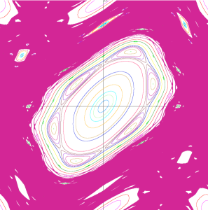
Figure 1. Elliptic islands in a chaotic sea

As $k$ increases these invariant curves break up; the region of parameter values with $k$ small has provided one of the main examples for the application of the KAM theory and its developments such as the studies on the splitting of separatrices [8], formation and properties of Cantori [18] etc., see [6] for a comprehensive review of the theory and and references. Computer pictures show complicated structures in which regions of invariant circles co-exist with apparently more complicated “chaotic” dynamics, see Figure 1. As $k$ increases further these “elliptic islands” shrink until they become essentially invisible and the “chaotic” region seemingly takes over more and more of the phase space. A rigorous description of the structure of the dynamics for large $k$ appears to be an extremely difficult problem.

A basic but still open question is the following.

Question 1.

Are there any values of the parameter $k$ for which $f_{k}$ has positive metric entropy ? Equivalently, are there any values of the parameter $k$ for which $f_{k}$ has an ergodic component of positive measure on which it is (nonuniformly) hyperbolic ?

Numerical evidence suggests a positive answer to this question for large values of $k$ and it seems reasonable to expect the existence of several, possibly infinitely many, ergodic components of positive measure [21] perhaps co-existing with elliptic islands (examples of systems in which these two phenomena are known to co-exist are not many but have been obtained, e.g. in [24]). However, so far the only really rigorous results available point in the opposite direction: there is a dense set of values of $k$ for which the standard map exhibits many elliptic points [7].

It is generally accepted that any progress on this question will require some detailed concrete analysis of the geometry of the standard map, although it is not at all clear from what point of view this geometry should be studied. Some papers have appeared, we just mention [4, 5] in which generating partitions are constructed leading to a symbolic description of the dynamics, and a series of papers by Lazutkin et al [9, 10, 11, 15, 14, 13] suggesting a possible strategy, however a complete implementation of this argument is, to our knowledge, not yet available. We mention also [22] in which a version of the entropy conjecture is proved for some “random approximations” of the standard map. Other families of maps have also been studied which exhibit analogous phenomena as the standard map, see for example the fundamental map introduced in [2].

1.2. Hyperbolic coordinates and approximate critical points

The aim of this paper is to carry out an analysis of certain geometrical features of the standard map which, to our knowledge, have not been investigated before. This analysis is based on the notion of hyperbolic coordinates which essentially consists of carrying out a singular value decomposition of matrix of the derivative $Df_{k}(x)$ at each point $x$, and thus decomposing the tangent space into orthogonal subspaces which are most contracted and most expanded by $Df_{k}(x)$. We shall show (Theorem 1) that this decomposition is well defined at every point $x$ both for $f_{k}$ and well as for its inverse $f_{k}^{-1}$, that it depends smoothly on $x$ and that it defines foliations of the torus $\mathbb{T}^{2}$, see Figure 4. We obtain explicit formulas which allow us to describe the geometry of these foliations in some detail.

The singular value decomposition of a two by two matrix is quite different from the eigenspace decomposition, even in the case of hyperbolic diagonalizable matrices. A first key observation is that the singular value decomposition always yields orthogonal subspaces, whereas this is clearly not necessarily the case for the eigenspace decomposition. A second, non trivial, observation is that in the case of a hyperbolic matrix $A$, the contracting subspaces $e^{(n)}$ of the singular value decomposition of the iterates $A^{n}$ of the matrix, actually converge (exponentially fast) to the contracting eigenspace. It is of course not true that the corresponding expanding subspaces $f^{(n)}$ of the singular value decomposition converge to the expanding eigenspace, since $f^{(n)}$ is always orthogonal to $e^{(n)}$. However, we can consider the inverse $A^{-1}$ of the matrix $A$, for which the contracting and expanding eigenspaces are swapped, and obtain the expanding eigenspace of $A$ which is exactly the contracting eigenspace of $A^{-1}$ as a limit of most contracted directions $e^{(-n)}$ for the singular value decomposition for $A^{(-n)}$.

The notion and properties of hyperbolic coordinates have been systematically developed and applied in [12] for the proof of a version of the Stable Manifold Theorem under quite weak hyperbolicity assumptions and were originally inspired by certain arguments in [1] and [20] on the geometry of Hénon and Hénon-like maps. Indeed, the properties of the convergence of the contracting subspaces apply not only to the iteration of a fixed matrix but also to the composition of different matrices, as occurs naturally, for example, when considering derivatives $Df^{n}(x)$ of higher iterates $f^{n}(x)$ of some map. If the orbit of the not necessarily periodic point $x$ has some hyperbolic decomposition (which generalizes the eigenspace decomposition in the case of a hyperbolic fixed or periodic point), then the contracting directions $e^{(n)}$ converge to the contracting subspace of this decomposition and the contracting directions $e^{(-n)}$ for the inverse map converge to the contracting subspace of the decomposition for the inverse map is exactly the expanding direction for the original map.

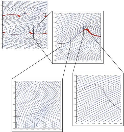
Figure 2. Tangencies between $\mathcal{E}^{(1)}$ and $\mathcal{E}^{(-1)}$.

This approach however really comes into its own when considering points which do not have a hyperbolic decomposition but are points of tangencies between stable and unstable manifolds. Within the framework of hyperbolic coordinates these can be described as points for which the contracting directions $e^{(n)}$ in forward time and the contracting directions $e^{(-n)}$ in backward time both converge but instead of converging to different subspaces, they converge to the same subspace. Indeed, it follows from the properties of stable and unstable manifolds that tangent directions are contracting in forward and backward time respectively. Motivated by these observations we investigate the locus of tangencies between the the most contracting direction $e^{(1)}$ for the standard map $f_{k}$ and the most contracting directions $e^{(-1)}$ for its inverse $f_{k}^{-1}$. We shall show (Theorem 2) that these tangencies occur along two smooth curves, see Figure 2, for which we shall derive explicit expressions which allow us to describe their geometry in considerable detail. These curves are contained in two quite narrow horizontal strips of height of the order of $1/k$. To complement this description we also show (Theorem 3) that $f_{k}$ is uniformly hyperbolic outside these strips.

1.3. General remarks

The study carried out in this paper does not require any very sophisticated arguments or calculations and, in itself, does not yield any spectacular conclusions. It should rather be thought of as a preliminary study of the geometry of the standard map from a novel point of view (though some related foliations to those discussed here appear as part of the arguments in [7]) and with the aim of suggesting certain techniques and directions which might lead to more serious and interesting conclusions.

A full resolution of the so-called “entropy conjecture”, i.e. the existence of parameter values for which the map has positive metric entropy is perhaps still too ambitious a goal, but there are some natural partial results in that direction which seem more feasible. The first one concerns the geometry of such parameters. If the solution to the entropy conjecture is to be achieved through geometric arguments, it would make sense to understand what characteristics the geometry of such a map would have. The state of affairs at the moment is more like trying to prove that a certain phenomenon occurs for some parameter values, but having no idea what we are really looking for or what the geometry of the map would look like at such parameter values. We therefore formulate the following problem.

Question 2.

Construct a geometric model of the standard map with positive entropy.

Models of this kind have been proposed by simplifying the map in certain key aspects. What we mean here however is to describe a model for the occurrence of positive entropy within some member of the actual Standard Map family $f_{k}$ as defined above. Of course such a model would rely on highly non-trivial assumptions about the dynamics, but understanding such a model could lead to an improved understanding of the actual dynamics of the standard map and possibly to a strategy for verifying the assumptions for some parameter values.

One strategy for building such a model would be to start from the geometrical picture described in this paper: two smooth curves of critical points inside two very thin strips and uniform hyperbolicity outside these strips. Considering both forward and backward iterates of the critical strips it should be possible to construct higher order hyperbolic coordinates and thus higher order critical curves, at least in certain parts of the critical strip. Imposing a bounded recurrence condition to the critical strip it may be possible to set up an inductive argument yielding a positive measure set on which the map is nonuniformly hyperbolic and thus has positive metric entropy. Using this strategy it might be possible also to address the following problem which to our knowledge has not been stated before but which would seem to be of independent interest.

Question 3.

Show that for all sufficiently large values of the parameter $k$, any ergodic component of positive measure is (nonuniformly) hyperbolic.

An affirmative answer to this question would reduce the entropy conjecture to showing that for arbitrarily large values of $k$ there are ergodic components of positive measure, though it is not clear that this would simplify the problem.

2. Formal statement of results

The precise statements of our three theorems require a significant amount of notation. We shall therefore state them in three separate section, preceded by the relevant definitions.

2.1. Hyperbolic Coordinates

We start with some general definitions which apply to any surface diffeomorphism $f:M\to M$. For $z\in M$ and $n\geq 1$ let

$$F_{n}(z)=\|(Df^{n}_{z})\|=\max_{\|v\|=1}\{\|Df^{n}_{z}(v)\|\},$$

and

$$E_{n}(z)=\|(Df^{n}_{z})^{-1}\|^{-1}=\|Df^{-n}_{f^{n}(z)}\|^{-1}=\min_{\|v\|=1}\{\|Df^{n}_{z}(v)\|\}.$$

These quantities have a simple geometric interpretation: since $Df_{z}^{n}:T_{z}M\to T_{f(z)}M$ is a linear map, it sends circles to ellipses, see Figure 3,

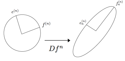
Figure 3. Hyperbolic coordinates of order $n$

then $F_{n}(z)$ is precisely half the length of major axis of this ellipse and $E_{n}(z)$ is precisely half the length of the minor axis of this ellipse. Then let $H_{n}(z)=E_{n}(z)/F_{n}(z).$ Clearly we always have $H_{n}(z)\leq 1$. $H_{n}(z)=1$, or $E_{n}(z)=F_{n}(z)$, means that the image of the unit circle under $Df^{n}$ is itself a circle and $Df^{n}$ is therefore a conformal linear map. On the other hand $H_{n}(z)<1$ is in some sense a (very weak) hyperbolicity condition which implies that the image of the unit circle is strictly an ellipse and that therefore distinct orthogonal unit vectors

$$e^{(n)}(z)\quad\text{ and }\quad f^{(n)}(z)$$

are defined in the most contracted and most expanded directions respectively by $Df^{n}_{z}$. We can use $e^{(n)}(z)$ and $f^{(n)}(z)$ as basis vectors for the tangent space $T_{z}M$ thus can think of them as defining a new system of coordinates which we call hyperbolic coordinates.

The most contracted and most expanded directions, in the open regions in which they are defined, determine direction fields whose regularity is exactly that of the partial derivatives of $f$. Thus, under mild regularity conditions, these open regions admit local integral curves, or foliations, which we denote by

$$\mathcal{E}^{(n)}\quad\text{ and }\quad\mathcal{F}^{(n)}.$$

We can think of the curves of these foliations as finite time stable and unstable manifolds. Indeed, for finite time these curves are more relevant than the real stable and unstable manifolds since they are in some sense the most contracted and most expanded curves under $f^{n}$.

Since $f$ is invertible, all the notions and definitions given above can be applied to $f^{-1}$. We shall talk about hyperbolic coordinates in forward time when referring to the application of these ideas to $f$ and backward time when referring to the application of these ideas to $f^{-1}$.

The first main result of this paper is the detailed description of the geometry of the foliations $\mathcal{E}^{(\pm 1)}$ and $\mathcal{F}^{(\pm 1)}$ for the standard map and its inverse.

Theorem 1.

Contracting foliations $\mathcal{E}^{1},\mathcal{E}^{(-1)}$ and expanding foliations $\mathcal{F}^{(1)},\mathcal{F}^{(-1)}$ are defined everywhere and have the geometry illustrated in the Figure 4 and discussed below.

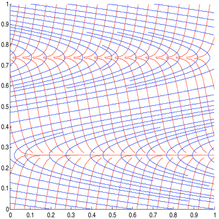
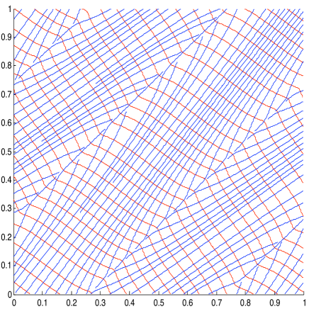
Figure 4. Schematic picture of the stable and unstable foliations ($k=1$) in forward time (left) and backward time (right).

We give here a preliminary discussion of the geometry of these foliations. All statements are formally defined and proved in the following sections.

2.1.1. The contracting foliation in forward time.

The contracting foliation $\mathcal{E}^{(1)}$ consists of essentially horizontal leaves in most of the phase space, although close to the horizontal lines $\{y=1/4\}$ and $\{y=3/4\}$ the leaves exhibit a full horizontal “fold”. The contracting direction $e^{(1)}$ is constant along horizontal lines and thus the tips of the folds lie on a perfectly horizontal line. Figure 4 is drawn for clarity for $k=1$ but in fact for larger $k$ the folds occur in a very thin region. To get an idea, if we define a horizontal strip containing the folds in such a way that the boundaries of the strip are precisely the horizontal lines at which the contracting directions (tangent to the leaves of $\mathcal{E}^{(1)}$) are aligned with the positive and negative diagonals, then the width of this strip is of order $1/k$.

2.1.2. The expanding foliation in forward time

The expanding foliation $\mathcal{F}^{(1)}$ is everywhere orthogonal to $\mathcal{E}^{(1)}$ (since $e^{(n)}$ and $f^{(n)}$ are always orthogonal; a general property of the singular value decomposition). It therefore has exactly two closed leaves given by the horizontal lines through the tips of the folds of the leaves of $\mathcal{E}^{(1)}$. All other leaves wrap around the torus accumulating on these two closed leaves as illustrated in Figure 4. Notice that for large $k$ these leaves are almost vertical moving very “quickly” from one folding region to the other, and then folding very sharply and wrapping infinitely many times round the torus.

2.1.3. The contracting foliation in backward time

This time the contracting direction $e^{(-1)}$ is constant along diagonals, i.e. along lines of slope 1. The foliation $\mathcal{E}^{(-1)}$ has two closed leaves: the two diagonals $\{y-x=1/4\}$ and $\{y-x=3/4\}$. The other leaves of the foliations behave, from a topological point of view, in a similar way to the leaves of the foliation $\mathcal{F}^{(1)}$, each one wrapping infinitely many times around the torus and accumulating on closed leaves. However, from a geometrical point of view, the situation is different. Rather than moving quickly from one closed leaf to the other, the leaves wrap around the torus many times. Moreover, the tangent directions, i.e. the directions of the vectors $e^{(-1)}$ change very rapidly near the closed leaves they , i.e. in a neighbourhood of the closed leaf of width of the order of $1/k$: from an angle of about $\pi/8$ on one side of the closed leaf to an angle of about $3\pi/8$ on the other side of the leaf. Then, more slowly, they essentially re-align themselves with the diagonal in the region between the closed leaves.

2.1.4. The expanding foliation in backward time

As before, the geometry of the expanding foliation $\mathcal{F}^{(-1)}$ is everywhere orthogonal to $\mathcal{E}^{(-1)}$ and is completely determined by the geometry of $\mathcal{E}^{(-1)}$. The general direction of the leaves is along the negative diagonal, exhibiting a peculiar bump as they cross the two closed leaves of $\mathcal{E}^{(-1)}$. This is related to the fact that, as observed in the previous paragraph, hyperbolic coordinates vary very quickly in a neighbourhood of the closed leaves.

2.2. The critical curve of tangencies

We now describe the curve of tangencies between $e^{(1)}$ and $e^{(-1)}$. To obtain an explicit expression for this curve we need to define some constants. First of all we let

$$\delta^{*}:=\frac{1}{2\pi}\cos^{-1}\left(-\frac{1}{4\pi k}\right)\quad\text{ and }\quad\delta^{\pm}:=\frac{1}{2\pi}\cos^{-1}\left(-\frac{1\pm\sqrt{3}}{4\pi k}\right)$$

and

$$\hat{\delta}^{-}_{T}=\frac{1}{2\pi}\cos^{-1}\left(-\frac{1+\frac{\sqrt{3}}{3}}{4\pi k}\right)\quad\text{and}\quad\hat{\delta}^{+}_{T}=\frac{1}{2\pi}\cos^{-1}\left(-\frac{1+3\sqrt{3}}{4\pi k}\right)$$

Notice that

$$1+3\sqrt{3}>1+\sqrt{3}>1+\sqrt{3}/3>1>0>1-\sqrt{3}$$

and therefore, for $k$ large and since the cosine function is decreasing near $\pi/2$ we have

$$\delta^{-}<1/4<\delta^{*}<\hat{\delta}^{-}_{T}<\delta^{+}<\hat{\delta}^{+}_{T}$$

and all five constants tend to $1/4$ as $k\to\infty$. Now let

$$\hat{\Delta}_{T}=[\hat{\delta}^{-}_{T},\hat{\delta}^{+}_{T}]\cup[1-\hat{\delta}^{+}_{T},1-\hat{\delta}^{-}_{T}]$$

denote the union of two horizontal strips defined by the above constants. It will be useful to introduce an alternative coordinate system by writing

$$\tilde{y}=y-x\mod 1.$$

Geometrically, lines of the form $\{\tilde{y}=c\}$ are lines of constant slope equal to $+1$ which intersect the $y$-axis at $y=c$. Using this notation we can define

$$\tilde{\psi}_{c}=\tilde{\psi}_{c}(\tilde{y})=2\pi k\cos(2\pi\tilde{y})\quad\text{ and}\quad\tilde{\varphi}=\tilde{\varphi}(\tilde{\psi}_{c})=-\frac{2(\tilde{\psi}_{c}^{2}+\tilde{\psi}_{c}+1)}{1+2\tilde{\psi}_{c}}$$

and

$$\tilde{\Phi}(\tilde{\varphi})=\frac{1}{2\pi}\cos^{-1}\frac{-(\tilde{\varphi}+2)\pm\sqrt{3\tilde{\varphi}^{2}+4}}{4\pi k\tilde{\varphi}}$$

We note that the expression under the square root is always positive and therefore, as we shall see below, the function $\Phi(\tilde{\psi}_{c})$ is multivalued associating exactly 4 values to each $\tilde{y}$. Both $\tilde{\varphi}$ and $\tilde{\Phi}$ are ultimately functions of $\tilde{y}$ and therefore we shall sometimes write them as $\tilde{\varphi}(\tilde{y})$ and $\tilde{\Phi}(\tilde{y})$. With this notation we define the possibly multivalued function

$$\Gamma(\tilde{y})=\begin{cases}\Phi(\tilde{y})\cap[\delta^{-},\delta^{+}]\cup[1-\delta^{+},1-\delta^{-}]&\text{ if }\tilde{y}\in[0,\delta^{*}]\cup[1-\delta^{*},1]\\ \Phi(\tilde{y})\cap[\delta^{+},1-\delta^{+}]&\text{ if }\tilde{y}\in[\delta^{*},1-\delta^{*}].\end{cases}$$

We shall show below that $\Gamma$ takes on exactly two values for each value of $\tilde{y}$.

Theorem 2.

The set $\mathcal{C}^{(1)}=\{\text{points of tangencies of }\mathcal{E}^{(1)}\text{ and }\mathcal{E}^{(-1)}\}$ consists of two smooth curves contained in $\hat{\Delta}_{T}$ and given by the graph of the function $y=\Gamma(\tilde{y}).$

This gives an explicit, albeit not particularly user-friendly, formula for $\mathcal{C}^{(1)}$. In the course of the argument used to derive it, we shall obtain more information about its properties and will be able to deduce several facts about the geometry of the curve. In particular, we shall define below some additional constants $\hat{\delta}_{T}^{-},\delta_{T}^{-},\delta_{T}^{+},\hat{\delta}_{T}^{+}$ satisfying

$$\delta^{-}<1/4<\delta^{*}<\hat{\delta}_{T}^{-}<\delta_{T}^{-}<\delta^{+}<\delta_{T}^{+}<\hat{\delta}_{T}^{+}$$

with all constants tending to $1/4$ as $k\to\infty$, as use these constants to sketch a detailed picture of the curves of tangencies.

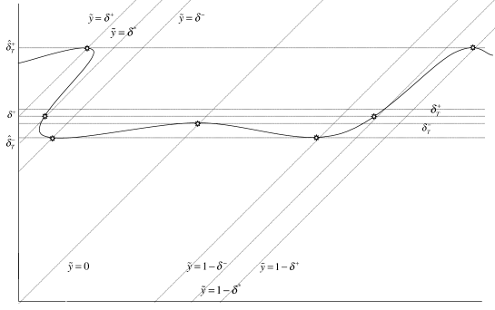
Figure 5. Part of the curve of tangencies

In particular we shall show that $\mathcal{C}^{(1)}$ contains the following points of tangencies $P_{i}(\tilde{y},y)$:

	$P_{1}$	$P_{2}$	$P_{3}$	$P_{4}$	$P_{5}$	$P_{6}$	$P_{7}$	$P_{8}$
$\tilde{y}$	$0$	$\delta^{-}$	$\delta^{*}$	$\delta^{+}$	$1/2$	$1-\delta^{+}$	$1-\delta^{*}$	$1-\delta^{-}$
$y$	$\delta^{-}_{T}$	$\hat{\delta}^{-}_{T}$	$\delta^{+}$	$\hat{\delta}^{+}_{T}$	$\delta^{+}_{T}$	$\hat{\delta}^{+}_{T}$	$\delta^{+}$	$\hat{\delta}^{-}_{T}$

The relative positions of these points is illustrated in Figure 5, notice that the points are indexed according to their ordering along the curve. The relative positions of the horizontal coordinates of the points as as illustrated, in particular $P_{2}$ is the point with the smallest horizontal coordinate, followed by $P_{3}$ followed by $P_{1}$.

2.3. Uniform hyperbolicity away from the critical curves

We recall the basic definitions of a hyperbolic structure. A cone $C\subset\mathbb{R}^{2}$ is a closed convex union of one-dimensional linear subspaces of $\mathbb{R}^{2}$. For a subset $\Lambda\subseteq\mathbb{T}^{2}$, a conefield over $\Lambda$ is a family

$$\mathfrak{C}=\{C(z)\subset T_{z}\mathbb{T}^{2}\}_{z\in\Lambda}$$

of cones lying in the tangent spaces of points in $\Lambda$. We say that the conefield is continuous if the boundaries of the cones vary continuously with the point $z$. We say that the conefield $\mathfrak{C}$ is (strictly) forward invariant under the map $f$ if

$$Df_{z}(C(z))\subset C(f(z))$$

for any $z\in\Lambda$ for which $f(z)\in\Lambda$. Notice that we do not necessarily assume that $\Lambda$ is forward invariant. We say that the conefield $\mathfrak{C}$ is backward invariant if the complementary conefield is “forward” invariant by $Df^{-1}$, i.e. if

$$Df^{-1}_{z}(T_{z}\mathbb{T}^{2}\setminus C(z))\subset T_{f^{-1}(z)}\mathbb{T}^{2}\setminus C(f^{-1}(z))$$

for all $z\in\Lambda$ for which $f^{-1}(z)\in\Lambda$. We say that the (not necessarily invariant) subset $\Lambda\subset\mathbb{T}^{2}$ has a hyperbolic structure if there exists and conefield $\mathfrak{C}$ over $\Lambda$ which is forward and backward invariant and which satisfies the following uniform hyperbolicity properties: there exist constants $C,\lambda>0$ such that

$$\|Df^{\pm n}_{z}(v^{\pm})\|\geq Ce^{\lambda n}\|v^{\pm}\|$$

for vectors $v^{+}\in C(z)$, $v^{-}\in T_{z}\mathbb{T}^{2}\setminus C(z)$ and $n\geq 1$ such that $z,f(z),\ldots,f^{\pm(n-1)}(z)\in\Lambda$.

We now define the regions outside which we have uniform hyperbolicity. For $1\leq m<k$ let

$$\delta^{(\pm m)}=\frac{1}{2\pi}\cos^{-1}\frac{m}{\pi k}$$

and

$$\Delta^{(m)}=\{(x,y):y\notin[\delta^{(-m)},\delta^{(m)}]\cup[1-\delta^{(-m)},1-\delta^{(m)}].$$

We note that for $m$ relatively small, $\Delta^{(m)}$ is not much larger than the strips defined above containing the critical curve. For $m$ relatively large, say $m\approx k^{1-\epsilon}$ the region $\Delta^{(m)}$ is relatively much larger than those strips but still very small.

For an arbitrary point $z\in\mathbb{T}^{2}$ and unit vector $v=(\cos\theta,\sin\theta)$ we write . The following result says that there is a uniformly hyperbolic structure outside $\Delta^{(m)}$ with minimum expansion rate $m$. We suppose here that some large parameter value $k$ has been fixed.

Theorem 3.

Suppose that $k>m\geq 2$, $z\in\mathbb{T}^{2}\setminus\Delta^{(m)}$ and $v=(\cos\theta,\sin\theta)$ with $\tan\theta\in(m^{-1},m)$. Then, letting $Df_{z}(v)=\tilde{v}=(\cos\tilde{\theta},\sin\tilde{\theta})$ we have

$$\tan\tilde{\theta}\in(1-m^{-1},1+m^{-1})\quad\text{ and }\quad\|\tilde{v}\|\geq m.$$

This immediately gives a hyperbolic structure outside $\Delta^{(m)}$ with increasingly strong hyperbolicity as $m$ is chosen large.

3. Forward time foliations

3.1. Definitions and notation

We shall suppose throughout the paper that $k$ is fixed and therefore generally omit it as a subscript in the notation. We shall repeatedly be calculating inverses of trigonometric functions and we therefore fix once and for all the ranges of the inverse functions as follows:

$$\sin^{-1}:[-1,1]\to[-\pi/2,\pi/2],\quad\cos^{-1}:[-1,1]\to[0,\pi],\quad\tan^{-1}:\mathbb{R}\to[-\pi/2,\pi/2].$$

We shall often write unit vectors in the form

$$v=(\cos\theta,\sin\theta)$$

where we always consider $\theta$ to be in the range $[-\pi,\pi]$. We define two polynomial functions

(1) $$\mathcal{P}_{1}(x)=2x^{2}+2x-1\quad\text{ and }\quad\mathcal{P}_{2}(x)=x^{2}+x+1.$$

Notice that their derivatives are

$$\mathcal{P}_{1}^{\prime}(x)=4x+2\quad\text{ and }\quad\mathcal{P}_{2}^{\prime}(x)=2x+1.$$

In particular, $\mathcal{P}_{1}^{\prime}=2\mathcal{P}_{2}^{\prime}$. Moreover, $\mathcal{P}_{1}$ has two real solutions given by

$$x=\frac{-1\pm\sqrt{3}}{2}$$

whereas $\mathcal{P}_{2}$ has no real solutions. We also define

$$\psi_{c}=\psi_{c}(y)=2\pi k\cos(2\pi y)\quad\text{ and }\quad\psi_{s}=\psi_{s}(y)=2\pi k\sin(2\pi y)$$

We then write the derivative of $f$ as

(2) $$Df{(x,y)}=\begin{pmatrix}1&2\pi k\cos(2\pi y)\\ 1&1+2\pi k\cos(2\pi y)\end{pmatrix}=\begin{pmatrix}1&\psi_{c}\\ 1&1+\psi_{c}\end{pmatrix}$$

We also let

$$\varphi=\varphi(y)=-\frac{4\psi_{c}+2}{2\psi_{c}^{2}+2\psi_{c}-1}=-\frac{\mathcal{P}_{1}^{\prime}(\psi_{c})}{\mathcal{P}_{1}(\psi_{c})}.$$

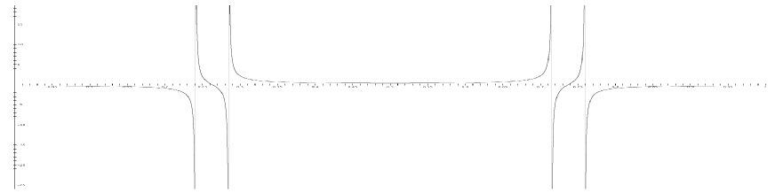
Figure 6. Graph of $\varphi(y)$.

The function $\varphi$ arises naturally and plays an important role in the computation of hyperbolic coordinates and therefore we mention some key properties in the following

Lemma 1.

$\varphi$ has zeros at $\delta^{*}$ and $1-\delta^{*}$, asymptotes at $\delta^{-},\delta^{+},1-\delta^{+},1-\delta^{-}$, where

$$\delta^{\mp}:=\frac{1}{2\pi}\cos^{-1}\frac{-1\pm\sqrt{3}}{4\pi k}\quad\text{ and }\quad\delta^{*}:=\frac{1}{2\pi}\cos^{-1}\frac{-1}{4\pi k}.$$

$\varphi$ also turning points at $0$ and $1/2$, with $\varphi(0)\approx-1/k$ and $\varphi(1/2)\approx 1/k$.

Proof.

Zeroes are given by solutions of $\mathcal{P}_{1}^{\prime}(\psi_{c})=0$. Thus gives $2\psi_{c}+1=0$ and $2\pi k\cos(2\pi y)=-1/2$, and therefore $y=\frac{1}{2\pi}\cos^{-1}\frac{-1}{4\pi k}$. Asymptotes are given by solutions of $\mathcal{P}_{1}(\psi_{c})=2\psi_{c}^{2}+2\psi_{c}-1=0$ and therefore are solutions of $\psi(y)=(-1\pm\sqrt{3})/2$ or $y=\frac{1}{2\pi}\cos^{-1}\frac{-1\pm\sqrt{3}}{4\pi k},$ which are exactly $\delta^{-}$ and $\delta^{+}$. Finally, differentiating $\varphi(y)$ we get

(3) $$\varphi^{\prime}=\frac{d\varphi}{dy}=\frac{d\varphi}{d\psi_{c}}\frac{d\psi_{c}}{dy}=-\frac{\mathcal{P}_{1}^{\prime\prime}\mathcal{P}_{1}-\mathcal{P}_{1}^{\prime 2}}{\mathcal{P}_{1}^{2}}\psi^{\prime}_{c}=\frac{8\mathcal{P}_{2}(\psi_{c})}{\mathcal{P}_{1}(\psi_{c})^{2}}\psi_{c}^{\prime}$$

where the last equality comes from the fact that $\mathcal{P}_{1}^{\prime\prime}\mathcal{P}_{1}-\mathcal{P}_{1}^{\prime 2}=-4(2\psi_{c}^{2}+2\psi_{c}-1)+(4\psi_{c}+2)(4\psi_{c}+2)=8(\psi_{c}^{2}+\psi_{c}+1)$. Since $\mathcal{P}_{2}$ has no real solutions, turning points of $\varphi$ are just the solutions to $\psi_{c}^{\prime}(y)=0$ which is equivalent to $\sin 2\pi y=0$ whose solutions are $y=0$ and $y=1/2$. We have $\psi_{c}(0)=2\pi k$ and $\psi_{c}(1/2)=-2\pi k$ and so

(4) $$\varphi(0)=-\frac{8\pi k+2}{8\pi^{2}k^{2}+2\pi k-1}\approx-\frac{1}{k}\quad\text{ and }\varphi(1/2)=-\frac{-8\pi k+2}{8\pi^{2}k^{2}-2\pi k-1}\approx\frac{1}{k}.$$

∎

We also let

$$\Delta:=[\delta^{-},\delta^{+}].\quad\text{ and }\quad 1-\Delta:=[1-\delta^{+},1-\delta^{-}].$$

We note that $0<\delta^{-}<1/4<\delta^{*}<\delta^{+}<1/2$ and $\delta^{-},\delta^{*},\delta^{+}\to 1/4\text{ as }k\to\infty$. In particular $\Delta$ and $1-\Delta$ shrink as $1/k$ increases and converge to the lines $\{y=1/4\}$ and $\{y=3/4\}$ respectively.

3.2. First order hyperbolic coordinates in forward time

We are now ready to compute precisely the direction of hyperbolic coordinates in forward time. First of all we define

(5) $$\theta^{(1)}(y)=\begin{cases}\pi+\frac{1}{2}\tan^{-1}\varphi(y)&\text{ if }y\in[0,\delta^{-}]\cup[1-\delta^{-},1]\\ \frac{\pi}{2}+\frac{1}{2}\tan^{-1}\varphi(y)&\text{ if }y\in[\delta^{-},\delta^{+}]\cup[1-\delta^{+},1-\delta^{-}]\\ \frac{1}{2}\tan^{-1}\varphi(y)&\text{ if }y\in\left[\delta^{+},1-\delta^{+}\right].\end{cases}$$

Then we have the following

Proposition 1.

For every $k>0$, hyperbolic coordinates for $f_{k}$ are defined at every point of $(x,y)\in\mathbb{T}^{2}$ and depend only on $y$. The vector

$$e^{(1)}(y)=(\cos\theta^{(1)}(y),\sin\theta^{(1)}(y))$$

is a unit vector in the most contracted direction for $Df_{k}$ at $(x,y)$. The most expanded direction is everywhere orthogonal to $e^{(1)}$.

A graph of $\theta^{(1)}(y)$ is shown below. Once again this is shown for clarity for small $k$, as $k$ increases the graph approaches a step function.

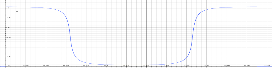
Figure 7. Graph of $\theta^{(1)}(y)$

An analysis of the properties of the function $\theta^{(1)}$ gives the following

Corollary 1.

$e^{(1)}$ rotates monotonically clockwise in $[0,1/2]$ between an angle of $\theta^{(1)}(0)\approx\pi-1/k$ close to the negative horizontal semi-axis at $y=0$ to an angle of $\theta^{(1)}(1/2)\approx 1/k$ close to the positive horizontal semi-axis at $y=1/2$, swinging rapidly between the negative diagonal at $y=\delta^{-}$, through the vertical at $y=\delta^{*}$, to the positive diagonal at $y=\delta^{+}$. Then $e^{(1)}$ rotates monotonically counter-clockwise in $[1/2,1]$ between an angle of $\theta^{(1)}(1/2)\approx 1/k$ close to the positive horizontal semi-axis at $y=1/2$, to and angle $\theta^{(1)}(1)=\theta^{(1)}(0)\approx\pi-1/k$ close to the negative horizontal semi-axis at $y=1=0$, swinging rapidly between the positive diagonal at $y=1-\delta^{+}$, through the vertical at $y=1-\delta^{*}$, to the negative diagonal at $y=1-\delta^{-}$.

Proof of Proposition 1.

We start by showing that hyperbolic coordinates exist for all $k$ and for all points in $\mathbb{T}^{2}$. We then give a general formula for hyperbolic coordinates (which implies in particular that the most contracted and the most expanded directions are always orthogonal). We then substitute the explicit expressions related to our setting into this formula. Finally we establish which of the directions given by the formula is actually the contracting direction and which is the expanding direction.

3.2.1. Existence of hyperbolic coordinates

Since $\det(Df(z))\equiv 1$ it is sufficient to show that for every $k$ and for every point $z\in\mathbb{T}^{2}$ there is some vector $v\in T_{z}\mathbb{T}^{2}$ which is expanding. Indeed, for any $k$ and any $z$ we have

$$\|Df_{z}(1,0)\|=\left\|\begin{pmatrix}1&\psi_{c}\\ 1&1+\psi_{c}\end{pmatrix}\begin{pmatrix}1\\ 0\end{pmatrix}\right\|=\|(1,1)\|=\sqrt{2}>1.$$

3.2.2. General formula for hyperbolic coordinates

Given $z\in\mathbb{T}^{2}$, contracting and expanding directions are computed exactly as follows. Letting $v=(\cos\theta,\sin\theta)$ denote a general vector, the most contracted and most expanded directions are solutions to the differential equation

$$\frac{d\|Df_{z}(\sin\theta,\cos\theta)\|}{d\theta}=0.$$

If the left hand side of this equation is not identically equal to zero, we obtain the relation

(6) $$\tan 2\theta=\frac{2(\partial_{x}f_{1}\partial_{y}f_{1}+\partial_{x}f_{2}\partial_{y}f_{2})}{(\partial_{x}f_{1})^{2}+(\partial_{x}f_{2})^{2}-(\partial_{y}f_{1})^{2}-(\partial_{y}f_{2})^{2}}.$$

Notice that $\tan 2\theta$ is a periodic function with period $\pi/2$ and therefore defines 2 orthogonal directions; it does not, however, distinguish the most contracting from the most expanding direction.

3.2.3. Specific formula for hyperbolic coordinates

We can now substitute the partial derivatives of $f$ into (6). Since the derivative of $f$ depends only on the $y$ coordinate, it follows that the hyperbolic coordinates depend only on $y$. Using the definition of $\varphi$, we get

(7) $$\tan{2\theta(z)}=\frac{2(\psi_{c}+1+\psi_{c})}{1+1-\psi_{c}^{2}-(1+\psi_{c})^{2}}=\frac{2(2\psi_{c}+1)}{1-2\psi_{c}(\psi_{c}+1)}=\varphi(y)$$

As mentioned above, this equation defines two orthogonal directions without distinguishing the expanding and the contracting one. Naively inverting $\tan$ to get

(8) $$\theta=\frac{1}{2}\tan^{-1}\varphi(y)$$

fixes one of these solutions, namely the one belonging to $(-\pi/4,\pi/4)$, which, in general, may be a contracting or an expanding direction. Moreover, as $y$ changes, the hyperbolic coordinates change and equation (8) may pick out the contracting directions for some values of $y$ and the expanding directions for others.

3.2.4. Establishing the contracting and the expanding directions

We fix first of all a single value of $y$, for simplicity let $y=0$. From (4) we have $\varphi(0)\approx-1/k$ for large $k$, and therefore, from (8),

$$\theta(0)=\frac{1}{2}\tan^{-1}\left(-\frac{1}{k}\right)\approx-\frac{1}{k}.$$

This means that one of the solutions of (7) has very small negative slope. A simple calculation shows that this is indeed the contracting direction. To see this we shall show that every vector $v=(\cos\theta,\sin\theta)$ with $\theta\in(\pi/4,3\pi/4)$ is significantly expanded: recall first that for $y=0$ we have $\psi_{c}(0)=2\pi k\cos 0=2\pi k$, then for all $\iota\in(-1,1)$ we have

$$\|Df_{y=0}(\iota,1)\|=\left\|\begin{pmatrix}1&\psi_{c}\\ 1&1+\psi_{c}\end{pmatrix}\begin{pmatrix}\iota\\ 1\end{pmatrix}\right\|=\left\|\begin{pmatrix}\iota+2\pi k\\ \iota+1+2\pi k\end{pmatrix}\right\|\gtrsim k$$

This implies that the contracting direction is actually almost horizontal (and with negative slope). We now have two choices for defining $\theta^{(1)}$ and the unit vector $e^{(1)}$. It seems simpler, for the rest of the discussion to choose $\theta^{(1)}=\pi+\frac{1}{2}\tan^{-1}\varphi(0)$ giving a most contracted unit vector close to the negative horizontal semi-axis.

3.2.5. Analytic continuation of the most contracted direction

To obtain a complete formula for $\theta^{(1)}$ we need to keep track of the rotation of $e^{(1)}$ as $y$ increases. Indeed, if the hyperbolic coordinates changed direction so that the most expanded direction corresponded to angles $\theta\in(-\pi/4,\pi/4)$ then the formula would start picking up the wrong direction.

We observe therefore first of all that $\varphi$ is decreasing in $y$ at $y=0$ and that this corresponds to a clockwise rotation of $e^{(1)}$ as $y$ increases near 0. For $y=\delta^{-}$ we have $|\varphi(y)|=\infty$ which corresponds to the hyperbolic coordinates being aligned with the diagonal. As $y$ crosses $\delta^{-1}$, the equation $\frac{1}{2}\tan^{-1}\varphi(y)$ which always only picks up the solution inside $[-\pi/4,\pi/4]$ switches from picking up one of the most contracting directions to picking up one of the most expanding directions. To realize the continuity of $e^{(1)}$ (hyperbolic coordinates depend smoothly on the position) we change the definition to $\theta^{(1)}=\frac{\pi}{2}+\frac{1}{2}\tan^{-1}(\varphi(y))$. A similar change occurs as $y$ crosses $\delta^{+}$ and then $1-\delta^{+}$ and $1-\delta^{-}$. ∎

3.2.6. Geometry of the most contacting direction

A more detailed analysis along the lines of the arguments given above, allow us to give a detailed description of how that most contracting unit vector $e^{(1)}$ depends on the point $y$.

Proof of Corollary 1.

To find the turning points of $\theta^{(1)}$ we calculate derivatives with respect to $y$ and get

$$\frac{d\theta^{(1)}}{dy}=\frac{1}{2}\frac{\varphi^{\prime}}{(1+\varphi^{2})}.$$

From the proof of Proposition 1 we have that the only zeros of $\varphi^{\prime}$ are $y=0$ and $y=1/2$. Moreover, at $y=0$ we have $\psi_{c}(y)=2\pi k\cos(2\pi y)=2\pi k$ and therefore

$$\theta^{(1)}(0)=\pi+\frac{1}{2}\tan^{-1}\frac{8\pi k+2}{1-8\pi^{2}k^{2}-4\pi k}\approx\pi-\frac{1}{k}$$

and st $y=1/2$ we have $\psi_{c}(y)=-2\pi k$ and therefore

$$\theta^{(1)}\left(\frac{1}{2}\right)=\frac{1}{2}\tan^{-1}\frac{-8\pi k+2}{1-8\pi^{2}k^{2}+4\pi k}\approx\frac{1}{k}$$

For $y$ equal to $\delta^{\pm},1-\delta^{\pm}$ we have $|\varphi(y)|=\infty$ which corresponds precisely to being aligned with the diagonals as stated. For $y$ equals $\delta^{*}$ and $1-\delta^{*}$ we have $\varphi(y)=0$ which corresponds precisely to $e^{(1)}(y)$ being vertical as stated.

∎

3.3. First order foliations in forward time

The geometry of the stable and unstable foliations $\mathcal{E}^{(1)}$ and $\mathcal{F}^{(1)}$ now follows by a careful consideration of the position of the vectors $e^{(1)}$ as described in Corollary 1.

4. Backward time foliations

We now carry out an analogous analysis of the inverse map

(9) $$f_{k}^{-1}\begin{pmatrix}x\\ y\end{pmatrix}=\begin{pmatrix}x-k\sin 2\pi(y-x)\\ y-x\end{pmatrix}\mod 1$$

in order to obtain the contracting and expanding foliations $\mathcal{E}^{(-1)}$ and $\mathcal{F}^{(-1)}$ in backward time.

4.1. Definitions and notation

Hyperbolic coordinates in backward time are constant along “diagonals”, i.e. lines of slope 1. We therefore start by introducing a notations which will simplify our analysis: let

$$\tilde{y}=y-x\mod 1.$$

Lines of the form $\{\tilde{y}=c\}$ have unit slope and intersect the $y$-axis at $y=c$. Thus, when it is convenient to do so, we will write the coordinates of a point in the form $(\tilde{y},y)$ meaning that this point lies at the intersection of the horizontal line through $(0,y)$ (in standard coordinates) with the diagonal through $(0,\tilde{y})$ (in standard coordinates). We shall often switch between standard and diagonal coordinates sometimes even using both within the same expression. To avoid confusion we shall use a  $\tilde{}$   to indicate variables and functions of variables in “diagonal coordinates”. We let

$$\tilde{\psi}_{c}=2\pi k\cos(2\pi\tilde{y})\quad\text{ and }\quad\tilde{\psi}_{s}=2\pi k\sin(2\pi\tilde{y})$$

and write the derivative of $f^{-1}$ as

$$Df_{k}^{-1}(x,y)=\begin{pmatrix}1+2\pi k\cos(2\pi(y-x))&-2\pi k\cos(2\pi(y-x))\\ -1&1\end{pmatrix}=\begin{pmatrix}1+\tilde{\psi}_{c}&-\tilde{\psi}_{c}\\ -1&1\end{pmatrix}.$$

We also define

$$\tilde{\varphi}=\tilde{\varphi}(\tilde{y})=-\frac{2(\tilde{\psi}_{c}^{2}+\tilde{\psi}_{c}+1)}{1+2\tilde{\psi}_{c}}=-\frac{2\mathcal{P}_{2}(\tilde{\psi}_{c})}{\mathcal{P}_{2}^{\prime}(\tilde{\psi}_{c})}$$

The graph of $\tilde{\varphi}(\tilde{y}))$ is sketched in Figure 8 below.

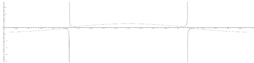
Figure 8. Graph of $\tilde{\varphi}(\tilde{y})$.

Lemma 2.

$\tilde{\varphi}$ has no zeroes, two asymptotes, at $\delta^{*}$ and $1-\delta^{*}$, and six turning points, at $0,\delta^{-},\delta^{+},1/2,1-\delta^{+},1-\delta^{-}$, with

$$\tilde{\varphi}(0)\approx-k,\quad\tilde{\varphi}(1/2)\approx k,$$

and

$$\tilde{\varphi}(\delta^{-})=\tilde{\varphi}(1-\delta^{-})=-\frac{\sqrt{3}}{2},\quad\tilde{\varphi}(\delta^{+})=\tilde{\varphi}(1-\delta^{+})=\frac{\sqrt{3}}{2}.$$

We note that the value of $\tilde{\varphi}$ at the turning points $\delta^{\pm}$ and $1-\delta^{\pm}$ do not depend on $k$, whereas the values at the turning points $0,1/2$ do depend on $k$ and approach $\pm\infty$ as $k\to\infty$.

Proof.

$\tilde{\varphi}$ has no zeros since $\mathcal{P}_{2}$ has no real solutions. Asymptotes are solutions of $\mathcal{P}_{2}^{\prime}(\psi_{c})=0$ which amounts to $\tilde{\psi}(\tilde{y})=-{1}/{2}$ or $\tilde{y}=\frac{1}{2}\cos^{-1}{-\frac{1}{4\pi k}}$, which correspond precisely to $\tilde{y}=\delta^{*}$ and $\tilde{y}=1-\delta^{*}$. To compute the turning points of $\tilde{\varphi}$ we differentiate to get

(10) $$\tilde{\varphi}^{\prime}=\frac{d\tilde{\varphi}}{d\tilde{y}}=\frac{d\tilde{\varphi}}{d\tilde{\psi}_{c}}\frac{d\tilde{\psi}_{c}}{d\tilde{y}}=\frac{2(\mathcal{P}_{2}^{\prime 2}-\mathcal{P}_{2}\mathcal{P}_{2}^{\prime})}{\mathcal{P}_{2}^{\prime 2}}\frac{d\tilde{\psi}_{c}}{d\tilde{y}}=\frac{2\mathcal{P}_{1}(\tilde{\psi}_{c})}{\mathcal{P}_{2}^{\prime 2}(\tilde{\psi}_{c})}\tilde{\psi}_{c}^{\prime}$$

where $\mathcal{P}_{2}^{\prime 2}-\mathcal{P}_{2}\mathcal{P}_{2}^{\prime\prime}=(2\tilde{\psi}_{c}+1)^{2}-2(\tilde{\psi}_{c}^{2}+\tilde{\psi}_{c}+1)=2\tilde{\psi}_{c}^{2}+2\tilde{\psi}_{c}-1=\mathcal{P}_{1}(\tilde{\psi}_{c})$ and $\tilde{\psi}^{\prime}(\tilde{y})=(2\pi)^{2}k\sin(2\pi\tilde{y}).$ Therefore $\tilde{\varphi}^{\prime}=0$ if $2\psi^{2}+2\psi-1=0$ which gives $\psi(\tilde{y})=-(1\pm\sqrt{3})/2$ and thus $\tilde{y}=\{\delta^{-},\delta^{+},1-\delta^{+},1-\delta^{-}\}$ or $\tilde{\psi}^{\prime}=0$ which gives $\tilde{y}=\sin^{-1}0=\{0,1/2\}.$ To compute the images of these turning points, we have $\tilde{\psi}(0)=2\pi k$ and $\tilde{\psi}(1/2)=12\pi k$ and so $\tilde{\varphi}(0)\approx-k$ and $\tilde{\varphi}(1/2)\approx-k.$ By the definition of $\tilde{\psi}$ we can compute $\tilde{\psi}(\delta^{-})=2\pi k\cos\left(2\pi\left(\tfrac{1}{2\pi}\cos^{-1}((-1+\sqrt{3})/(4\pi k))\right)\right)=(-1+\sqrt{3})/2$ and also $\tilde{\psi}(\delta^{+})=2\pi k\cos\left(2\pi\left(\frac{1}{2\pi}\cos^{-1}(-1-\sqrt{3})/(4\pi k)\right)\right)=-(1+\sqrt{3})/(2)$. Therefore so $\tilde{\varphi}(\delta^{-})=-(\tilde{\psi}^{2}+\tilde{\psi}+1)/(1+2\tilde{\psi})=-\sqrt{3}/2$ and $\tilde{\varphi}(\delta^{+})=\sqrt{3}/2$ as required. ∎

4.2. First order hyperbolic coordinates in backward time

We are now ready to compute hyperbolic coordinates in backward time. First of all we define

(11) $$\theta^{(-1)}(\tilde{y})=\begin{cases}\frac{\pi}{2}+\frac{1}{2}\tan^{-1}(\tilde{\varphi}(\tilde{y}))&\text{ if }\tilde{y}\in[0,\delta^{*}]\cup[1-\delta^{*},1]\\ \frac{1}{2}\tan^{-1}(\tilde{\varphi}(\tilde{y}))&\text{ if }\tilde{y}\in[\delta^{*},1-\delta^{*}]\end{cases}$$

Then we have the following

Proposition 2.

For every $k>0$, hyperbolic coordinates for $f_{k}^{-1}$ are defined at every point $(x,y)\in\mathbb{T}^{2}$ and depend only on $\tilde{y}$. The vector

$$e^{(-1)}(z)=(\sin\theta^{(-1)}(\tilde{y}),\cos\theta^{-1}(\tilde{y}))$$

is a unit vector in the most contracted direction for $Df_{k}^{-1}$ at $(x,y)$.

A graph of $\theta^{(-1)}(\tilde{y})$ is shown in Figure 9 below.

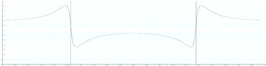
Figure 9. Graph of $\theta^{(-1)}(\tilde{y})$.

Corollary 2.

$e^{(-1)}$ rotates counter-clockwise in $(0,\delta^{-1})$ from $\theta^{(-1)}(0)\gtrsim\pi/4$ (just above the positive diagonal) for $\tilde{y}=0$, with $\theta^{(-1)}(0)\searrow\pi/4$ as $k\to\infty$, to an angle $\theta^{(-1)}(\delta^{-})\gtrsim 3\pi/8$, independent of $k$, then swings rapidly clockwise in $(\delta^{-},\delta^{+})$ to an angle $\theta^{(-1)}(\delta^{+})\lesssim\pi/8$, independent of $k$, crossing the positive diagonal at $\tilde{y}=\delta^{*}$, then rotates counter-clockwise in $(\delta^{+},1/2)$ to an angle $\theta^{(-1)}(1/2)\lesssim\pi/4$ (just below the positive diagonal) with $\theta^{(-1)}(1/2)\nearrow\pi/4$ as $k\to\infty$. The process continues in $(1/2,1)$ in reverse in a perfectly symmetric manner.

Proof of Proposition 2.

The argument follows along the same lines as the proof of Proposition 1. The existence of hyperbolic coordinates everywhere follows directly from the analogous statement in forward time since $e^{(-1)}(z)$ is exactly the image of the most expanded direction $f^{(1)}(f^{-1}(z))$ under $Df_{f^{-1}(z)}$. Then, substituting the corresponding partial derivatives into (6) we get

$$\tan 2\theta=\frac{2(-\tilde{\psi}_{c}(1+\tilde{\psi}_{c})-1)}{(1+\tilde{\psi}_{c})^{2}+1-\tilde{\psi}_{c}^{2}-1}=-\frac{2(\tilde{\psi}_{c}^{2}+\tilde{\psi}_{c}+1)}{2\tilde{\psi}_{c}+1}=\tilde{\varphi}(\tilde{y}).$$

For $\tilde{y}=0$ we have $\tilde{\psi}_{c}=2\pi k\cos 2\pi 0=2\pi k$ and so this gives $\tan 2\theta=-2(4\pi^{2}k^{2}+2\pi k+1)/(4\pi k+1)\to-\infty$ as $k\to\infty$ and so, taking $\tan^{-1}$ on both sides, this gives $\theta\gtrsim-\pi/4$ with $\theta\searrow-\pi/4$ as $k\to\infty$. Thus, for large $k$, the hyperbolic coordinates are almost aligned with the diagonals. To establish which direction is contacted and which direction expanded we note first of all that for $\tilde{\psi}_{c}(0)=2\pi k$ and therefore, applying the derivative at $\tilde{y}=0$ to a vector which is close to the negative diagonal we get

$$Df_{\tilde{y}=0}^{-1}(1\pm\varepsilon,-1)=\begin{pmatrix}1+\tilde{\psi}_{c}&-\tilde{\psi}_{c}\\ -1&1\end{pmatrix}\begin{pmatrix}1\pm\varepsilon\\ -1\end{pmatrix}=\begin{pmatrix}1+2\pi k&-2\pi k\\ -1&1\end{pmatrix}\begin{pmatrix}1\pm\varepsilon\\ -1\end{pmatrix}\approx\begin{pmatrix}4\pi k\\ -2\end{pmatrix}$$

The region around the negative diagonal is therefore clearly not the contracting direction, and thus we define $\theta^{(-1)}(0)=\pi/2+\tan^{-1}\tilde{\varphi}(0)$. Since the most contracting direction depends smoothly on $\tilde{y}$ this definition continues to work as long as the hyperbolic coordinates do not swing “through” the diagonals, which happens exactly when $\tan 2\theta=\pm\infty$ or $2\tilde{\psi}_{c}+1=0$, i.e. for $\tilde{y}=\delta^{*}$ and $\tilde{y}=1-\delta^{*}$. Between these two points the formula picks up the contracting direction, which now lies in the correct quadrant, and we obtain the statement with the definition of $\theta^{(-1)}$ as given above. ∎

4.2.1. Geometry of the most contracting directions in backward time

As in the forward time case, we now carry out a more detailed analysis of the function $e^{(-1)}$ to determine the variation of $\theta^{(-1)}$ on $\tilde{y}$.

Proof of Corollary 2.

To find the turning points of $\theta^{(-1)}$ we calculate the derivative. From (10) we have

$$\frac{d\theta^{(-1)}}{dy}=\frac{1}{2}\frac{\tilde{\varphi}^{\prime}}{1+\tilde{\varphi}^{2}}=\frac{\mathcal{P}_{1}(\tilde{\psi}_{c})\tilde{\psi}_{c}^{\prime}}{\mathcal{P}_{2}^{\prime 2}(1+\tilde{\varphi}^{2})}$$

which immediately gives the six turning points at $0,1/2$ from $\tilde{\psi}_{c}=0$ and at $\delta^{-},\delta^{+},1-\delta^{-}$ and $1-\delta^{+}$ from $\mathcal{P}_{1}=0$. We compute the value of $\theta^{(-1)}$ at these turning points. At $\tilde{y}=0$ we have $\tilde{\psi}(0)=2\pi k$ and $\tilde{\varphi}(0)\approx-k$ and therefore, from (11),

$$\theta^{(-1)}(0)=\frac{\pi}{2}+\frac{1}{2}\tan^{-1}(\tilde{\varphi}(0))\gtrsim\frac{\pi}{2}+\frac{1}{2}\tan^{-1}(-k)\gtrsim\frac{\pi}{4}.$$

Thus $e^{(-1)}$ lies just slightly above the positive diagonal, tending to the positive diagonal as $k$ increases. For $\tilde{y}$ between $0$ and $\tilde{y}=\delta^{-}$, $\tilde{\varphi}(\tilde{y})$ increases and $e^{(-1)}$ rotates counterclockwise. At $\tilde{y}=\delta^{-}$ (and $\tilde{y}=1-\delta^{-}$) we have (see Lemma 2) $\tilde{\varphi}(\delta^{-})=-\sqrt{3}/2$ and so

$$\theta^{(-1)}=\frac{\pi}{2}+\frac{1}{2}\tan^{-1}\left(-\frac{\sqrt{3}}{2}\right)\gtrapprox\frac{\pi}{2}-\frac{\pi}{8}=\frac{3\pi}{8}$$

We emphasize that this value is independent of $k$. Past $\delta^{-}$, $\tilde{\varphi}(\tilde{y})$ decreases and $e^{(-1)}$ rotates clockwise. At $\tilde{y}=\delta^{+}$ (and $\tilde{y}=1-\delta^{+}$) we have $\tilde{\varphi}(\delta^{+})=\sqrt{3}/2$ and so

$$\theta^{(-1)}=\frac{1}{2}\tan^{-1}\frac{\sqrt{3}}{2}\lessapprox\frac{\pi}{8}.$$

This value is also independent of $k$ so the vector $e^{(-1)}$ swings through a fixed angle of almost $\pi/4$ as $\tilde{y}$ ranges in the interval $[\delta^{-},\delta^{+}]$ whose length of the order $1/k$ and which shrinks to 0 as $k\to\infty$. Finally, the direction of $e^{(-1)}$ changes again and now rotates in a counter-clockwise sense. At $\tilde{y}=1/2$ we have $\tilde{\varphi}\approx-k$ and so

$$\theta^{(-1)}(1/2)=\frac{1}{2}\tan^{-1}(\tilde{\varphi}(1/2))\lessapprox\frac{1}{2}\tan^{-1}k\lessapprox\frac{\pi}{4}.$$

∎

4.3. First order foliations in backwards time

The geometry of the stable and unstable foliations $\mathcal{E}^{(-1)}$ and $\mathcal{F}^{(-1)}$ now follows by a careful consideration of the position of the vectors $e^{(-1)}$ as described in Corollary 2.

5. Curves of tangencies

In this section we prove Theorem 2. Recall first of all that $\mathcal{C}^{(1)}$ is, by definition, the locus of points $z$ for which

(12) $$e^{(1)}(z)=e^{(-1)}(z).$$

Our strategy is to obtain an explicit formula for this set by equating the explicit formulas for $e^{(1)}(z)$ and $e^{(-1)}(z)$, although we emphasize that this does not follow simply by substituting the corresponding expressions into (12) as they are piecewise defined in various regions of the torus and also $e^{(1)}$ is given as a function of $y$ whereas $e^{(-1)}$ is given as a function of $\tilde{y}$; some non-trivial analysis is therefore required. We shall continue to use the definitions and notation of the previous section, although we recall some of the definitions here for clarity. First of all, writing $e^{(1)}=(\cos\theta^{(1)},\sin\theta^{(1)})$ and $e^{(-1)}=(\cos\theta^{(-1)},\sin\theta^{(-1)})$ the equation $e^{(1)}(z)=e^{(-1)}(z)$ reduces to the equation

(13) $$\theta^{(1)}(z)=\theta^{(-1)}(z).$$

We start by dividing the torus $\mathbb{T}^{2}$ into two regions. In one region we show directly that no tangencies can occur, in the other we show that they can be computed through a simplified formula.

Lemma 3.

There are no tangencies in $\{(x,y)\in\mathbb{T}^{2}:y\in[0,\delta^{-}]\cup[1-\delta^{-},1]\}$.

Proof.

From the equations defining the contracting directions $e^{(1)}$ and $e^{(-1)}$ it follows that $e^{(-1)}$ always lies in the $\{x>0,y>0\}$ quadrant whereas, for $y\in[0,\delta^{-}]\cup[1-\delta^{-},1]$ the vector $e^{(-1)}$ lies in the quadrant $\{x<0,y>0\}$. Thus they can never be aligned and there can be no tangencies in this region. ∎

Lemma 4.

Tangencies in $\{(x,y):y\in[\delta^{-},1-\delta^{-}]\}$ are given by solutions to $\varphi(y)=\tilde{\varphi}(\tilde{y})$.

Proof.

We divide the region $\{(x,y):y\in[\delta^{-},1-\delta^{-}]\}$ into two parts as follows:

$$\mathcal{R}_{1} =\{(x,y):y\in[\delta^{-},\delta^{+}]\cup[1-\delta^{+},1-\delta^{-}],\tilde{y}\in[0,\delta^{*}]\cup[1-\delta^{*},1]\},$$

$$\mathcal{R}_{2} =\{(x,y):y\in(\delta^{+},1-\delta^{+}],\tilde{y}\in[\delta^{*},1-\delta^{*}]\}$$

It then just remains to notice that these the definitions of $\theta^{(1)}$ and $\theta^{(-1)}$ give $\theta^{(1)}=\theta^{(-1)}$ if and only if $\varphi(y)=\tilde{\varphi}(\tilde{y})$ precisely when $(x,y)\in\mathcal{R}_{1}\cup\mathcal{R}_{2}$. ∎

Proof of Theorem 2.

From the previous discussion it follows that we just need to solve the equation

(14) $$\varphi(y)=\tilde{\varphi}(\tilde{y}).$$

Figure 10 shows the graphs of these two functions side by side.

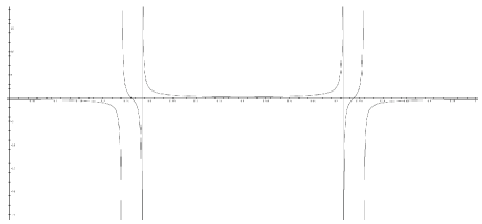
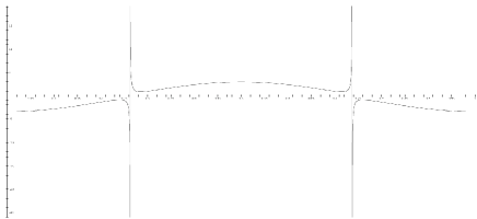
Figure 10. Graph of $\varphi(y)$ and $\tilde{\varphi}(\tilde{y})$.

Notice that we need to consider the two regions $\mathcal{R}_{1}$ and $\mathcal{R}_{2}$ separately. These regions are easily defined in both graphs by the asymptotes which occur at $\delta^{-},\delta^{+},1=\delta^{+},1-\delta^{-}$ for $\varphi$ and $\delta^{*},1-\delta^{*}$ for $\tilde{\varphi}$. Equation (14) can be written as

$$y=\varphi^{-1}(\tilde{\varphi}(\tilde{y})$$

where the appropriate inverse branch is considered depending on the value of $\tilde{y}$ so that we have

(15) $$y=\begin{cases}\varphi^{-1}(\tilde{\varphi}(\tilde{y}))\cap[\delta^{-},\delta^{+}]\cup[1-\delta^{+},1-\delta^{-}]&\text{ if }\tilde{y}\in[0,\delta^{*}]\cup[1-\delta^{*},1]\\ \varphi^{-1}(\tilde{\varphi}(\tilde{y}))\cap[\delta^{+},1-\delta^{+}]&\text{ if }\tilde{y}\in[\delta^{*},1-\delta^{*}].\end{cases}$$

Notice that in both cases we get exactly two solutions corresponding to the two curves of tangencies. To calculate a more explicit expression for this we compute $\varphi^{-1}$ explicitly. Writing

$$\varphi(y)=-\frac{4\psi_{c}+2}{2\psi_{c}^{2}+2\psi_{c}-1}=z$$

This gives the quadratic equation $2z\psi_{c}^{2}+2(z+2)\psi_{c}-z+2=0$ in $\psi_{c}$. Solving for $\psi_{c}$ this gives

$$\psi_{c}=\frac{-2(z+2)\pm\sqrt{4(z+2)^{2}+8z(z-2)}}{4z}=\frac{-(z+2)\pm\sqrt{3z^{2}+4}}{2z}$$

From the definition of $\psi_{c}=\psi_{c}(y)=2\pi k\cos(2\pi y)$ we then get

(16) $$y=\varphi^{-1}(z)=\frac{1}{2\pi}\cos^{-1}\frac{-(z+2)\pm\sqrt{3z^{2}+4}}{4\pi kz}$$

Notice that the expression under the square root is always positive. The last thing to check is that the curves are contained in the two thin strips as stated in the Theorem. To show this we now define the values of $\hat{\delta}_{T}^{-},\delta_{T}^{-},\delta_{T}^{+},\hat{\delta}_{T}^{+}$ as

$$\hat{\delta}_{T}^{-}:=\varphi^{-1}(\tilde{\varphi}(\delta^{-}))\cap[\delta^{-},\delta^{+}]$$

$$\hat{\delta}_{T}^{+}:=\varphi^{-1}(\tilde{\varphi}(\delta^{+}))\cap[\delta^{+},1/2]$$

$$\delta_{T}^{-}:=\varphi^{-1}(\tilde{\varphi}(0))\cap[\delta^{-},\delta^{+}]$$

$$\delta_{T}^{+}:=\varphi^{-1}(\tilde{\varphi}(1/2))\cap[\delta^{+},1/2].$$

Figure 11.

It then follows, just by the geometry of the graphs of $\varphi$ and $\tilde{\varphi}$, see Figure 11, that

$$\delta^{-}<1/4<\delta^{*}<\hat{\delta}_{T}^{-}<\delta_{T}^{-}<\delta^{+}<\delta_{T}^{+}<\hat{\delta}_{T}^{+}$$

and that all these constants tend to $1/4$ (and thus to each other) as $k\to\infty$ (although we shall not use this in any significant way, notice nonetheless that $|\delta^{+}_{T}-\delta^{-}_{T}|\approx 1/k^{2}$ whereas $|\hat{\delta}^{+}_{T}-\hat{\delta}^{-}_{T}|\approx 1/k$). The statement then follows from an analysis of the graph in Figure 10, the formula (15), and the definitions made above. Indeed, notice that as $\tilde{y}$ ranges over the interval $[0,\delta^{*}]$ the lowest value attained by $y=\varphi^{-1}(\tilde{\varphi}(\tilde{y}))$ restricted to $[\delta^{-},\delta^{+}]$ is precisely $\hat{\delta}^{-}_{T}$ which is attained at the point $\tilde{y}=\delta^{-}$ where $\tilde{\varphi}$ has a local maximum. Similarly, as $\tilde{y}$ ranges over the interval $[\delta^{*},1/2]$, the highest value attained by $y=\varphi^{-1}(\tilde{\varphi}(\tilde{y}))$ restricted to $[\delta^{+},1/2]$ is precisely $\hat{\delta}^{+}_{T}$ which is attained at the point $\tilde{y}=\delta^{+}$ which is where $\tilde{\varphi}$ has a local maximum. Exactly the same analysis works for the other regions. This completes the proof of Theorem 2. ∎

Before ending this section, we use the formula we have obtained to compute a few explicit points on the curve of tangency to obtain Figure 5. From the definitions above we immediately have an explicitly defined set of tangencies which includes the following points which we express in $(\tilde{y},y)$ coordinates:

$\tilde{y}$	$0$	$\delta^{-}$	$\delta^{*}$	$\delta^{+}$	$1/2$	$1-\delta^{+}$	$1-\delta^{*}$	$1-\delta^{-}$
$y$	$\delta^{-}_{T}$	$\hat{\delta}^{-}_{T}$	$\delta^{+}$	$\hat{\delta}^{+}_{T}$	$\delta^{+}_{T}$	$\hat{\delta}^{+}_{T}$	$\delta^{+}$	$\hat{\delta}^{-}_{T}$

Notice that for large $k$ the argument of $\cos^{-1}$ is close to $0$. Thus, using the fact that $\cos^{\prime}(0)=-1$ we immediately have the following limits as $k\to\infty$:

$$\delta^{-}(k)\to\frac{1}{4}-\frac{\sqrt{3}-1}{8\pi^{2}k};\delta^{*}(k)\to\frac{1}{4}+\frac{1}{8\pi^{2}k};\delta^{+}(k)\to\frac{1}{4}+\frac{1+\sqrt{3}}{8\pi^{2}k};$$

$$\hat{\delta}^{-}_{T}\to\frac{1}{4}+\frac{1+\sqrt{3}/3}{8\pi^{2}k};\hat{\delta}^{+}_{T}\to\frac{1}{4}+\frac{1+3\sqrt{3}}{8\pi^{2}k}.$$

In particular this allows us to study the positions of various points. We have

$$\delta^{+}-\delta^{*}\to\frac{\sqrt{3}}{8\pi^{2}k};\quad\hat{\delta}^{-}_{T}-\delta^{-}\to\frac{\frac{4}{3}\sqrt{3}}{8\pi^{2}k}\quad\hat{\delta}^{+}_{T}-\delta^{+}\to\frac{2\sqrt{3}}{8\pi^{2}k};$$

This implies the relative positions as illustrated in Figure 5.

6. Uniform hyperbolicity

In this section we prove Theorem 3. We divide the proof into two parts, estimating the direction of $\tilde{v}$ and its magnitude respectively. First of all, however, we mention a couple of elementary consequences of our assumptions on the location of $z$ and the direction of $v$. From the definition of $\psi_{c}$ we have

$$\psi_{c}(\delta^{(\pm m)})=2\pi k\cos\left(2\pi\left(\frac{1}{2\pi}\cos^{-1}\frac{\pm m}{\pi k}\right)\right)=\pm 2m$$

and therefore, $z\notin\Delta^{(m)}$ implies

$$|\psi_{c}|>2m.$$

Also, from our assumptions $\tan\theta\in(m^{-1},m)$ for the direction of $v$ and $m\geq 2$ we get

$$m^{-1}\sin\theta<\cos\theta<m\sin\theta\quad\text{ and }\quad\sin\theta>m^{-1}/2.$$

6.1. Direction

To estimate the direction of the image vector $\tilde{v}=Df_{z}(v)=(\cos\tilde{\theta},\sin\tilde{\theta})$ we recall that the derivative of the standard map $f=f_{k}$ at a point $z=(x,y)$ depends only on $y$ and is

$$Df_{y}=\begin{pmatrix}1&2\pi k\cos(2\pi y)\\ 1&1+2\pi k\cos(2\pi y)\end{pmatrix}=\begin{pmatrix}1&\psi_{c}\\ 1&1+\psi_{c}\end{pmatrix}$$

Thus the image $\tilde{v}=(\cos\tilde{\theta},\sin\tilde{\theta})$ of a generic vector $v=(\cos\theta,\sin\theta)$ is

$$\begin{pmatrix}\cos\tilde{\theta}\\ \sin\tilde{\theta}\end{pmatrix}=Df_{y}\begin{pmatrix}\cos\theta\\ \sin\theta\end{pmatrix}=\begin{pmatrix}1&\psi_{c}\\ 1&1+\psi_{c}\end{pmatrix}\begin{pmatrix}\cos\theta\\ \sin\theta\end{pmatrix}=\begin{pmatrix}\cos\theta+\psi_{c}\sin\theta\\ \cos\theta+(1+\psi_{c})\sin\theta\end{pmatrix}$$

Therefore

(17) $$\tilde{\theta}=\tan^{-1}\left(\frac{\cos\theta+(1+\psi_{c})\sin\theta}{\cos\theta+\psi_{c}\sin\theta}\right)=\tan^{-1}\left(1+\frac{\sin\theta}{\cos\theta+\psi_{c}\sin\theta}\right)$$

Therefore it is sufficient to bound the absolute value of the fraction ${\sin\theta}/{(\cos\theta+\psi_{c}\sin\theta)}$ by $m^{-1}$. From the condition $\tan\theta\in(m^{-1},m)$ we know that $\sin\theta$ and $\cos\theta$ have the same sign. Suppose without loss of generality that $\sin\theta>0$ and $\cos\theta>0$. We consider two different cases, corresponding to different regions of $\mathbb{T}^{2}\setminus\Delta^{(m)}$. If $\psi=\psi_{c}(y)>0$ we have

$$\frac{|\sin\theta|}{|\cos\theta+\psi\sin\theta|}=\frac{\sin\theta}{\cos\theta+\psi\sin\theta}\leq\frac{\sin\theta}{\psi_{c}\sin\theta}=\frac{1}{\psi}\leq\frac{1}{2m}<m^{-1}.$$

If $\psi=\psi_{c}(y)<0$ we distinguish two further subcases. If $\cos\theta-|\psi|\sin\theta\geq 0$ then $\cos\theta-|\psi|\sin\theta>m^{-1}\sin\theta-|\psi|\sin\theta=(m^{-1}-|\psi|)\sin\theta$ and therefore

$$\frac{|\sin\theta|}{|\cos\theta+\psi\sin\theta|}=\frac{\sin\theta}{\cos\theta-|\psi|\sin\theta}\leq\frac{\sin\theta}{(m^{-1}-|\psi|)\sin\theta}=\frac{1}{m^{-1}-|\psi|}<\frac{1}{m}.$$

If $\cos\theta-|\psi|\sin\theta\leq 0$ then $\cos\theta-|\psi|\sin\theta\leq m\sin\theta-|\psi|\sin\theta=(m-|\psi|)\sin\theta$ and so $|\cos\theta-|\psi\sin\theta|\geq(m-|\psi|)\sin\theta$ and therefore

$$\frac{|\sin\theta|}{|\cos\theta+\psi\sin\theta|}=\frac{\sin\theta}{|\cos\theta-|\psi|\sin\theta|}\leq\frac{\sin\theta}{|m-|\psi||\sin\theta}=\frac{1}{|m-|\psi||}\leq\frac{1}{m}.$$

This completes the proof of the invariance of the conefield.

Remark 1.

Note that the formula (17) describes a general relation between the angle $\theta$ of a vector $v$, the point $z$, and the angle $\tilde{\theta}$ of the image vector $\tilde{v}=Df_{z}(v)$ (in particular it holds for every $\theta$ and every $z$). We mention here two simply but possibly interesting consequences of this formula even though they do not have a direct application for our immediate purposes. First of all, for any $y$, if $\sin\theta=0$ (horizontal) then $\tilde{\theta}=\tan^{-1}1$ (positive diagonal). Thus the horizontal vectors are always mapped to the positive diagonal. Secondly, notice that $\psi_{c}=\psi_{c}(y)=2\pi k\cos(2\pi y)$ is the only term in which the location of $z=(x,y)$ comes into the equation. In particular, for $y=1/4$ and $y=3/4$ we have $\psi_{c}=0$ and this equation reduces to

$$\tilde{\theta}=\tan^{-1}\left(1+\frac{\sin\theta}{\cos\theta}\right)=\tan^{-1}(1+\tan\theta).$$

Therefore, if $\tan\theta=-1$ (negative diagonal) we have $\tilde{\theta}=0$, (horizontal). Thus, when $y=1/4$ and $y=3/4$ the negative diagonal is mapped to the horizontal.

6.2. Expansion

We now want to estimate the size of the vector $\tilde{v}=Df_{z}(v)$. By simply calculating the norm we get

$$\|\tilde{v}\| =\sqrt{(\cos\theta+\psi\sin\theta)^{2}+(\cos\theta+(1+\psi)\sin\theta)^{2}}$$

$$=\sqrt{2\cos^{2}\theta+2(1+2\psi)\cos\theta\sin\theta+\psi^{2}(1+\psi)^{2}\sin^{2}\theta}$$

$$\geq\sqrt{4\psi\cos\theta\sin\theta+\psi^{2}(1+\psi)^{2}\sin^{2}\theta}$$

$$\geq\sqrt{4\psi m^{-1}\sin^{2}\theta+\psi^{2}(1+\psi)^{2}\sin^{2}\theta}$$

$$=\sin\theta\sqrt{4\psi m^{-1}+\psi^{2}(1+\psi)^{2}}$$

Once again we distinguish two cases depending on the sign of $\psi$. If $\psi>0$ the estimate is straightforward and we get, using $\sin\theta>m^{-1}/2$ and $\psi\geq 2m$

$$\|\tilde{v}\|\geq\sin\theta\sqrt{\psi^{4}}\geq 4m^{2}/2m=2m>m.$$

If $\psi<0$ we write

$$\psi^{2}(1+\psi)^{2}+4\psi m^{-1}=\psi^{2}\left[(1+\psi)^{2}+\frac{4\psi}{m\psi^{2}}\right]\geq\psi^{2}\left[(2m-1)^{2}-\frac{2}{m^{2}}\right]$$

Since $m\geq 2$ we have $m^{2}\geq 4$ and $2/m^{2}\leq 1/2$ and therefore

$$(2m-1)^{2}-\frac{2}{m^{2}}\geq 4m^{2}-4m+1-\frac{2}{m^{2}}\geq 4m^{2}-4m=4m^{2}(1-\frac{1}{m})\geq 2m^{2}.$$

This gives $\psi^{2}(1+\psi)^{2}+4\psi m^{-1}\geq 2\psi^{2}m^{2}\geq 8m^{4}$ and therefore, substituting into the square root we get

$$\|\tilde{v}\|\geq\sin\theta\sqrt{4\psi m^{-1}+\psi^{2}(1+\psi)^{2}}\geq\sin\theta\cdot\sqrt{8}m^{2}\geq\frac{\sqrt{8}m^{2}}{2m}>m.$$

This completes the proof of Theorem 3.

References

- [1] Michael Benedicks and Lennart Carleson. The dynamics of the Hénon map. Ann. of Math. (2), 133(1):73–169, 1991.
- [2] R. Brown and L. O. Chua. From almost periodic to chaotic: the fundamental map. Internat. J. Bifur. Chaos Appl. Sci. Engrg., 6(6):1111–1125, 1996. Nonlinear dynamics, bifurcations and chaotic behavior.
- [3] Boris V. Chirikov. A universal instability of many-dimensional oscillator systems. Phys. Rep., 52(5):264–379, 1979.
- [4] Freddy Christiansen and Antonio Politi. Symbolic encoding in symplectic maps. Nonlinearity, 9(6):1623–1640, 1996.
- [5] Freddy Christiansen and Antonio Politi. Guidelines for the construction of a generating partition in the standard map. Phys. D, 109(1-2):32–41, 1997. Physics and dynamics between chaos, order, and noise (Berlin, 1996).
- [6] Rafael de la Llave. A tutorial on KAM theory. In Smooth ergodic theory and its applications (Seattle, WA, 1999), volume 69 of Proc. Sympos. Pure Math., pages 175–292. Amer. Math. Soc., Providence, RI, 2001.
- [7] Pedro Duarte. Plenty of elliptic islands for the standard family of area preserving maps. Ann. Inst. H. Poincaré Anal. Non Linéaire, 11(4):359–409, 1994.
- [8] V. G. Gelfreich. A proof of the exponentially small transversality of the separatrices for the standard map. Comm. Math. Phys., 201(1):155–216, 1999.
- [9] V. G. Gel′freĭkh and V. F. Lazutkin. Splitting of separatrices: perturbation theory and exponential smallness. Uspekhi Mat. Nauk, 56(3(339)):79–142, 2001.
- [10] A. Giorgilli and V. F. Lazutkin. Some remarks on the problem of ergodicity of the standard map. Phys. Lett. A, 272(5-6):359–367, 2000.
- [11] A. Giorgilli, V. F. Lazutkin, and C. Simó. Visualization of a hyperbolic structure in area preserving maps. Regul. Khaoticheskaya Din., 2(3-4):47–61, 1997. V. I. Arnol′d (on the occasion of his 60th birthday) (Russian).
- [12] Mark Holland and Stefano Luzzatto. Stable manifolds under very weak hyperbolicity conditions. J. Differential Equations, 221(2):444–469, 2006.
- [13] V. F. Lazutkin. Making fractals fat. Regul. Chaotic Dyn., 4(1):51–69, 1999.
- [14] V. F. Lazutkin. Existence and visualization of a hyperbolic structure in area-preserving maps. Chaos Solitons Fractals, 11(1-3):237–240, 2000. Integrability and chaos in discrete systems (Brussels, 1997).
- [15] V. F. Lazutkin. Splitting of separatrices for the Chirikov standard map. Zap. Nauchn. Sem. S.-Peterburg. Otdel. Mat. Inst. Steklov. (POMI), 300(Teor. Predst. Din. Sist. Spets. Vyp. 8):25–55, 285, 2003.
- [16] S. Luzzatto and M. Viana. Exclusions of parameter values in Hénon-type systems. Uspekhi Mat. Nauk, 58(6(354)):3–44, 2003.
- [17] R. S. MacKay. Recent progress and outstanding problems in Hamiltonian dynamics. Phys. D, 86(1-2):122–133, 1995. Chaos, order and patterns: aspects of nonlinearity—the “gran finale” (Como, 1993).
- [18] R. S. MacKay, J. D. Meiss, and I. C. Percival. Stochasticity and transport in Hamiltonian systems. Phys. Rev. Lett., 52(9):697–700, 1984.
- [19] J. D. Meiss. Symplectic maps, variational principles, and transport. Rev. Modern Phys., 64(3):795–848, 1992.
- [20] Leonardo Mora and Marcelo Viana. Abundance of strange attractors. Acta Math., 171(1):1–71, 1993.
- [21] L. D. Pustyl′nikov. Asymptotic behavior of the trajectories of a standard mapping. Mat. Zametki, 39(5):719–726, 1986.
- [22] L. D. Pustyl′nikov. The standard map and a probabilistic conjecture. Math. Nachr., 219:181–187, 2000.
- [23] Ya. G. Sinaĭ. Topics in ergodic theory, volume 44 of Princeton Mathematical Series. Princeton University Press, Princeton, NJ, 1994.
- [24] Maciej Wojtkowski. A model problem with the coexistence of stochastic and integrable behaviour. Comm. Math. Phys., 80(4):453–464, 1981.