Significance and properties of internucleon correlation functions

Abstract

We show that a nuclear Hamiltonian and a set of internucleon correlation functions is in a one-to-one correspondence. The correlation functions for $s$-shell nuclei interacting via the two-nucleon interaction of AV8^′ type are calculated to exhibit the importance of tensor correlations as well as short-range central correlation. The asymptotic behavior of the correlation functions is also discussed.

I Introduction

According to the Hohenberg-Kohn theorem hk , the ground state of an interacting electron gas in an external potential is a unique functional of the density. Together with a practical method of prescribing the density ks , a density functional theory (DFT) has played a vital role for calculating the ground state energy of electron systems. Whether or not the DFT can be applied to a nucleus which is a self-bound system is an important question. Since the nuclear Hamiltonian includes no single-particle external potential, it is obvious that the proof of the Hohenberg-Kohn theorem does not apply for the nuclear ground state even though the application of the DFT is justifiable.

There are several papers which appear to support the DFT for nuclei engel ; barnea ; gjb . The arguments made in these papers all assume some sort of intrinsic density for which the DFT is discussed. For example, the intrinsic density is formed by putting the center of mass motion in some potential well or by assuming a symmetry violating intrinsic state. In the former case one has to separate the genuine internal motion from the center of mass motion, which is in general not trivial as in the case of large space shell model calculation encompassing major shell mixing. In the latter case a physical wave function is obtained by restoring the symmetry by a projection procedure. This approach has however only a limited validity, that is, assuming an intrinsic state is already an approximation to a many-body theory. An intrinsic shape, if it is meaningful at all, should appear automatically from a theory which has no recourse to the existence of such an intrinsic shape forest ; be8 . The two-$\alpha$ cluster structure for ⁸Be just comes out from a calculation which involves no such assumption be8 . Our recent four-nucleon calculation he4 has succeeded, without assuming a cluster ansatz, to show that some of the excited states in ⁴He have $3N+N$ cluster configuration.

A generalization of the DFT is discussed by introducing a pair density ziesche ; hetenyi as a key quantity to characterize the system of interacting many particles. The pair density or two-particle density gives a deeper insight into the internal structure of the system, especially into the correlated motion. The purpose of this paper is to examine internucleon correlation functions ($i$CF) since the energy of the nuclear ground state is manifestly a functional of these functions. Following the Hohenberg-Kohn theorem, we can unambiguously prove that the nuclear interaction can be uniquely determined by the $i$CF, that is, the nuclear Hamiltonian and the $i$CF has a one-to-one correspondence. Examples of $i$CF are given for $s$-shell nuclei. They are calculated using accurate wave functions obtained with realistic interactions.

Since the nucleon-nucleon interaction depends on the spins and isospins of the nucleons, we have to consider the $i$CF in different spin-isospin channels. We discuss the relation between the various terms of the nucleon-nucleon interaction and the $i$CF as well as the asymptotic forms of the $i$CF. Information on the $i$CF is expected to be important for a class of variational calculations which use correlated trial wave functions including correlation factors such as variational Monte Carlo vmc , coupled-cluster theory bishop , Fermi hypernetted chain theory chain , and cluster expansion method alvioli and for a many-body theory using a unitary transformation of the nucleon-nucleon interaction ucom .

II Energy as a functional of internucleon correlation functions

II.1 Definition of internucleon correlation functions

A Hamiltonian for a nucleus with $N$ nucleons is taken as

$$H=K+V=\sum_{i=1}^{N}\frac{1}{2m}{\bm{p}_{i}^{2}}-\frac{1}{2Nm}{\bm{P}}^{2}+\sum_{i<j}v_{ij},$$ (1)

where $m$ is the nucleon mass, $\bm{P}=\sum_{i}{\bm{p}}_{i}$ is the total momentum, and the center of mass kinetic energy is subtracted so as to calculate the internal energy of the nucleus.

A nucleon-nucleon interaction $v_{ij}$ may be expressed as follows

$$v_{ij}=\sum_{p}v^{(p)}(r_{ij}){\cal O}^{(p)}_{ij},$$ (2)

where $r_{ij}=|{\mbox{\boldmath$r$}}_{ij}|$ with ${\bm{r}}_{ij}={\bm{r}}_{i}-{\bm{r}}_{j}$ being the relative distance of nucleons $i$ and $j$. Three-body forces are ignored for the sake of simplicity. The operators ${\cal O}^{(p)}_{ij}$ denote various terms of the nucleon-nucleon potential. For the first eight terms, e.g., they are defined as

$${\cal O}^{(1)}_{ij}=1,\ \ \ {\cal O}^{(2)}_{ij}={\bm{\sigma}}_{i}\cdot{\bm{\sigma}}_{j},\ \ \ {\cal O}^{(3)}_{ij}={\bm{\tau}}_{i}\cdot{\bm{\tau}}_{j},\ \ \ {\cal O}^{(4)}_{ij}=({\bm{\sigma}}_{i}\cdot{\bm{\sigma}}_{j})({\bm{\tau}}_{i}\cdot{\bm{\tau}}_{j}),$$

$${\cal O}^{(5)}_{ij}=S_{ij},\ \ \ {\cal O}^{(6)}_{ij}=S_{ij}{\bm{\tau}}_{i}\cdot{\bm{\tau}}_{j},\ \ \ {\cal O}^{(7)}_{ij}=({\bm{L}}\cdot{\bm{S}})_{ij},\ \ \ {\cal O}^{(8)}_{ij}=({\bm{L}}\cdot{\bm{S}})_{ij}{\bm{\tau}}_{i}\cdot{\bm{\tau}}_{j},$$ (3)

where $S_{ij}=3(\hat{{\bm{r}}}_{ij}\cdot{\bm{\sigma}_{i}})(\hat{{\bm{r}}}_{ij}\cdot{\bm{\sigma}_{j}})-{\bm{\sigma}_{i}}\cdot{\bm{\sigma}_{j}}$ is the tensor operator, and $({\bm{L}}\cdot{\bm{S}})_{ij}$ is the spin-orbit operator where ${\bm{L}}={\bm{r}_{ij}}\times{\bm{\pi}_{ij}}$ with ${\bm{\pi}_{ij}}=-i({\partial}/{\partial{\bm{r}_{ij}}})$ and ${\bm{S}}=\frac{1}{2}({\bm{\sigma}_{i}}+{\bm{\sigma}_{j}})$. The Coulomb potential is included in Eq. (2) with $v^{(p)}(r_{ij})=e^{2}/r_{ij}$ and ${\cal O}^{(p)}_{ij}=P_{i\pi}P_{j\pi}$ where $P_{i\pi}$ is 1 for protons and 0 for neutrons. With the use of $\bm{p}_{i}-\bm{p}_{j}=2\hbar\bm{\pi}_{ij}$, the internal kinetic energy is rewritten as

$$K=\frac{1}{2Nm}\sum_{i<j}(\bm{p}_{i}-\bm{p}_{j})^{2}=\frac{2\hbar^{2}}{Nm}\sum_{i<j}\bm{\pi}_{ij}^{2}.$$ (4)

Let $\Psi$ and $E$ denote the wave function and energy of the ground state of the nucleus, that is, $H\Psi=E\Psi$. The wave function $\Psi$ satisfies all of symmetry properties such as translation-invariance and rotation-invariance. Assuming that $\Psi$ is normalized, the energy is given as the expectation value of $H$, $E=\langle\Psi|H|\Psi\rangle$. Because $\Psi$ is antisymmetric with respect to an exchange of nucleons, $E$ is reduced to

$$E=\frac{N(N-1)}{2}\left[\frac{2\hbar^{2}}{Nm}\langle\Psi|{\bm{\pi}}_{12}^{2}|\Psi\rangle+\langle\Psi|v_{12}|\Psi\rangle\right].$$ (5)

The expectation values of the kinetic and potential energy terms can be expressed in terms of the $i$CF. The kinetic energy term reads

$$\langle\Psi|{\bm{\pi}}_{12}^{2}|\Psi\rangle=\int d\bm{k}\,{\bm{k}^{2}}\langle\Psi|\delta({\bm{\pi}}_{12}-\bm{k})|\Psi\rangle=\int_{0}^{\infty}dk\,k^{4}C(k),$$ (6)

where $\bm{k}=(k,\hat{\mbox{\boldmath$k$}})$ is just an integration variable, and $C(k)$ is the $i$CF in a momentum space, which is defined by

$$C(k)=\langle\Psi|\frac{\delta({\pi}_{12}-k)}{k^{2}}|\Psi\rangle.$$ (7)

The calculation of $C(k)$ is easily performed if the wave function $\Psi$ is given in the momentum space because $\bm{\pi}_{12}=(\pi_{12},\hat{\mbox{\boldmath$\pi$}}_{12})$ is then just a multiplying operator.

In exactly the same way, we can express the potential energy term as

$$\langle\Psi|v_{12}|\Psi\rangle = \sum_{p}\int d\bm{r}\,v^{(p)}(r)\langle\Psi|\delta({\bm{r}}_{12}-\bm{r}){\cal O}^{(p)}_{12}|\Psi\rangle$$ (8)

$$= \sum_{p}\int_{0}^{\infty}dr\,r^{2}v^{(p)}(r)C^{(p)}(r),$$

where $C^{(p)}(r)$ is the $i$CF corresponding to the operator of type $p$ in the nucleon-nucleon potential

$$C^{(p)}(r)=\langle\Psi|\frac{\delta({r}_{12}-r)}{r^{2}}{\cal O}^{(p)}_{12}|\Psi\rangle.$$ (9)

Here $\bm{r}=(r,\hat{\mbox{\boldmath$r$}})$ is not a dynamical coordinate but an integration variable. The $i$CF for the Coulomb potential is defined similarly

$$C_{\rm Coul}(r)=\langle\Psi|\frac{\delta({r}_{12}-r)}{r^{2}}P_{1\pi}P_{2\pi}|\Psi\rangle.$$ (10)

The energy $E$ is thus manifestly a functional of several scalar $i$CF, $C(k)$ and $C^{(p)}(r)$:

$$E = (N-1)\frac{\hbar^{2}}{m}\int_{0}^{\infty}dk\,k^{4}C(k)+\frac{N(N-1)}{2}\sum_{p}\int_{0}^{\infty}dr\,r^{2}v^{(p)}(r)C^{(p)}(r).$$ (11)

As seen above, the energy can be expressed in terms of $i$CF. They are different from a two-nucleon density, which is defined as

$$\rho(\bm{r},\bm{R}) = \langle\Psi|\delta(\bm{r}_{1}-\bm{x}_{N}-\bm{R}-\textstyle{\frac{1}{2}}\bm{r})\delta(\bm{r}_{2}-\bm{x}_{N}-\bm{R}+\textstyle{\frac{1}{2}}\bm{r})|\Psi\rangle$$ (12)

$$= \langle\Psi|\delta(\bm{r}_{1}-\bm{r}_{2}-\bm{r})\delta(\textstyle{\frac{1}{2}}(\bm{r}_{1}+\bm{r}_{2})-\bm{x}_{N}-\bm{R})|\Psi\rangle,$$

where $\bm{x}_{N}$ is the center of mass coordinate of the nucleus. Because $v_{12}$ is independent of where the center of mass of the two nucleons relative to the total center of mass is located, i.e., of the coordinate $\frac{1}{2}(\bm{r}_{1}+\bm{r}_{2})-\bm{x}_{N}$, in calculating the expectation value of the potential energy we can integrate over $\bm{R}$, that is, we only need

$$\int d{\bm{R}}\,\rho(\bm{r},\bm{R}),$$ (13)

which is nothing but the $i$CF, $C^{(1)}(\bm{r})$. Note that $C^{(1)}(\bm{r})$ is different from an intrinsic one-body density, which is defined as

$$\rho^{(1)}(\bm{r})=N\langle\Psi|\delta({\bm{r}}_{1}-{\bm{x}}_{N}-{\bm{r}})|\Psi\rangle.$$ (14)

II.2 Extension of Hohenberg-Kohn theorem

We think that no consensus has yet been reached on the existence of DFT for the nuclear Hamiltonian (1). We can prove, however, that the $i$CF can constitute a set of basic variables for the nuclear system. Obviously $C^{(p)}(r)$ for the ground state are uniquely determined by $v_{ij}$, and hence they are functionals of $v_{ij}$. Following the proof used in Ref. hk , we can prove that, conversely, $v_{ij}$ is a unique functional of $C^{(p)}(r)$. For this purpose we only need to show that $v_{ij}$ is uniquely determined by $C^{(p)}(r)$. Let us assume that the ground state of the Hamiltonian (1) is non-degenerate. Assume that, contrary to the statement to be proved, there is another potential $v_{ij}^{\prime}$, which gives rise to a ground state wave function $\Psi^{\prime}$ and an energy $E^{\prime}$, resulting from the same $i$CF $C^{(p)}(r)$. Clearly $\Psi^{\prime}$ cannot be equal to $\Psi$, because they satisfy different Schrödinger equations. Let $H^{\prime}$ denote the Hamiltonian obtained by replacing $v_{ij}$ with $v_{ij}^{\prime}$. Then, from the Ritz theorem, we have that

$$E^{\prime}=\langle\Psi^{\prime}|H^{\prime}|\Psi^{\prime}\rangle<\langle\Psi|H^{\prime}|\Psi\rangle=\langle\Psi|H+V^{\prime}-V|\Psi\rangle.$$ (15)

Here the inequality $\langle\Psi^{\prime}|H^{\prime}|\Psi^{\prime}\rangle<\langle\Psi|H^{\prime}|\Psi\rangle$ holds because $\Psi$ is different from $\Psi^{\prime}$. Using Eq. (11) leads to

$$E^{\prime} < E+\frac{N(N-1)}{2}\sum_{p}\int_{0}^{\infty}dr\,r^{2}[v^{\prime(p)}(r)-v^{(p)}(r)]C^{(p)}(r).$$ (16)

Interchanging primed and unprimed quantities yields the result

$$E < E^{\prime}+\frac{N(N-1)}{2}\sum_{p}\int_{0}^{\infty}dr\,r^{2}[v^{(p)}(r)-v^{\prime(p)}(r)]C^{(p)}(r).$$ (17)

Adding up Eqs. (16) and (17) leads to the well-known inconsistency

$$E+E^{\prime}<E+E^{\prime}.$$ (18)

Thus we can conclude that $v_{ij}$ is a unique functional of $C^{(p)}(r)$. Since $v_{ij}$ specifies $H$ unambiguously, it is concluded that the nuclear ground state is a unique functional of $C^{(p)}(r)$. The ground state energy $E$ takes a minimum for the exact $i$CF.

The wave function $\Psi$ depends on $3N-3$ variables as well as the spin and isospin coordinates. It is therefore hopeless to obtain an accurate wave function for $N\gtrsim 10$ using a basis expansion method. Contrary to this approach, the above consideration tells us that to calculate the ground state energy accurately we need to know about 10-20 $i$CF which are all single-variable scalar functions. It is interesting to know the characteristic behaviors, e.g., the shapes and magnitudes of these CF.

The $i$CF satisfy the following equations

$$\int_{0}^{\infty}dk\,k^{2}C(k)=1,$$

$$\int_{0}^{\infty}dr\,r^{2}C^{(p)}(r)=\frac{2}{N(N-1)}\langle\Psi|\sum_{i<j}{\cal O}^{(p)}_{ij}|\Psi\rangle.$$ (19)

Using the identity

$$\sum_{i<j}({\mbox{\boldmath$r$}}_{i}-{\mbox{\boldmath$r$}}_{j})^{2}=N\sum_{i=1}^{N}({\mbox{\boldmath$r$}}_{i}-{\mbox{\boldmath$x$}}_{A})^{2},$$ (20)

the root mean square matter radius of the nucleus can be calculated from a moment of $C^{(1)}(r)$ as

$$\Big{\langle}\frac{1}{N}\sum_{i=1}^{N}({\mbox{\boldmath$r$}}_{i}-{\mbox{\boldmath$x$}}_{N})^{2}\Big{\rangle}=\frac{N-1}{2N}\int_{0}^{\infty}dr\,r^{4}C^{(1)}(r).$$ (21)

An interesting relation is obtained by expressing the left side of Eq. (21) with the use of the one-particle density

$$\int d{\mbox{\boldmath$r$}}\,r^{2}\rho^{(1)}({\mbox{\boldmath$r$}})=\frac{N-1}{2}\int_{0}^{\infty}dr\,r^{4}C^{(1)}(r).$$ (22)

For a spherical density we have the following relation

$$\int_{0}^{\infty}dr\,r^{4}\rho^{(1)}({r})=\frac{N-1}{2}\int_{0}^{\infty}dr\,r^{4}C^{(1)}(r)$$ (23)

with

$$\rho^{(1)}(r)=\int d\hat{\mbox{\boldmath$r$}}\,\rho^{(1)}({\mbox{\boldmath$r$}})=N\langle\Psi|\frac{\delta(|{\mbox{\boldmath$r$}_{1}}-{\mbox{\boldmath$x$}}_{N}|-r)}{r^{2}}|\Psi\rangle.$$ (24)

II.3 Internucleon correlation functions in spin and isospin channels

The characteristics of nucleon-nucleon potentials may be more transparent if we decompose them into four spin and isospin channels of two nucleons, $(ST)=(10),\,(01),\,(11),\,(00)$, instead of using the operator representation of Eqs. (2) and (3). To do this we use the following identities

$$1=P^{(10)}_{ij}+P^{(01)}_{ij}+P^{(11)}_{ij}+P^{(00)}_{ij},\ \ \ {\mbox{\boldmath$\sigma$}}_{1}\cdot{\mbox{\boldmath$\sigma$}_{2}}=P^{(10)}_{ij}-3P^{(01)}_{ij}+P^{(11)}_{ij}-3P^{(00)}_{ij},$$

$${\mbox{\boldmath$\tau$}}_{1}\cdot{\mbox{\boldmath$\tau$}_{2}}=-3P^{(10)}_{ij}+P^{(01)}_{ij}+P^{(11)}_{ij}-3P^{(00)}_{ij},$$

$${\mbox{\boldmath$\sigma$}}_{1}\cdot{\mbox{\boldmath$\sigma$}_{2}}{\mbox{\boldmath$\tau$}}_{1}\cdot{\mbox{\boldmath$\tau$}_{2}}=-3P^{(10)}_{ij}-3P^{(01)}_{ij}+P^{(11)}_{ij}+9P^{(00)}_{ij},$$ (25)

where $P^{(ST)}_{ij}$ is the projection operator which projects onto the state with $(ST)$ of the two nucleons $i$ and $j$. The nucleon-nucleon potential (2) is expressed as

$$v_{ij}=\sum_{(ST)\cal O}v^{(ST)}_{\cal O}(r_{ij}){\cal O}_{ij}P^{(ST)}_{ij},$$ (26)

where the summation label $\cal O$ indicates summing over various components of the nucleon-nucleon interaction. For example, they stand for central (1), tensor (T), and spin-orbit (LS), and the corresponding operators ${\cal O}_{ij}$ denote 1, $S_{ij}$, and $({\mbox{\boldmath$L$}}\cdot{\mbox{\boldmath$S$}})_{ij}$, respectively. For the potential (2), the form factor $v^{(ST)}_{\cal O}$ is related to those of $v^{(p)}$ as follows:

$$v_{1}^{(10)}=v^{(1)}+v^{(2)}-3v^{(3)}-3v^{(4)},\ \ \ v_{\rm T}^{(10)}=v^{(5)}-3v^{(6)},\ \ \ v_{\rm LS}^{(10)}=v^{(7)}-3v^{(8)},$$

$$v_{1}^{(01)}=v^{(1)}-3v^{(2)}+v^{(3)}-3v^{(4)},\ \ \ v_{\rm T}^{(01)}=v^{(5)}+v^{(6)},\ \ \ v_{\rm LS}^{(01)}=v^{(7)}+v^{(8)},$$

$$v_{1}^{(11)}=v^{(1)}+v^{(2)}+v^{(3)}+v^{(4)},\ \ \ v_{\rm T}^{(11)}=v^{(5)}+v^{(6)},\ \ \ v_{\rm LS}^{(11)}=v^{(7)}+v^{(8)},$$

$$v_{1}^{(00)}=v^{(1)}-3v^{(2)}-3v^{(3)}+9v^{(4)},\ \ \ v_{\rm T}^{(00)}=v^{(5)}-3v^{(6)},\ \ \ v_{\rm LS}^{(00)}=v^{(7)}-3v^{(8)}.$$ (27)

The $i$CF terms corresponding to the potential form of Eq. (26) are

$$C_{\cal O}^{(ST)}(r)=\langle\Psi|\frac{\delta(r_{12}-r)}{r^{2}}{\cal O}_{12}P^{(ST)}_{12}|\Psi\rangle.$$ (28)

The relationship between the two $i$CF, Eqs. (9) and (28), reads

$$C_{1}^{(10)}=\frac{1}{16}(3C^{(1)}+C^{(2)}-3C^{(3)}-C^{(4)}),\ \ \ C_{\rm T}^{(10)}=\frac{1}{4}(C^{(5)}-C^{(6)}),$$

$$C_{\rm LS}^{(10)}=\frac{1}{4}(C^{(7)}-C^{(8)}),$$

$$C_{1}^{(01)}=\frac{1}{16}(3C^{(1)}-3C^{(2)}+C^{(3)}-C^{(4)}),\ \ \ C_{\rm T}^{(01)}=0,\ \ \ C_{\rm LS}^{(01)}=0,$$

$$C_{1}^{(11)}=\frac{1}{16}(9C^{(1)}+3C^{(2)}+3C^{(3)}+C^{(4)}),\ \ \ C_{\rm T}^{(11)}=\frac{1}{4}(3C^{(5)}+C^{(6)}),$$

$$C_{\rm LS}^{(11)}=\frac{1}{4}(3C^{(7)}+C^{(8)}),$$

$$C_{1}^{(00)}=\frac{1}{16}(C^{(1)}-C^{(2)}-C^{(3)}+C^{(4)}),\ \ \ C_{\rm T}^{(00)}=0,\ \ \ C_{\rm LS}^{(00)}=0.$$ (29)

Equation (11) is rewritten using these $i$CF as follows

$$E = (N-1)\frac{\hbar^{2}}{m}\int_{0}^{\infty}dk\,k^{4}C(k)+\frac{N(N-1)}{2}\sum_{(ST)\cal O}\int_{0}^{\infty}dr\,r^{2}v^{(ST)}_{\cal O}(r)C^{(ST)}_{\cal O}(r).$$ (30)

III Specific examples

Recently we have developed a method of calculating matrix elements for the interaction of Eq. (3) as well as various types of $i$CF using correlated Gaussian functions with the orbital motion being described in two global vectors fbs . The accuracy of the formulation has been tested by comparing to other calculations for $N=3-4$ nuclei. An application of the method to studying excited states of ⁴He has met a fair success, revealing an inversion doublet picture arising from ³H($t$)+$p$ and ³He($h$)+$n$ cluster structure he4 .

The wave functions are expressed as a combination of many basis states, each of which has the following $LS$ coupling form

$$\Psi_{(LS)JM_{J}TM_{T}}={\cal A}[\psi_{L}^{(\rm space)}\psi_{S}^{(\rm spin)}]_{JM_{J}}\psi_{TM_{T}}^{(\rm isospin)},$$ (31)

where the square bracket $[\ldots]$ stands for the angular momentum coupling, and the antisymmetry of nucleons is met by the antisymmetrizer ${\cal A}$. The spin and isospin parts are expanded using the basis of successive coupling, e.g.,

$$\psi_{SM_{S}}^{(\rm spin)}=\big{|}[\cdots[[[\textstyle{\frac{1}{2}}\textstyle{\frac{1}{2}}]_{S_{12}}\textstyle{\frac{1}{2}}]_{S_{123}}]\cdots]_{SM_{S}}\rangle,$$ (32)

where the set of intermediate spins $(S_{12},S_{123},\ldots)$ is allowed to take all possible values for a given $S$.

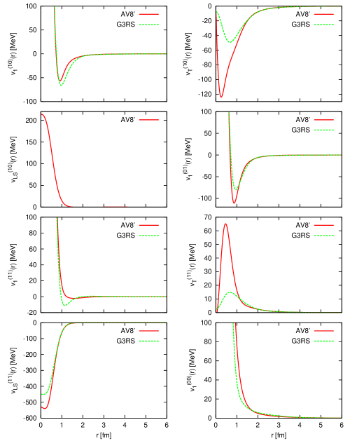
Figure 1: The nucleon-nucleon potentials of AV8^′ av8 and G3RS tamagaki .

The orbital part $\psi_{LM}^{(\rm space)}$ is given as follows

$$F_{(L_{1}L_{2})LM}(u_{1},u_{2},A,{\mbox{\boldmath$x$}})={\rm exp}\left(-{\frac{1}{2}}{\widetilde{{\mbox{\boldmath$x$}}}}A{\mbox{\boldmath$x$}}\right)[{\cal Y}_{L_{1}}({\widetilde{u_{1}}}{\mbox{\boldmath$x$}}){\cal Y}_{L_{2}}({\widetilde{u_{2}}}{\mbox{\boldmath$x$}})]_{LM},$$ (33)

with ${\cal Y}_{LM}({\mbox{\boldmath$r$}})=r^{L}Y_{LM}(\hat{\mbox{\boldmath$r$}})$, where ${\mbox{\boldmath$x$}}=({\mbox{\boldmath$x$}}_{1},{\mbox{\boldmath$x$}}_{2},\ldots,{\mbox{\boldmath$x$}}_{N-1})$ is a set of relative coordinates, say the Jacobi coordinate set, and $u_{1}$ and $u_{2}$ are $(N-1)$-dimensional column vectors which define the global vectors. Here ${\widetilde{{\mbox{\boldmath$x$}}}}A{\mbox{\boldmath$x$}}=\sum_{i,j=1}^{N-1}A_{ij}{\mbox{\boldmath$x$}}_{i}\cdot{\mbox{\boldmath$x$}}_{j}$ with $A_{ij}=A_{ji}$ and ${\widetilde{u_{1}}}{\mbox{\boldmath$x$}}=\sum_{i=1}^{N-1}{u_{1}}_{i}{\mbox{\boldmath$x$}}_{i}$. As we see, each basis function is characterized by a set of parameters, $A=(A_{ij})$, $u_{1}$, $u_{2}$, $L_{1},L_{2},L,S_{12},S_{123},\ldots,S,T_{12},T_{123},\ldots$.

The calculation of Hamiltonian matrix elements is made possible with the aid of the generating function $g$

$$g({\mbox{\boldmath$s$}};A,{\mbox{\boldmath$x$}})=\exp\Big{(}-{\frac{1}{2}}{\widetilde{\mbox{\boldmath$x$}}}A{\mbox{\boldmath$x$}}+\widetilde{\mbox{\boldmath$s$}}{\mbox{\boldmath$x$}}\Big{)},$$ (34)

where $s$ is an $(N-1)$-dimensional column vector whose $i$th element is a 3-dimensional vector ${\mbox{\boldmath$s$}}_{i}$. By expressing ${\mbox{\boldmath$s$}}_{i}$ with 3-dimensional unit vectors ${\mbox{\boldmath$e$}}_{1}$ and ${\mbox{\boldmath$e$}}_{2}$ as ${\mbox{\boldmath$s$}}_{i}={\lambda}_{1}{\mbox{\boldmath$e$}}_{1}u_{1_{i}}+{\lambda}_{2}{\mbox{\boldmath$e$}}_{2}u_{2_{i}}$, the basis function (33) is generated as follows:

$$F_{(L_{1}L_{2})LM}(u_{1},u_{2},A,{\mbox{\boldmath$x$}})={\frac{B_{L_{1}}B_{L_{2}}}{L_{1}!L_{2}!}}\int\!\int d{\mbox{\boldmath$e$}}_{1}\,d{\mbox{\boldmath$e$}}_{2}\,[Y_{L_{1}}({\mbox{\boldmath$e$}}_{1})Y_{L_{2}}({\mbox{\boldmath$e$}}_{2})]_{LM}$$

$$\qquad\qquad\qquad\qquad\times\,{\frac{\partial^{L_{1}+L_{2}}}{\partial{\lambda}_{1}^{L_{1}}\partial{\lambda}_{2}^{L_{2}}}}\,g({\lambda}_{1}{\mbox{\boldmath$e$}}_{1}u_{1}\!+\!{\lambda}_{2}{\mbox{\boldmath$e$}}_{2}u_{2};A,{\mbox{\boldmath$x$}})\Big{|}_{\lambda_{1}=\lambda_{2}=0},$$ (35)

where

$$B_{L}={\frac{(2L+1)!!}{4\pi}}.$$ (36)

Formulas for the matrix elements are given in Ref. fbs . In Appendix A we give a formula to calculate the $i$CF for the spin-orbit force, which was not included in Ref. fbs .

We study the $i$CF of $s$-shell nuclei, $d,\,t,\,h$, and ⁴He ($\alpha$). We also show the $i$CF calculated for the first excited $0^{+}$ state of ⁴He, which is called $\alpha^{*}$ in this paper. Although this state decays into the $t+p$ channel with a width of 0.50 MeV, approximating it as a bound state is fairly good, and the $i$CF of $\alpha^{*}$ are calculated using the wave function obtained in that approximation he4 . Because $\alpha^{*}$ is a spatially extended state with a cluster structure of $t+p$ and $h+n$, comparing the $i$CF between $\alpha^{*}$ and other cases reveals how much the shapes and magnitudes of the $i$CF are modified by the structures of the underlying nuclear states.

We use the AV8^′ potential av8 and the G3RS potential tamagaki as the two-nucleon interaction. Both of them contain central, tensor and spin-orbit terms. The ${\bm{L}}^{2}$ and $({\bm{L}\cdot{\bm{S}}})^{2}$ terms of the G3RS potential are ignored. The radial form factors $v^{(ST)}_{\cal O}$ of the two potentials are displayed in Fig. 1. As is well-known, the longest-range attraction of the two-nucleon interaction is that belonging to the $v_{\rm T}^{(10)}$ term. In the intermediate region $(1<r<1.6)$ fm, the singlet even central potential $v^{(01)}_{1}$ is most attractive, and then the $v_{\rm T}^{(10)}$ and $v_{1}^{(01)}$ terms follow. The central potentials all have strong short-range repulsion. Generally speaking, the G3RS potential is softer than the AV8^′ potential. The tensor force of the latter potential is much stronger at $r<1\,$fm than that of the G3RS potential. The G3RS potential has no $v_{\rm LS}^{(10)}$ component. In spite of these differences, the two potentials give rather similar binding energies for the $s$-shell nuclei fbs .

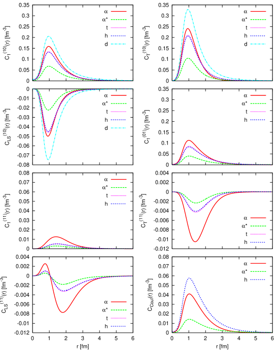
Figure 2: The $i$CF for $\alpha,\,\alpha^{*}$ (the first excited $0^{+}$ state of ⁴He), $t,\,h,\,d$ calculated using the AV8^′ potential. Note that different scales are used for the vertical axes.

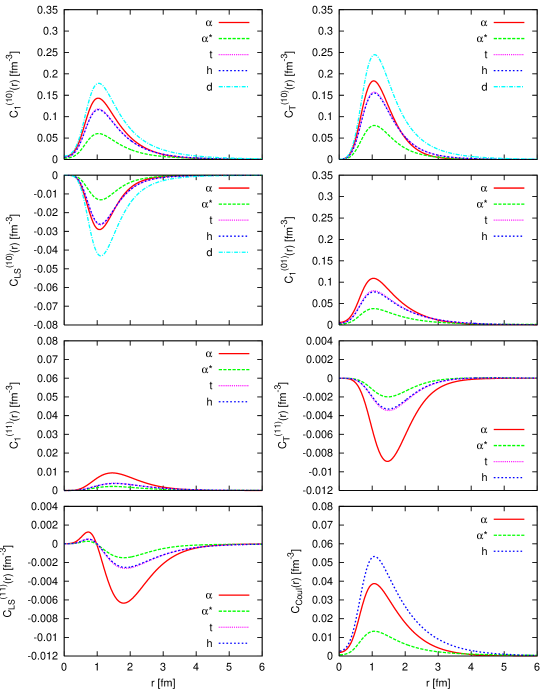
Figure 3: The same as Fig. 2 but calculated using the G3RS potential.

Figures 2 and 3 compare the $i$CF, $C^{(ST)}_{\cal O}(r)$, calculated using the wave functions obtained with the AV8^′ Hamiltonian with those obtained with the G3RS Hamiltonian. The amplitude of $C_{1}^{(00)}$ is by far smaller than the others because of the purely repulsive nature of the corresponding potential $v_{1}^{(00)}$, and thus it is not shown in the figures. Common to the two cases is that the three $i$CF, $C_{\rm T}^{(10)},\,C_{1}^{(10)}$ and $C_{1}^{(01)}$, among others have much larger amplitudes than the others, all having a peak at around 1 fm. This is understandable from the characteristics of the $v^{(ST)}_{\cal O}$ curves shown in Fig. 1. The more attractive the potential component, the larger the amplitude of the corresponding $i$CF. The central potential for even partial waves has a minimum around 1 fm. Since the central and tensor forces in the triplet even channels couple, the $C_{\rm T}^{(10)}$ curve also has a peak at almost the same position as that of $C_{1}^{(10)}$, though the $v_{\rm T}^{(10)}$ potential does not have a minimum around 1 fm. Both of $C_{1}^{(11)}$ and $C_{\rm T}^{(11)}$ curves have a peak around 1.4-1.5 fm because the central and tensor forces in the $(ST)=(11)$ channel couple and the central force has a shallow attraction beyond 1 fm. The peak position of the $i$CF for the Coulomb potential is the same as that of the main terms of the triplet even channel.

Because of the strong short-range repulsion of the central potentials $v_{1}^{(ST)}$, all the $C^{(ST)}_{\cal O}$ vanish near the origin. The spin-orbit force ($v^{(11)}_{\rm LS}$) has a very strong attraction around 1 fm but it is confined to the short distance region. Comparing Figs. 2 and 3, the difference of the $i$CF produced by the potential models is mild in spite of apparently different behaviors of the potential form factors, for example of the tensor terms.

The $s$-shell nuclei all produce similar shapes for each of the $i$CF. It is interesting to note the $i$CF of $\alpha^{*}$ exhibit the patterns similar to the other cases, despite the fact that its structure is quite different from that of $\alpha$. Of course the amplitudes at larger values of $r$ are much larger for $\alpha^{*}$ than for the other cases.

A remarkable characteristics of the $i$CF is that their asymptotics for a given nucleus are the same for all the $C^{(ST)}_{\cal O}$. For example, the eight $i$CF calculated for $\alpha$ using the AV8^′ potential follow $\sim\exp(-2\kappa r)/r^{2.09}$ with $\kappa=0.75$ fm^-1 for $r$ larger than 6 fm.

The case of the deuteron is easily understood. The deuteron wave function consists of the $S$- and $D$-wave components

$$\Psi=\phi_{0}(r)Y_{00}(\hat{\mbox{\boldmath$r$}})\chi_{1M}\eta_{00}+\phi_{2}(r)[Y_{2}(\hat{\mbox{\boldmath$r$}})\chi_{1}]_{1M}\eta_{00},$$ (37)

where $\chi_{1}$ and $\eta_{0}$ are the spin and isospin functions of the deuteron. For large values of $r$ for which the nuclear potential between the two nucleons in the deuteron are negligible, the Hamiltonian for the deuteron reduces to the kinetic energy alone, and thus the radial function $\phi_{\ell}(r)$ should be given by a solution of the free-particle Schrödinger equation with the negative energy ($-{\hbar^{2}\kappa^{2}}/m$) of the deuteron, that is the spherical Hankel function of the first kind $h_{\ell}^{(1)}(i\kappa r)$. The asymptotic form of the deuteron wave function is therefore given by

$$\Psi=\sum_{\ell=0,2}K_{\ell}h_{\ell}^{(1)}(i\kappa r)[Y_{\ell}(\hat{\mbox{\boldmath$r$}})\chi_{1}]_{1M}\eta_{00}$$ (38)

with suitable coefficients $K_{\ell}$. The $i$CF of the deuteron for large $r$ reduces to

$$C^{(ST)}_{\cal O}(r)\sim\sum_{\ell,\ell^{\prime}=0,2}K_{\ell}K^{*}_{\ell^{\prime}}\langle[Y_{\ell^{\prime}}\chi_{1}]_{1M}\eta_{00}|{\cal O}P^{(ST)}|[Y_{\ell}\chi_{1}]_{1M}\eta_{00}\rangle h_{\ell}^{(1)}(i\kappa r){h_{\ell^{\prime}}^{(1)}}^{*}(i\kappa r).$$ (39)

All of the $i$Cf for the deuteron displayed in Figs. 2 and 3 satisfy the above behavior for $r\geq 5\,$fm.

The asymptotic behavior for other cases is discussed in Appendix B by taking into account the Coulomb force. The case of $\alpha$ is understood by taking the nucleus R (in the notation of Appendix B) as the $pn$ system, which gives $Z=2$. See Eq. (63). As discussed in Appendix B, the asymptotic behavior is given by $r^{-2-2\eta}\exp(-2\kappa r)$, where $\eta$ defined in Eq. (65) becomes 0.046 for $\kappa=0.75$ fm^-1. Thus we can understand the asymptotic behavior of the $i$CF noted above.

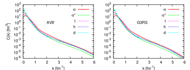
Figure 4: The $i$CF for the kinetic energy operator.

The $i$CF $C(k)$ for the kinetic energy operator is shown in Fig. 4. The AV8^′ and G3RS potentials give qualitatively very similar results. The behavior of $C(k)$ for small values of $k$ is given analytically as explained in Appendix B. The numerical results confirm that the asymptotic form, Eq. (70), agrees with $C(k)$ for small values of $k$. The behavior of $C(k)$ for large values of $k$ primarily reflects the short-range central correlation and the tensor correlation involved in the wave function. The enhancement of the curve around $k\sim 1.3$ fm^-1 is due to the tensor force, as shown in Ref. he6 .

Figure 5 displays the kinetic energy density of the two-nucleon relative motion, $(\hbar^{2}/m)k^{4}C(k)$, as a function of $k$. We clearly see that the tensor correlation increases the kinetic energy density beyond $k=1$ fm^-1. The height of the density around $k=1.5$ fm^-1 is related to the components of higher partial waves induced by the tensor force. The $\alpha$ particle contains the largest bump among the $s$-shell nuclei, but the component contained in the first excited $0^{+}$ state ($\alpha^{*}$) is much smaller as understood from the $3N+N$ cluster structure. The kinetic energy density extends beyond $k=6$ fm^-1 for all the nuclei, which is of course due to the short-range repulsion of the central interaction.

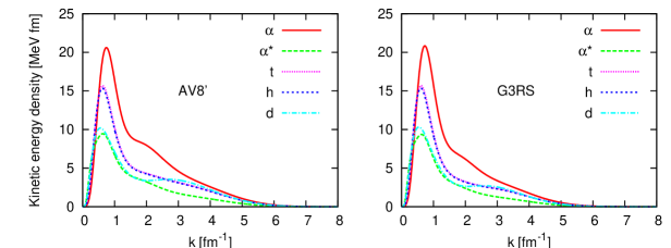
Figure 5: Two-nucleon relative kinetic energy density per unit wave number.

IV Summary

We have shown that the ground state energy of a nucleus as a self-bound system is a functional of a set of internucleon correlation functions including the kinetic energy term. Conversely the set of the internucleon correlation functions uniquely determines the nuclear Hamiltonian. Namely, there is a one-to-one correspondence between the nuclear Hamiltonian and the internucleon correlation functions. The ground state energy becomes a minimum for a set of the exact internucleon correlation functions.

Using the accurate wave functions for $s$-shell nuclei, we have calculated the internucleon correlation functions for $d,\,^{3}$H, ³He and the ground state of ⁴He. To see the dependence of the correlation functions on nuclear structure, we have also included the first excited $0^{+}$ state of ⁴He. We used two different potentials, AV8^′ and G3RS, as the two-nucleon interaction. Both of them contain central, tensor and spin-orbit components. We have shown that the magnitude and the shape of each of the internucleon correlation functions is clearly understood from the characteristics of the underlying two-nucleon interaction. The correlation function for the two-nucleon relative kinetic energy also indicates the importance of the tensor correlation and the short-range central repulsion in its momentum dependence.

We have discussed the asymptotic behavior of the internucleon correlation functions. For a large separation of the two nucleons, the correlation functions are determined by negative energy solutions of three-body systems interacting via Coulomb potentials.

Studying the internucleon correlation functions for heavier nuclei will be interesting and important because they give us direct information on the distribution of the internucleon motion. We expect that the shapes of the functions do not differ drastically from those in the lightest nuclei, but the heights of the peaks are expected to be smaller, and the larger the mass number, the larger the spatial extension of the correlation function.

Appendix A Correlation function for spin-orbit force

In this appendix we show a method of calculating the $i$CF for the spin-orbit force following the formulation of Ref. fbs . We use the notation used there to be consistent with the formulation, so that a reader is referred to Ref. fbs for details. Since the matrix elements of the spin and isospin parts are calculated using a standard method, we here focus on the spatial part only.

The spatial part of the spin-orbit force has the form $V(|{\mbox{\boldmath$r$}}_{ij}|)({\mbox{\boldmath$r$}}_{ij}\times{\mbox{\boldmath$\pi$}}_{ij})$. We can express ${\mbox{\boldmath$r$}}_{ij}={\mbox{\boldmath$r$}}_{i}-{\mbox{\boldmath$r$}}_{j}$ in terms of a linear combination of the relative coordinates ${\mbox{\boldmath$x$}}_{k}$, that is ${\mbox{\boldmath$r$}}_{ij}=\sum_{k=1}^{N-1}w_{k}{\mbox{\boldmath$x$}}_{k}=\widetilde{w}{\mbox{\boldmath$x$}}$. Similarly ${\mbox{\boldmath$\pi$}}_{ij}$ is expressed as ${\mbox{\boldmath$\pi$}}_{ij}=\sum_{k=1}^{N-1}\xi_{k}{\mbox{\boldmath$\pi$}}_{k}=\widetilde{\xi}{\mbox{\boldmath$\pi$}}$, where ${\mbox{\boldmath$\pi$}}_{k}=-i\partial/\partial{\mbox{\boldmath$x$}}_{k}$ is a momentum operator conjugate to ${\mbox{\boldmath$x$}}_{k}$. Thus the spin-orbit force $V(|{\mbox{\boldmath$r$}}_{ij}|)({\mbox{\boldmath$r$}}_{ij}\times{\mbox{\boldmath$\pi$}}_{ij})$ is expressed as $V(|\widetilde{w}{\mbox{\boldmath$x$}}|)(\widetilde{w}{\mbox{\boldmath$x$}}\times\widetilde{\xi}{\mbox{\boldmath$\pi$}})$.

The spin-orbit matrix element is calculated from the following expression

$$\langle F_{(L_{3}L_{4})L^{\prime}M^{\prime}}({u_{3}},{u_{4}},A^{\prime},{\mbox{\boldmath$x$}})|V(|\widetilde{w}{\mbox{\boldmath$x$}}|)(\widetilde{w}{\mbox{\boldmath$x$}}\times\widetilde{\xi}{\mbox{\boldmath$\pi$}})_{m}|F_{(L_{1}L_{2})LM}(u_{1},u_{2},A,{\mbox{\boldmath$x$}})\rangle$$

$$=\!\left(\prod_{i=1}^{4}{\frac{B_{L_{i}}}{L_{i}!}}\int d{\mbox{\boldmath$e$}}_{i}\right)([Y_{L_{3}}({\mbox{\boldmath$e$}}_{3})Y_{L_{4}}({\mbox{\boldmath$e$}}_{4})]_{L^{\prime}M^{\prime}})^{*}[Y_{L_{1}}({\mbox{\boldmath$e$}}_{1})Y_{L_{2}}({\mbox{\boldmath$e$}}_{2})]_{LM}\left(\prod_{i=1}^{4}{\frac{\partial^{L_{i}}}{\partial{{\lambda}_{i}}^{L_{i}}}}\right)$$

$$\,\times\,\langle g({\lambda}_{3}{\mbox{\boldmath$e$}}_{3}u_{3}\!+\!{\lambda}_{4}{\mbox{\boldmath$e$}}_{4}u_{4};A^{\prime},{\mbox{\boldmath$x$}})|V(|\widetilde{w}{\mbox{\boldmath$x$}}|)(\widetilde{w}{\mbox{\boldmath$x$}}\times\widetilde{\xi}{\mbox{\boldmath$\pi$}})_{m}|g({\lambda}_{1}{\mbox{\boldmath$e$}}_{1}u_{1}\!+\!{\lambda}_{2}{\mbox{\boldmath$e$}}_{2}u_{2};A,{\mbox{\boldmath$x$}})\rangle\Big{|}_{\lambda_{i}=0},$$ (40)

where $({\mbox{\boldmath$a$}}\times{\mbox{\boldmath$b$}})_{m}$ stands for $-\sqrt{2}i[{\mbox{\boldmath$a$}}\times{\mbox{\boldmath$b$}}]_{1m}\!=\!-(4\sqrt{2}\pi/3)iab[Y_{1}(\hat{\mbox{\boldmath$a$}})Y_{1}(\hat{\mbox{\boldmath$b$}})]_{1m}$. To calculate the spin-orbit matrix element between the generating functions, we make use of the relation

$$\langle g({\lambda}_{3}{\mbox{\boldmath$e$}}_{3}u_{3}\!+\!{\lambda}_{4}{\mbox{\boldmath$e$}}_{4}u_{4};A^{\prime},{\mbox{\boldmath$x$}})|V(|\widetilde{w}{\mbox{\boldmath$x$}}|)(\widetilde{w}{\mbox{\boldmath$x$}}\times\widetilde{\xi}{\mbox{\boldmath$\pi$}})_{m}|g({\lambda}_{1}{\mbox{\boldmath$e$}}_{1}u_{1}\!+\!{\lambda}_{2}{\mbox{\boldmath$e$}}_{2}u_{2};A,{\mbox{\boldmath$x$}})\rangle$$

$$= \int d{\mbox{\boldmath$r$}}\,V(r)\langle g({\lambda}_{3}u_{3}\!+\!{\lambda}_{4}{\mbox{\boldmath$e$}}_{4}u_{4};A^{\prime},{\mbox{\boldmath$x$}})|\delta(\widetilde{w}{\mbox{\boldmath$x$}}-{\mbox{\boldmath$r$}})(\widetilde{w}{\mbox{\boldmath$x$}}\times\widetilde{\xi}{\mbox{\boldmath$\pi$}})_{m}|g({\lambda}_{1}{\mbox{\boldmath$e$}}_{1}u_{1}\!+\!{\lambda}_{2}{\mbox{\boldmath$e$}}_{2}u_{2};A,{\mbox{\boldmath$x$}})\rangle,$$

with

$$\langle g({\lambda}_{3}{\mbox{\boldmath$e$}}_{3}u_{3}\!+\!{\lambda}_{4}{\mbox{\boldmath$e$}}_{4}u_{4};A^{\prime},{\mbox{\boldmath$x$}})|\delta(\widetilde{w}{\mbox{\boldmath$x$}}-{\mbox{\boldmath$r$}})(\widetilde{w}{\mbox{\boldmath$x$}}\times\widetilde{\xi}{\mbox{\boldmath$\pi$}})|g({\lambda}_{1}{\mbox{\boldmath$e$}}_{1}u_{1}\!+\!{\lambda}_{2}{\mbox{\boldmath$e$}}_{2}u_{2};A,{\mbox{\boldmath$x$}})\rangle$$

$$\quad=-i\left({\frac{(2\pi)^{N-2}c}{{\rm det}B}}\right)^{\frac{3}{2}}{\mbox{\boldmath$r$}}\times(\widetilde{\xi}{\mbox{\boldmath$z$}}\!+\!c\widetilde{\xi}AB^{-1}w\widetilde{w}B^{-1}{\mbox{\boldmath$v$}})$$

$$\quad\,\times\,{\rm exp}\left({\frac{1}{2}}\widetilde{\mbox{\boldmath$v$}}B^{-1}{\mbox{\boldmath$v$}}\!-\!{\frac{1}{2}}c({\mbox{\boldmath$r$}}\!-\!\widetilde{w}B^{-1}{\mbox{\boldmath$v$}})^{2}\right),$$ (42)

where $B=A+A^{\prime}$, $c=(\widetilde{w}B^{-1}w)^{-1}$, and ${\mbox{\boldmath$z$}}=\sum_{i=1}^{4}\lambda_{i}{\mbox{\boldmath$e$}}_{i}A_{i}B^{-1}$ with $A_{1}=A_{2}=A^{\prime},\,A_{3}=A_{4}=-A$. When the radial form of the spin-orbit potential is scalar, i.e. $V$ is a function of $r$, we may omit $c\widetilde{\xi}AB^{-1}w\widetilde{w}B^{-1}{\mbox{\boldmath$v$}}$ thanks to the relation

$$\int d{\mbox{\boldmath$r$}}\,V(r)({\mbox{\boldmath$r$}}\times{\mbox{\boldmath$a$}})\,{\rm exp}\left(-{\frac{1}{2}}c({\mbox{\boldmath$r$}}-{\mbox{\boldmath$a$}})^{2}\right)=0,$$ (43)

which leads to

$$\langle g({\lambda}_{3}{\mbox{\boldmath$e$}}_{3}u_{3}\!+\!{\lambda}_{4}{\mbox{\boldmath$e$}}_{4}u_{4};A^{\prime},{\mbox{\boldmath$x$}})|V(|\widetilde{w}{\mbox{\boldmath$x$}}|)(\widetilde{w}{\mbox{\boldmath$x$}}\times\widetilde{\xi}{\mbox{\boldmath$\pi$}})_{m}|g({\lambda}_{1}{\mbox{\boldmath$e$}}_{1}u_{1}\!+\!{\lambda}_{2}{\mbox{\boldmath$e$}}_{2}u_{2};A,{\mbox{\boldmath$x$}})\rangle$$

$$\longrightarrow-i\left({\frac{(2\pi)^{N-2}c}{{\rm det}B}}\right)^{\frac{3}{2}}\int d{\mbox{\boldmath$r$}}\,V(r)({\mbox{\boldmath$r$}}\times\widetilde{\xi}{\mbox{\boldmath$z$}})_{m}$$

$$\qquad\times{\rm exp}\left(-{\frac{1}{2}}cr^{2}+\sum_{j>i=1}^{4}\bar{\rho}_{ij}\lambda_{i}\lambda_{j}{\mbox{\boldmath$e$}}_{i}\cdot{\mbox{\boldmath$e$}}_{j}+c\sum_{i=1}^{4}\gamma_{i}\lambda_{i}{\mbox{\boldmath$e$}}_{i}\cdot{\mbox{\boldmath$r$}}\right),$$ (44)

where $\gamma_{i}=\widetilde{w}B^{-1}u_{i}$, $\bar{\rho}_{ij}=\widetilde{u_{i}}B^{-1}u_{j}-c\gamma_{i}\gamma_{j}$, and we set

$$({\mbox{\boldmath$r$}}\times\widetilde{\xi}{\mbox{\boldmath$z$}})_{m}=-\sqrt{2}i\sum_{\alpha=1}^{4}T_{\alpha}\lambda_{\alpha}[{\mbox{\boldmath$r$}}\times{\mbox{\boldmath$e$}}_{\alpha}]_{1m}$$ (45)

with

$$T_{\alpha}=\widetilde{\xi}A_{\alpha}B^{-1}u_{\alpha}.$$ (46)

The symbol $\longrightarrow$ in Eq. (44) indicates that the $\lambda_{i}^{2}$ terms in the exponent, which give no contribution to the required matrix element, are dropped. See Ref. fbs for details. Substitution of Eqs. (44) and (45) into Eq. (40) yields a basic equation to obtain the spin-orbit matrix element

$$\langle F_{(L_{3}L_{4})L^{\prime}M^{\prime}}({u_{3}},{u_{4}},A^{\prime},{\mbox{\boldmath$x$}})|V(|\widetilde{w}{\mbox{\boldmath$x$}}|)(\widetilde{w}{\mbox{\boldmath$x$}}\times\widetilde{\xi}{\mbox{\boldmath$\pi$}})_{m}|F_{(L_{1}L_{2})LM}(u_{1},u_{2},A,{\mbox{\boldmath$x$}})\rangle$$

$$=-\sqrt{2}\left({\frac{(2\pi)^{N-2}c}{{\rm det}B}}\right)^{\frac{3}{2}}\sum_{\alpha=1}^{4}T_{\alpha}\int d{\mbox{\boldmath$r$}}\,V(r)\,{\rm e}^{-\frac{1}{2}cr^{2}}$$

$$\,\times\prod_{i=1}^{4}\left({\frac{B_{L_{i}}}{L_{i}!}}\int d{\mbox{\boldmath$e$}}_{i}\right)([Y_{L_{3}}({\mbox{\boldmath$e$}}_{3})Y_{L_{4}}({\mbox{\boldmath$e$}}_{4})]_{L^{\prime}M^{\prime}})^{*}[Y_{L_{1}}({\mbox{\boldmath$e$}}_{1})Y_{L_{2}}({\mbox{\boldmath$e$}}_{2})]_{LM}$$

$$\,\times\,{\frac{\partial^{L_{i}}}{\partial{{\lambda}_{i}}^{L_{i}}}}\lambda_{\alpha}[{\mbox{\boldmath$r$}}\times{\mbox{\boldmath$e$}}_{\alpha}]_{1m}\,{\rm exp}\left(\sum_{j>i=1}^{4}\bar{\rho}_{ij}\lambda_{i}\lambda_{j}{\mbox{\boldmath$e$}}_{i}\cdot{\mbox{\boldmath$e$}}_{j}+c\sum_{i=1}^{4}\gamma_{i}\lambda_{i}{\mbox{\boldmath$e$}}_{i}\cdot{\mbox{\boldmath$r$}}\right)\Big{|}_{\lambda_{i}=0}.$$ (47)

We now have three expressions depending on ${\mbox{\boldmath$e$}}_{i}$, two in the exponent and one in $\lambda_{\alpha}[{\mbox{\boldmath$r$}}\times{\mbox{\boldmath$e$}}_{\alpha}]_{1m}$. Using the formula (B.4) of Ref. fbs , we can rewrite the first expression as

$${\rm exp}\left(\sum_{j>i=1}^{4}\bar{\rho}_{ij}\lambda_{i}\lambda_{j}{\mbox{\boldmath$e$}}_{i}\cdot{\mbox{\boldmath$e$}}_{j}\right)$$

$$\Rightarrow\sum_{p_{ij}}\left(\prod_{j>i=1}^{4}\frac{(-1)^{p_{ij}}\sqrt{2p_{ij}+1}}{B_{p_{ij}}}(\bar{\rho}_{ij})^{p_{ij}}\right)\sum_{\kappa}X(p_{13}p_{14}p_{23}p_{24};\kappa)$$

$$\quad\times\,Y(p_{12}p_{12}p_{34}p_{34}\,p_{13}\!+\!p_{14}\,p_{23}\!+\!p_{24}\,p_{13}\!+\!p_{23}\,p_{14}\!+\!p_{24}\,0\kappa\kappa 0;\kappa\kappa)$$

$$\quad\times\,\Big{[}\big{[}Y_{p_{12}+p_{13}+p_{14}}({\mbox{\boldmath$e$}}_{1})Y_{p_{12}+p_{23}+p_{24}}({\mbox{\boldmath$e$}}_{2})\big{]}_{\kappa}\big{[}Y_{p_{13}+p_{23}+p_{34}}({\mbox{\boldmath$e$}}_{3})Y_{p_{14}+p_{24}+p_{34}}({\mbox{\boldmath$e$}}_{4})\big{]}_{\kappa}\Big{]}_{00}$$

$$\quad\times\,\lambda_{1}^{p_{12}+p_{13}+p_{14}}\lambda_{2}^{p_{12}+p_{23}+p_{24}}\lambda_{3}^{p_{13}+p_{23}+p_{34}}\lambda_{4}^{p_{14}+p_{24}+p_{34}}.$$ (48)

The symbol $\Rightarrow$ indicates that the angular momentum coupling must be made to its maximum value for each ${\mbox{\boldmath$e$}}_{i}$. See Ref. fbs for details. The coefficients $X$ and $Y$ are defined in Eqs. (B.7) and (B.9) of Ref. fbs . With the use of Eq. (B.22) of Ref. fbs , the second term reduces to

$${\rm exp}\left(c\sum_{i=1}^{4}\gamma_{i}\lambda_{i}{\mbox{\boldmath$e$}}_{i}\cdot{\mbox{\boldmath$r$}}\right)$$

$$\Rightarrow\sum_{q_{i}}\left(\prod_{i=1}^{4}\frac{(-1)^{q_{i}}(c\gamma_{i})^{q_{i}}}{B_{q_{i}}}r^{q_{i}}\right)\sum_{\mu\mu^{\prime}\ell}\sqrt{2\ell+1}\,C(q_{1}q_{2};\mu)\,C(q_{3}q_{4};\mu^{\prime})\,C(\mu\mu^{\prime};\ell)$$

$$\quad\times\,\Big{[}\big{[}[Y_{q_{1}}({\mbox{\boldmath$e$}}_{1})Y_{q_{2}}({\mbox{\boldmath$e$}}_{2})]_{\mu}[Y_{q_{3}}({\mbox{\boldmath$e$}}_{3})Y_{q_{4}}({\mbox{\boldmath$e$}}_{4})]_{\mu^{\prime}}\big{]}_{\ell}Y_{\ell}(\hat{\mbox{\boldmath$r$}})\Big{]}_{00}\lambda_{1}^{q_{1}}\lambda_{2}^{q_{2}}\lambda_{3}^{q_{3}}\lambda_{4}^{q_{4}}.$$ (49)

Here $C$ is a coefficient which couples two spherical harmonics with the same argument

$$C(l_{1}l_{2};l_{3})=\sqrt{\frac{(2l_{1}\!+\!1)(2l_{2}\!+\!1)}{4\pi(2l_{3}\!+\!1)}}\langle l_{1}0l_{2}0|l_{3}0\rangle.$$ (50)

Note that $\ell$ in the above summation (49) must be 1 to get a nonvanishing contribution in Eq. (47) because the term $\lambda_{\alpha}[{\mbox{\boldmath$r$}}\times{\mbox{\boldmath$e$}}_{\alpha}]_{1m}$ behaves like a vector in $r$, which is simply given as

$$\lambda_{\alpha}[{\mbox{\boldmath$r$}}\times{\mbox{\boldmath$e$}}_{\alpha}]_{1m}=-\frac{4\pi}{3}r[Y_{1}({\mbox{\boldmath$e$}}_{\alpha})Y_{1}(\hat{\mbox{\boldmath$r$}})]_{1m}\lambda_{\alpha}.$$ (51)

From Eqs. (49) and (51) we have

$$\Big{[}\big{[}[Y_{q_{1}}({\mbox{\boldmath$e$}}_{1})Y_{q_{2}}({\mbox{\boldmath$e$}}_{2})]_{\mu}[Y_{q_{3}}({\mbox{\boldmath$e$}}_{3})Y_{q_{4}}({\mbox{\boldmath$e$}}_{4})]_{\mu^{\prime}}\big{]}_{1}Y_{1}(\hat{\mbox{\boldmath$r$}})\Big{]}_{00}\lambda_{1}^{q_{1}}\lambda_{2}^{q_{2}}\lambda_{3}^{q_{3}}\lambda_{4}^{q_{4}}[Y_{1}({\mbox{\boldmath$e$}}_{\alpha})Y_{1}(\hat{\mbox{\boldmath$r$}})]_{1m}\lambda_{\alpha}$$

$$\Rightarrow\frac{1}{4\sqrt{3}\pi}\Big{[}\big{[}[Y_{q_{1}}({\mbox{\boldmath$e$}}_{1})Y_{q_{2}}({\mbox{\boldmath$e$}}_{2})]_{\mu}[Y_{q_{3}}({\mbox{\boldmath$e$}}_{3})Y_{q_{4}}({\mbox{\boldmath$e$}}_{4})]_{\mu^{\prime}}\big{]}_{1}Y_{1}({\mbox{\boldmath$e$}}_{\alpha})\Big{]}_{1m}\lambda_{1}^{q_{1}}\lambda_{2}^{q_{2}}\lambda_{3}^{q_{3}}\lambda_{4}^{q_{4}}\lambda_{\alpha},$$ (52)

where the two $Y_{1}(\hat{\mbox{\boldmath$r$}})$’s are coupled to a scalar. Note that the integration over $\hat{\mbox{\boldmath$r$}}$ in Eq. (47) gives $4\pi$. It is convenient to express Eq. (52) as

$$\Big{[}\big{[}[Y_{q_{1}}({\mbox{\boldmath$e$}}_{1})Y_{q_{2}}({\mbox{\boldmath$e$}}_{2})]_{\mu}[Y_{q_{3}}({\mbox{\boldmath$e$}}_{3})Y_{q_{4}}({\mbox{\boldmath$e$}}_{4})]_{\mu^{\prime}}\big{]}_{1}Y_{1}({\mbox{\boldmath$e$}}_{\alpha})\Big{]}_{1m}\lambda_{1}^{q_{1}}\lambda_{2}^{q_{2}}\lambda_{3}^{q_{3}}\lambda_{4}^{q_{4}}\lambda_{\alpha}$$

$$\Rightarrow\sum_{\nu\nu^{\prime}}K_{\alpha}(q_{1}q_{2}q_{3}q_{4}\mu\mu^{\prime};\nu\nu^{\prime})$$

$$\quad\times\big{[}[Y_{q_{1\alpha}}({\mbox{\boldmath$e$}}_{1})Y_{q_{2\alpha}}({\mbox{\boldmath$e$}}_{2})]_{\nu}[Y_{q_{3\alpha}}({\mbox{\boldmath$e$}}_{3})Y_{q_{4\alpha}}({\mbox{\boldmath$e$}}_{4})]_{\nu^{\prime}}\big{]}_{1m}\lambda_{1}^{q_{1\alpha}}\lambda_{2}^{q_{2\alpha}}\lambda_{3}^{q_{3\alpha}}\lambda_{4}^{q_{4\alpha}},$$ (53)

where

$$q_{i\alpha}=q_{i}+\delta_{i\alpha}.$$ (54)

An expression for the coefficient $K_{\alpha}$ will be given later. The coupling of Eqs. (48) and (53) must lead to $\big{[}[Y_{L_{1}}({\mbox{\boldmath$e$}}_{1})Y_{L_{2}}({\mbox{\boldmath$e$}}_{2})]_{L}[Y_{L_{3}}({\mbox{\boldmath$e$}}_{3})Y_{L_{4}}({\mbox{\boldmath$e$}}_{4})]_{L^{\prime}}\big{]}_{1m}$ in order to have a nonvanishing contribution in Eq. (47). This coupling gives the following factor

$$\Big{[}\big{[}Y_{p_{12}+p_{13}+p_{14}}({\mbox{\boldmath$e$}}_{1})Y_{p_{12}+p_{23}+p_{24}}({\mbox{\boldmath$e$}}_{2})\big{]}_{\kappa}\big{[}Y_{p_{13}+p_{23}+p_{34}}({\mbox{\boldmath$e$}}_{3})Y_{p_{14}+p_{24}+p_{34}}({\mbox{\boldmath$e$}}_{4})\big{]}_{\kappa}\Big{]}_{00}$$

$$\,\times\big{[}[Y_{q_{1\alpha}}({\mbox{\boldmath$e$}}_{1})Y_{q_{2\alpha}}({\mbox{\boldmath$e$}}_{2})]_{\nu}[Y_{q_{3\alpha}}({\mbox{\boldmath$e$}}_{3})Y_{q_{4\alpha}}({\mbox{\boldmath$e$}}_{4})]_{\nu^{\prime}}\big{]}_{1m}$$

$$\Rightarrow Y(p_{12}\!+\!p_{13}\!+\!p_{14}\,p_{12}\!+\!p_{23}\!+\!p_{24}\,p_{13}\!+\!p_{23}\!+\!p_{34}\,p_{14}\!+\!p_{24}\!+\!p_{34}\,q_{1\alpha}q_{2\alpha}q_{3\alpha}q_{4\alpha}\,\kappa\nu\nu^{\prime}1;LL^{\prime})$$

$$\quad\times\big{[}[Y_{L_{1}}({\mbox{\boldmath$e$}}_{1})Y_{L_{2}}({\mbox{\boldmath$e$}}_{2})]_{L}[Y_{L_{3}}({\mbox{\boldmath$e$}}_{3})Y_{L_{4}}({\mbox{\boldmath$e$}}_{4})]_{L^{\prime}}\big{]}_{1m}.$$ (55)

The values of $p_{ij}$ and $q_{i}$ must satisfy the following equations:

$$p_{12}+p_{13}+p_{14}+q_{1\alpha}=L_{1},\ \ \ p_{12}+p_{23}+p_{24}+q_{2\alpha}=L_{2},$$

$$p_{13}+p_{23}+p_{34}+q_{3\alpha}=L_{3},\ \ \ p_{14}+p_{24}+p_{34}+q_{4\alpha}=L_{4}.$$ (56)

The operation prescribed in Eq. (47) is now easily performed.

To sum up these results, we obtain the following formula:

$$\langle F_{(L_{3}L_{4})L^{\prime}M^{\prime}}({u_{3}},{u_{4}},A^{\prime},{\mbox{\boldmath$x$}})|V(|\widetilde{w}{\mbox{\boldmath$x$}}|)(\widetilde{w}{\mbox{\boldmath$x$}}\times\widetilde{\xi}{\mbox{\boldmath$\pi$}})_{m}|F_{(L_{1}L_{2})LM}(u_{1},u_{2},A,{\mbox{\boldmath$x$}})\rangle$$

$$=4\pi\sqrt{\frac{2}{3}}\frac{(-1)^{L_{1}+L_{2}+L+L^{\prime}+1}}{\sqrt{2L^{\prime}+1}}\langle LM1m|L^{\prime}M^{\prime}\rangle\left(\prod_{i=1}^{4}B_{L_{i}}\right)\left({\frac{(2\pi)^{N-2}c}{{\rm det}B}}\right)^{\frac{3}{2}}$$

$$\quad\times\sum_{\alpha=1}^{4}T_{\alpha}\sum_{p_{ij}}\left(\prod_{j>i=1}^{4}\frac{(-1)^{p_{ij}}\sqrt{2p_{ij}+1}}{B_{p_{ij}}}(\bar{\rho}_{ij})^{p_{ij}}\right)\sum_{\kappa}X(p_{13}p_{14}p_{23}p_{24};\kappa)$$

$$\quad\times\,Y(p_{12}p_{12}p_{34}p_{34}\,p_{13}\!+\!p_{14}\,p_{23}\!+\!p_{24}\,p_{13}\!+\!p_{23}\,p_{14}\!+\!p_{24}\,0\kappa\kappa 0;\kappa\kappa)$$

$$\quad\times\sum_{q_{i}}\left(\prod_{i=1}^{4}\frac{(-1)^{q_{i}}(c\gamma_{i})^{q_{i}}}{B_{q_{i}}}\right)\sum_{\mu\mu^{\prime}}\,C(q_{1}q_{2};\mu)\,C(q_{3}q_{4};\mu^{\prime})\,C(\mu\mu^{\prime};1)$$

$$\quad\times\int_{0}^{\infty}d{r}\,r^{q_{1}+q_{2}+q_{3}+q_{4}+3}\,{\rm e}^{-\frac{1}{2}cr^{2}}\,V(r)\sum_{\nu\nu^{\prime}}K_{\alpha}(q_{1}q_{2}q_{3}q_{4}\mu\mu^{\prime};\nu\nu^{\prime})$$

$$\quad\times Y(L_{1}\!-\!q_{1\alpha}\,L_{2}\!-\!q_{2\alpha}\,L_{3}\!-\!q_{3\alpha}\,L_{4}\!-\!q_{4\alpha}\,q_{1\alpha}q_{2\alpha}q_{3\alpha}q_{4\alpha}\,\kappa\nu\nu^{\prime}1;LL^{\prime}).$$ (57)

The coefficients $K_{\alpha}$ are given as follows:

$$K_{1}(q_{1}q_{2}q_{3}q_{4}\mu\mu^{\prime};\nu\nu^{\prime})=-\delta_{\nu^{\prime}\mu^{\prime}}C(q_{1}1;q_{11})U(\mu^{\prime}\mu 11;1\nu)U(q_{2}q_{1}\nu 1;\mu q_{11}),$$

$$K_{2}(q_{1}q_{2}q_{3}q_{4}\mu\mu^{\prime};\nu\nu^{\prime})=(-)^{\mu+\nu}\delta_{\nu^{\prime}\mu^{\prime}}C(q_{2}1;q_{22})U(\mu^{\prime}\mu 11;1\nu)U(q_{1}q_{2}\nu 1;\mu q_{22}),$$

$$K_{3}(q_{1}q_{2}q_{3}q_{4}\mu\mu^{\prime};\nu\nu^{\prime})=(-)^{\mu^{\prime}+\nu^{\prime}+1}\delta_{\nu\mu}C(q_{3}1;q_{33})U(\mu\mu^{\prime}11;1\nu^{\prime})U(q_{4}q_{3}\nu^{\prime}1;\mu^{\prime}q_{33}),$$

$$K_{4}(q_{1}q_{2}q_{3}q_{4}\mu\mu^{\prime};\nu\nu^{\prime})=\delta_{\nu\mu}C(q_{4}1;q_{44})U(\mu\mu^{\prime}11;1\nu^{\prime})U(q_{3}q_{4}\nu^{\prime}1;\mu^{\prime}q_{44}).$$ (58)

The values of $\nu$ and $\nu^{\prime}$ are constrained by triangular relations which come from the unitary Racah coefficients $U$. Choosing $V(|\widetilde{w}{\mbox{\boldmath$x$}}|)=\delta(|\widetilde{w}{\mbox{\boldmath$x$}}|-r)/r^{2}$ in Eq. (57) leads to the $i$CF for the spin-orbit force.

Appendix B Asymptotics of internucleon correlation functions

Here we discuss the asymptotic form of the $i$CF. Let ${\mbox{\boldmath$x$}}_{1}$ (instead of ${\mbox{\boldmath$r$}}_{12}$) denote the relative distance vector of nucleons 1 and 2, and ${\mbox{\boldmath$x$}}_{2}$ denote the coordinate of their center of mass relative to the center of mass of the rest of the nucleus, which is called a nucleus R, containing $N-2$ nucleons. When two nucleons are separated far in distance from R, all the nuclear forces can be neglected, and only the Coulomb interactions among them remain. The Hamiltonian $H$ of the whole system thus reduces to

$$t_{1}+t_{2}+\frac{e^{2}}{x_{1}}P_{1\pi}P_{2\pi}+\frac{Z_{R}e^{2}}{|\frac{1}{2}{\mbox{\boldmath$x$}}_{1}+{\mbox{\boldmath$x$}}_{2}|}P_{1\pi}+\frac{Z_{R}e^{2}}{|-\frac{1}{2}{\mbox{\boldmath$x$}}_{1}+{\mbox{\boldmath$x$}}_{2}|}P_{2\pi}+H_{R},$$ (59)

where $t_{1}$ and $t_{2}$ are the kinetic energies, $t_{1}=-(\hbar^{2}/m)\partial^{2}/\partial{\mbox{\boldmath$x$}}_{1}^{2}$, and $t_{2}=-(\hbar^{2}/2\mu)\partial^{2}/\partial{\mbox{\boldmath$x$}}_{2}^{2}$ with $\mu=2(N-2)m/N$. The charge of the nucleus R is $Z_{R}e$, and its internal Hamiltonian is denoted by $H_{R}$. Corresponding to this decomposition, the wave function $\Psi$ for large $x_{1}$ takes the form

$$\Psi=\sum_{LS_{12}T_{12}IJ_{R}T_{R}}K_{LS_{12}T_{12}IJ_{R}T_{R}}[[\Phi_{L}({\mbox{\boldmath$x$}}_{1},{\mbox{\boldmath$x$}}_{2})\chi_{S_{12}}]_{I}\eta_{T_{12}}\Psi_{J_{R}T_{R}}]_{JM_{J}TM_{T}},$$ (60)

where $\Psi_{J_{R}T_{R}}$ is the normalized wave function of R with spin $J_{R}$ and isospin $T_{R}$, though it may not be always an eigenstate of $H_{R}$. Let $E_{J_{R}T_{R}}$ be the energy expectation value which $\Psi_{J_{R}T_{R}}$ gives, $\langle\Psi_{J_{R}T_{R}}|H_{R}|\Psi_{J_{R}T_{R}}\rangle$. The spin and isospin states of nucleons 1 and 2 are represented by $\chi_{S_{12}}$ and $\eta_{T_{12}}$. The summation labels of Eq. (60) run over all possible angular momenta which satisfy the angular momentum couplings and the parity conservation as well as the Fermi statistics of nucleons 1 and 2.

Using the asymptotic forms, (59) and (60), in $H\Psi=E\Psi$, we find that the wave function $\Phi_{L}$ satisfies the three-body equation with only Coulomb potentials

$$\left(t_{1}+t_{2}+\frac{e^{2}}{x_{1}}P_{1\pi}P_{2\pi}+\frac{Z_{R}e^{2}}{|\frac{1}{2}{\mbox{\boldmath$x$}}_{1}+{\mbox{\boldmath$x$}}_{2}|}P_{1\pi}+\frac{Z_{R}e^{2}}{|-\frac{1}{2}{\mbox{\boldmath$x$}}_{1}+{\mbox{\boldmath$x$}}_{2}|}P_{2\pi}\right)\Phi_{LM_{L}}=(E-E_{J_{R}T_{R}})\Phi_{LM_{L}}.$$ (61)

The energy $E-E_{J_{R}T_{R}}$ is however negative in contrast to a usual case papp . Since $\Psi$ is a bound state wave function, $\Phi_{LM_{L}}$ must also be bound. A solution for large $x_{1}$ can be obtained by solving the above equation. Here we attempt to obtain an approximate solution by taking the leading term of the nucleon-R Coulomb potential.

Assuming that $x_{1}$ is much larger than $x_{2}$ makes it possible to simplify Eq. (61) to

$$\left(t_{1}+t_{2}+\frac{Ze^{2}}{x_{1}}\right)\Phi_{LM_{L}}=(E-E_{J_{R}T_{R}})\Phi_{LM_{L}},$$ (62)

with

$$Z=P_{1\pi}P_{2\pi}+2Z_{R}(P_{1\pi}+P_{2\pi}).$$ (63)

Since the coordinates ${\mbox{\boldmath$x$}}_{1}$ and ${\mbox{\boldmath$x$}}_{2}$ are now decoupled, we find a solution of the type of $\Phi_{LM_{L}}=[\psi_{\ell}({\mbox{\boldmath$x$}}_{1})\phi_{\lambda}({\mbox{\boldmath$x$}}_{2})]_{LM_{L}}$. The function $\phi_{\lambda}({\mbox{\boldmath$x$}}_{2})$ must be bound, that is, the matrix element of $t_{2}$, $\langle\phi_{\lambda m_{\lambda}}|t_{2}|\phi_{\lambda m_{\lambda}}\rangle$, must become negative, the value of which is set equal to $-{\hbar^{2}q^{2}}/{2\mu}$. This is possible only for $\lambda=0$. Thus $\Phi_{LM_{L}}$ turns out to be of form $[\psi_{L}({\mbox{\boldmath$x$}}_{1})\phi_{0}({\mbox{\boldmath$x$}}_{2})]_{LM_{L}}$. Then the radial part of $\psi_{L}=f_{L}(x_{1})Y_{L}(\hat{\mbox{\boldmath$x$}}_{1})$ satisfies the equation

$$\left[\frac{d^{2}}{dx_{1}^{2}}+\frac{2}{x_{1}}\frac{d}{dx_{1}}-\frac{L(L+1)}{x_{1}^{2}}-\frac{2\kappa\eta}{x_{1}}-\kappa^{2}\right]f_{L}(x_{1})=0,$$ (64)

where

$$\eta=mZe^{2}/2\hbar^{2}\kappa,\ \ \ \kappa=\sqrt{\frac{m}{\hbar^{2}}\Big{(}-E+E_{J_{R}T_{R}}-\frac{\hbar^{2}q^{2}}{2\mu}\Big{)}}.$$ (65)

This equation is the same as a scattering equation by a Coulomb potential but with negative energies. A solution $f_{L}(x_{1})$ which decreases for large $x_{1}$ is given by

$$f_{L}(x_{1})=\frac{1}{\kappa x_{1}}W_{-{\eta},L+\frac{1}{2}}(2\kappa x_{1}).$$ (66)

Here $W$ is the Whittaker function whittaker , which is given using the confluent hypergeometric function $F$ by

$$W_{a,b}(z) = \frac{\Gamma(-2b)}{\Gamma(\frac{1}{2}-b-a)}z^{b+\frac{1}{2}}{\rm e}^{-\frac{z}{2}}F(b-a+\textstyle{\frac{1}{2}},2b+1;z)$$ (67)

$$+ \frac{\Gamma(2b)}{\Gamma(\frac{1}{2}+b-a)}z^{-b+\frac{1}{2}}{\rm e}^{-\frac{z}{2}}F(-b-a+\textstyle{\frac{1}{2}},-2b+1;z).$$

Here $\Gamma$ is the Gamma function. From the asymptotic form of the Whittaker function for large $z$, we have

$$f_{L}(x_{1})\sim x_{1}^{-1-{\eta}}{\rm e}^{-\kappa x_{1}}.$$ (68)

Substituting Eqs. (60) and (66) to Eq. (28) gives the asymptotic form of $C^{(ST)}_{\cal O}(r)$.

The value of $\kappa$ depends on whether nucleons 1 and 2 are both neutrons, or protons, or a neutron and a proton as well as on the value of $q$. The case which gives a minimum value of $\kappa$ determines the behavior of $i$CF at large distances.

The behavior of $C(k)$ for small values of $k$ is given by the Fourier transform of the right side of Eq. (68), which reads

$$\frac{1}{(2\pi)^{3/2}}\int d{\mbox{\boldmath$x$}}_{1}\,{\rm e}^{-i{\mbox{\boldmath${\scriptstyle k}$}}\cdot{\mbox{\boldmath${\scriptstyle x}$}}_{1}}x_{1}^{-1-{\eta}}{\rm e}^{-\kappa x_{1}}Y_{L}({\hat{\mbox{\boldmath$x$}}_{1}})$$

$$\sim\frac{k^{L}}{\kappa^{L+\eta}(k^{2}+\kappa^{2})^{1-\eta}}F\Big{(}\frac{L+1+\eta}{2},\frac{L+\eta}{2};L+\frac{3}{2};-\frac{k^{2}}{\kappa^{2}}\Big{)}Y_{L}(\hat{\mbox{\boldmath$k$}}),$$ (69)

where $F$ is the Gauss hypergeometric series. The result is thus obtained as

$$C(k)\sim\frac{k^{2L}}{(k^{2}+\kappa^{2})^{2-2\eta}}\left[F\Big{(}\frac{L+1+\eta}{2},\frac{L+\eta}{2};L+\frac{3}{2};-\frac{k^{2}}{\kappa^{2}}\Big{)}\right]^{2}.$$ (70)

We are grateful to R. G. Lovas for his careful reading of the manuscript and suggestions. We thank H. Feldmeier, T. Neff, M. Matsuo, T. Nakatsukasa and L. Tomio for useful discussions.

References

(1)P. Hohenberg and W. Kohn, Phys. Rev. 136 (1964) B864.
(2)W. Kohn and L.J. Sham, Phys. Rev. 140 (1965) A1133.
(3)J. Engel, Phys. Rev. C 75 (2007) 014306.
(4) N. Barnea, Phys. Rev. C 76 (2007) 067302.
(5)B.G. Giraud, B.K. Jennings, and B.R. Barrett,
Phys. Rev. A 78 (2008) 032507.
(6)J.L. Forest, V.R. Pandharipande, S.C. Pieper,
R.B. Wiringa, R. Schiavilla, and A. Arriaga, Phys. Rev. C 54 (1996) 646.
(7) R.B. Wiringa, S.C. Pieper, J. Carlson, and
V.R. Pandharipande, Phys. Rev. C 62 (2000) 014001.
(8) W. Horiuchi and Y. Suzuki, Phys. Rev. C 78 (2008) 034305.
(9)P. Ziesche, Int. J. Quantum Chem. 60 (1996) 1361.
(10) B. Hetenyi and S. Fantoni, Phys. Rev. Lett. 93
(2004) 170202.
(11) R.B. Wiringa, Phys. Rev. C 43 (1991) 1585;
S.C. Pieper, R.B. Wiringa, and J. Carlson, Phys. Rev. C 70 (2004)
054325.
(12) R.F. Bishop, Theor. Chim. Acta 80 (1991) 95;
R.F. Bishop, M.F. Flynn, M.C. Bosca,
E. Buendia, and R. Guardiola, Phys. Rev. C 42 (1990)
1341.
(13)A. Fabrocini, F. Arias de Saavedra, G. Co’, and
P. Folgarait, Phys. Rev. C 57 (1998) 1668;
A. Fabrocini, F. Arias de Saavedra, and G. Co’,
Phys. Rev. C 61 (2000) 044302.
(14) M. Alvioli, C. Ciofi degli Atti, and H. Morita,
Phys. Rev. C 72 (2005) 054310.
(15)H. Feldmeier, T. Neff, R. Roth, and J. Schnack,
Nucl. Phys. A 632 (1998) 61; T. Neff and H. Feldmeier,
Nucl. Phys. A 713 (2003) 311.
(16) Y. Suzuki, W. Horiuchi, M. Orabi, and K. Arai, Few-Body Syst.
42 (2008) 33.
(17) R. B. Wiringa, V. G. J. Stoks, and R. Schiavilla, Phys. Rev.
C 51 (1995) 38.
(18) R. Tamagaki, Prog. Theor. Phys. 39 (1968) 91.
(19)W. Horiuchi and Y. Suzuki, Phys. Rev. C 76 (2007) 024311.
(20) Z. Papp, Phys. Rev. C 55 (1997) 1080.
(21)E.T. Whittaker and G.N. Watson, A Course of
Modern Analysis (Cambridge Univ. Press, Cambridge, 1952).