Tomographic analysis of reflectometry data II: the phase derivative

Abstract

A tomographic technique has been used in the past to decompose complex signals in its components. The technique is based on spectral decomposition and projection on the eigenvectors of a family of unitary operators. Here this technique is also shown to be appropriate to obtain the instantaneous phase derivative of the signal components. The method is illustrated on simulated data and on data obtained from plasma reflectometry experiments in the Tore Supra.

Keywords : tomography - signal analysis - phase derivative - reflectometry - plasma fusion

1 Introduction: Plasma density from reflectometry and its multicomponent nature

Density measurements play an important role in the study and operation of magnetically confined plasmas. Microwave reflectometry is a radar-like technique which infers the plasma density from the reflection on the (cutoff) layers where the refractive index vanishes [1]. For example, for propagation perpendicular to the magnetic field with the electric field of the wave parallel to the magnetic field in the plasma (O-mode), the refractive index is

$$\mu=\sqrt{1-\frac{\omega_{p}^{2}}{\omega^{2}}}=\sqrt{1-\frac{n_{e}e^{2}}{\varepsilon_{0}m_{e}\left(2\pi f\right)^{2}}}$$ (1)

where $n_{e}$ is the electron density, $\omega_{p}$ $=\left(\frac{4\pi n_{e}e^{2}}{m_{e}}\right)^{\frac{1}{2}}$ the plasma frequency, $e$ and $m_{e}$ the electronic charge and mass, $\varepsilon_{0}$ the permittivity of the vacuum and $f=\frac{\omega}{2\pi}$ the frequency of the probing wave. When the plasma frequency equals the probing frequency the index of refraction vanishes, the wave is reflected and the density $n_{c}$ of the cutoff layer may be derived from

$$n_{c}=\frac{\varepsilon_{0}m_{e}\left(2\pi f\right)^{2}}{e^{2}}$$ (2)

Mixing the reflected wave $E_{R}\left(t\right)$ with the (reference) incident wave $E_{0}\left(t\right)$, the mixer output is

$$\frac{1}{2}\left(E_{0}^{2}\left(t\right)+E_{R}^{2}\left(t\right)\right)+E_{0}\left(t\right)E_{R}\left(t\right)\cos\phi\left(t\right)$$

In the interference term $E_{0}\left(t\right)E_{R}\left(t\right)\cos\phi\left(t\right)$, $E_{0}\left(t\right)E_{R}\left(t\right)$ depends on many factors, microwave generator power, plasma scattering properties, turbulence, etc., therefore it is $\phi\left(t\right)$ that contains the most reliable information about the plasma density.

The location $x_{c}\left(\omega_{p}\right)$ of the reflecting layer for the frequency $\omega_{p}$ is related to the group delay

$$\tau_{g}=\frac{d\phi\left(\omega\right)}{d\omega}=\frac{1}{2\pi}\frac{d\phi}{df}$$ (3)

by (O-mode)

$$x_{c}\left(\omega_{p}\right)=x_{0}+\frac{c}{\pi}\int_{0}^{\omega_{p}}d\omega\frac{1}{\left(\omega_{p}^{2}-\omega^{2}\right)^{\frac{1}{2}}}\frac{d\phi\left(\omega\right)}{d\omega}$$ (4)

For a linear frequency sweep of the incident wave

$$f\left(t\right)=f_{0}+\gamma t$$ (5)

one obtains

$$\frac{d\phi}{df}=\frac{1}{\gamma}\left.\frac{d\phi}{dt}\right|_{f}$$ (6)

Therefore, measurement of the plasma density hinges on an accurate determination of the “instantaneous frequency” $\frac{d\phi}{dt}$. Accuracy in the measurement of this quantity is quite critical because, the location of the reflecting layer being obtained from the integral in (4), errors tend to accumulate.

Several methods have been devised to obtain the group delay $\tau_{g}$ from the reflectometry data (for a review see [2]). Among them, time-frequency analysis [3] has been, so far, the most promising technique. The Wigner-Ville (WV) distribution [4] [5] although providing a complete description of the signal in the time-frequency plane, raises difficult interpretation problems due to the presence of many interference terms that impair the readability of the distribution. This occurs because the VW (quasi-)distribution is not a probability distribution, has complex amplitudes and may have large amplitude values in frequency regions which are not contained in the signal spectrum. For this reason the time-frequency method that has been preferred is the spectrogram [3] [6] [7] [8], that is, the squared modulus of the short-time Fourier transform

$$SP\left(t,f\right)=\left|\int_{-\infty}^{\infty}x\left(u\right)h\left(u-t\right)e^{-i2\pi fu}du\right|^{2}$$

$h\left(u\right)$ being a peaked short-time window.

The spectrogram does not really provide the instantaneous frequency, because that notion is not well defined anyway. All it gives is the product of the spectra of $x\left(t\right)$ and $h\left(t\right)$. The way the spectrogram is used to infer the local rate of phase variation $\frac{d\phi}{dt}$ is to identify this quantity with the maximum or the with the first moment of the spectrogram. An additional problem comes about because unwanted phase contributions due to plasma turbulence may have a higher amplitude than the contributions due to the profile. Correction techniques have been developed to compensate for this errors, based for example on Floyd’s best path algorithm. The choice of the window function is also an important issue and, in particular, an adaptive spectrogram technique has been developed to maximize the time-frequency concentration [2].

In addition to the delicate nature of the extraction of the phase derivative from an interference signal, another important question is the multicomponent structure of this signal. The signal that is actually received contains, in addition to the reflection on the plasma, reflections on the porthole and multi reflections of the waves on the wall of the vacuum vessel. Separation of these latter components from the plasma reflections is an essential step to obtain reliable density results. Separation by frequency filtering is not appropriate because there is considerable frequency overlap between the components. In a previous paper[9] we have developed a method to separate the signal components based on a tomographic representation[10] [11], which gives a positive density $M_{f}(x,\theta)$ of the signal along all possible $\theta$-directions in the time-frequency plane.

The tomogram representation $M_{f}(x,\theta)$ gives, for $\theta=0$ the time representation of the signal, $f(t)$, and for $\theta=\frac{\pi}{2}$ the frequency representation, $\overset{\sim}{f}(\nu)$. Frequency filtering corresponds to component separation of the signal at $\theta=\frac{\pi}{2}$ and, from the many examples that were studied, one concludes that, in general, this is not the most convenient direction to isolate the signal components. For example, for the reflectometry signals that were studied, we have more information if the separation of the components is performed at $\theta=\frac{3\pi}{10}$ than at $\theta=\frac{\pi}{2}$.

In the next section we first make a brief review of the tomographic method for component separation and then, using the same mathematical framework, show how one can obtain the phase derivative from the isolated components.

Finally, in the last two sections, the methods are applied both to simulated data and to actual reflectometry data collected in the Tore Supra.

2 Tomograms, components and the phase derivative

In [9] we described in much detail the use of tomograms for the component factorization of complex signals. Here we just recall some basic facts for the reader’s convenience.

We define a (time-frequency) tomogram as a family of probability distributions, $M_{f}(x,\theta)$ associated to any signal $f(t)$, $t\in[0,T]$ by

$$M_{s}(x,\theta)=\left|\int\ f(t)\Psi_{x}^{\theta,T}(t)\,dt\right|^{2}=\left|<f,\Psi_{x}^{\theta,T}>\right|^{2}$$ (7)

with

$$\Psi_{x}^{\theta,T}(t)=\frac{1}{\sqrt{T}}\exp\left(\frac{-i\cos\theta}{2\sin\theta}\,t^{2}+\frac{ix}{\sin\theta}\,t\right)$$ (8)

Notice that $\left|\Psi_{x}^{\theta,T}><\Psi_{x}^{\theta,T}\right|$ are spectral projections of an unitary operator $U(\theta)$ and therefore (7) performs a spectral decomposition of the signal.

First we select a subset of numbers $\left\{{x_{n}}\right\}$ in such a way that the corresponding family $\left\{\Psi_{x_{n}}^{\theta,T}(t)\right\}_{n}$ is orthogonal and normalized:

$$<\Psi_{x_{m}}^{\theta,T},\Psi_{x_{n}}^{\theta,T}>=\delta_{m,n}$$ (9)

A glance at the shape of the functions (8) shows that, for fixed $\theta$, the oscillation length at a given $t$ decreases when $\left|x\right|$ increase. As a result, the projection of the signal on the $\left\{\Psi_{x_{n}}^{\theta,T}(t)\right\}$ basis locally explores different scales. On the other hand the local time scale is larger when $\theta$ also becomes larger, in agreement with the uncertainty principle for a non-commuting pair of operators.

We then consider the projections of a signal $f(t)$

$$c_{x_{n}}^{\theta}(f)=<f,\Psi_{x_{n}}^{\theta,T}>$$ (10)

and use the coefficients $c_{x_{n}}^{\theta}(f)$ for our signal processing purposes.

In particular, a multi-component analysis of the signal[9] is done by selecting subsets $\mathcal{F}_{k}$ of the $\left\{x_{n}\right\}$ and reconstructing ($k$-component) partial signals by restricting the sum to

$$f_{k}(t)=\sum_{n\in\mathcal{F}_{k}}c_{x_{n}}^{\theta}(f)\Psi_{x_{n}}^{\theta,T}(t)$$ (11)

for each $k$-component.

In the present work we analyze the phase derivative of a complex signal $f(t)=A(t)e^{i\phi(t)}$ and consider the cases where $f(t)$ already corresponds to one of the components determined as in [9]. That is, after a convenient factorization of the signal is performed, the search for the phase derivative is made on each component.

In the reflectometry technique the experimental signal is already complex (it consists of one recorded interference term composed of in-phase and $90^{o}$ phase shifted signals). Therefore we have no ambiguity in the definition of the amplitude and phase of $f(t)$. For other type of signals, where only the real part is available, the construction of a complementary imaginary part is an usual technique for which there are standard methods available in the signal analysis literature (see [12] and references therein).

Given a signal $f(t)=A(t)e^{i\phi(t)}$ the time derivative of the phase may be obtained from

$$\frac{\partial}{\partial t}\phi(t)=\textit{Im}\left(\frac{\frac{\partial f}{\partial t}}{f\left(t\right)}\right)$$ (12)

For our decomposed components one has

$$\frac{\partial}{\partial t}\phi(t)=\textit{Im}\left(\frac{\Upsilon(t)}{\tilde{y}(t)}\right)$$ (13)

with

$$\Upsilon(t)=\sum_{x_{n}}c_{x_{n}}^{\theta}(f)\frac{\partial}{\partial t}\Psi_{x_{n}}^{\theta,T}(t)$$ (14)

and

$$\tilde{y}(t)=\sum_{x_{n}}c_{x_{n}}^{\theta}(f)\Psi_{x_{n}}^{\theta,T}(t)$$ (15)

Notice that an explicit analytic expression for $\frac{\partial}{\partial t}\Psi^{\theta,T}_{x_{n}}(t)$ is known, namely:

$$\frac{\partial}{\partial t}\Psi_{x_{n}}^{\theta,T}(t)=i\left(\frac{-\cos\theta}{\sin\theta}t+\frac{x}{\sin\theta}\right)\Psi_{x_{n}}^{\theta,T}(t)$$ (16)

and therefore we obtain a direct expression for the phase derivative in terms of the coefficients $c_{x_{n}}^{\theta}(f)$ without having to use the values of $f$ for neighboring values of $t$. This provides a more robust method to estimate the derivative. We call the Tomographic Direct Method (TDM) the method of the computation of the phase derivative of $f(t)$ using (13).

Notice that in the calculation of the imaginary part in (12) the value of the amplitude $A\left(t\right)$ plays no role. Therefore we may use what will be called a Tomographic Normalized Method (TNM) defined in the same way as TDM but with a normalized signal $\frac{f(t)}{\left|f(t)\right|}$ replacing $f(t)$. For calculations on the signal carried out with absolute precision the results of TDM and TNM should coincide. However because of numerical errors, normalization of the signal amplitude, before further processing, might have some merit mostly in the small amplitude regions.

There are still two specific issues to be addressed when dealing with the reconstruction of the phase derivative of $f(t)$. The first is a general problem in signal analysis, namely denoising. We recall from [9] that Tomogram-Based Denoising (TBD) consists in eliminating from (15) the $c_{x_{n}}^{\theta}(f)$ such that

$$\left|c_{x_{n}}^{\theta}(f)\right|^{2}\leq\epsilon$$ (17)

for some chosen threshold $\epsilon$.

Another way, often used for denoising, consists in locally smoothing the signal by computing a Local Mean ($LM_{m}$) $G$ of a function $g(t)$, known in the signal processing community as moving average FIR filter of order $2m+1$ by:

$$G(t_{0})={\sum_{k=-m}^{m}\frac{g(t_{0}-t_{k})}{2m+1}}$$ (18)

The second issue is how to handle the difficult problem of accurate measurement of the phase, hence also of the phase derivative, when the signal amplitude is very small. Given a complex signal $f(t)$ we define the  truncated Phase Derivative (tPD) by

$$\frac{\partial^{T}}{\partial t}\phi(t)=0$$

if ${f}(t)<\alpha$, for some convenient threshold $\alpha$,

else

$$\frac{\partial^{T}}{\partial t}\phi(t)=\textit{Im}\left(\frac{\Upsilon(t)}{\tilde{y}(t)}\right)$$ (19)

Notice that tPD simply sets the value of the phase equal to a constant when the signal amplitude prevents its accurate estimation.

In the following sections we present some advantages and drawbacks of these tools by applying them to several simulated and experimental signals.

3 Examples: Simulated data

In this section we apply the general method to two types of simulated signals. The first example shows how the phase derivative of a sinusoidal signal may be computed with accuracy, even when noise is present. In the second example, we focus on the phase derivative of signals with non linear phase.

Our data consists of complex functions $y(t)=A(t)e^{i\phi(t)}$ with phase and phase derivative $\partial_{t}\phi(t)$ unambiguously defined. The analysis of all the simulated signals is based on tomograms with $\theta=\frac{\pi}{5}$ as for the same data in [9].

For the simplest case, the signal is:

$$y(t)=\text{exp}(i75t),t\in\left[0,20\right]s$$ (20)

TDM alone gives an excellent result (mean value of the computed $\partial_{t}\phi(t)$ is $74.8rd/s$ and the standard deviation (sdev) $0.3rd/s$ to be compared with the Fourier Transform for which the resolution is equal to $\Delta f=\frac{2\pi}{T}\approx 0.31rd/s$.

If we add a (complex) noise $b(t)$ to (20) with $SNR=10dB$, TDM, not surprisingly, still shows a good mean result (75.9 rd/s) but has a large uncertainty (sdev=40 rd/s). The use of LM alone is not sufficient in this case (sdev=3.5 rd/s for a $LM_{15}$) but TBD allows a TDM with great accuracy (sdev=0.8 rd/s) that may even be improved by a ultimate use of a LM, (sdev=0.6 rd/s for $LM_{5}$).

It is worthwhile to mention how denoising using the spectral decomposition of the operator $U(\alpha)$ (TBD) works so efficiently, a result that is also confirmed in the subsequent examples.

We proceed to the analysis of a signal which aims to mimic, in a simplified way, the case of an incident plus a reflected wave delayed in time and with an acquired time-dependent change in the phase. In this case the simulated signal $y(t)$ is the sum of an ”incident” chirp $y_{0}(t)$ and a ”deformed reflected” chirp $y_{R}(t)$. Noise is added to the signal and the $SNR=10dB$. However thanks to the analysis in [9] we may consider these two waves separately.

For the ”incident” chirp $y_{0}(t)$ the analysis is performed in two different situations that differ mainly in an amplitude term.

The signal is:

$$y_{0}\left(t\right) = b(t),t\in\left[0,3\right]s$$

$$y_{0}\left(t\right) = A(t)e^{i\Phi_{0}(t)}+b(t),t\in\left[3,18\right]s$$

$$y_{0}\left(t\right) = b(t),t\in\left[18,20\right]s$$ (21)

where $\Phi_{0}(t)=a_{0}t^{2}+b_{0}t$ and $a_{0}$, $b_{0}$ are chosen to have $\partial_{t}\phi(3)=75rd/s$ and $\partial_{t}\phi(18)$=50 rd/s.

Here $A(t)$ is $one$ in the first case and in the second case, $A(t)$ defined by (22) is defined for $t\in\left[3,18\right]s$ by equation (22) and presented on Fig.1. Here $N=6$ and $\omega_{k}$ is randomly chosen between $0$ rd/s and $7.5$ rd/s.Notice that for t=14 s, A is very small.

$$A(t)=\frac{\sum_{k=1}^{N}\cos(\omega_{k}t+\phi_{k})+N}{max(A(t))}$$ (22)

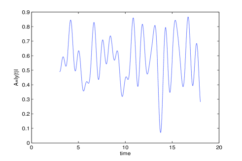
Figure 1: Amplitude A(t), defined by equation (22), of the signal $y(t)$ defined by equation (21).

For this signal, tPD considerably improves the result for $t\in\left[0,3\right]$ and $t\in\left[18,20\right]$, as it is easy to understand since the phase derivative of a random signal may have large local values but the corresponding amplitude of the total signal be small.

After using the tPD, we summarize the performances of the different tools in the following Table 1 in terms of their $sdev$.

sdev	$TDM$	$TDM+LM_{5}$	$TDM+TBD$	$TDM+TBD+LM_{5}$
$A(t)=1$	38.5 rd/s	4.5 rd/s	1.8 rd/s	1.5 rd/s
$A(t)\neq 1$	51 rd/s	11.2 rd/s	1.9 rd/s	1.5 rd/s
	$TNM$	$TNM+LM_{5}$	$TNM+TBD$	$TNM+TBD+LM_{5}$
$A(t)=1$	23.5 rd/s	3.9 rd/s	1.8 rd/s	1.5 rd/s
$A(t)\neq 1$	39.3 rd/s	10.7 rd/s	1.3 rd/s	2.2 rd/s

Table 1: Comparison of the different tools in terms of their $sdev$ for the signal $y_{0}$ defined by (21).

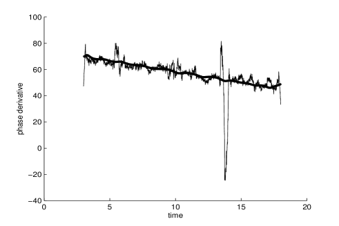
Figure 2: Phase derivative of $y_{0}(t)$, defined by equation(21) for the case $A(t)\neq 1$, using TDM+LM ($LM_{5}$) and TDM+TBD (bold line) on the tomogram for $\theta=\frac{\pi}{5}$.

In Fig.2 we show the graphic representation of the reconstructed phase derivative, for $A(t)\neq 1$, corresponding to TDM+LM ($LM_{5}$) and TDM+TBD of Table 1. As can be seen, the combined use of the tools described in section 2 allows a very efficient reconstruction of the phase derivative in this case, except when the signal is very small, for $t\approx 14s$. In particular TDM (or TNM )+ TBD gives very good results for an amplitude varying signal. It is however worthwhile to mention that the tomogram spectral family (8) is particularly well adapted to this type of ”incident wave” since in the limit case of an infinite time domain the corresponding spectrum would be reduced to a unique $c_{x}^{\theta}(f)$. But if, on one hand, we take advantage of this fact because the incident wave in reflectometry has this shape, on the other hand, the next example shows that the good performances of the tool are not limited to this particular non linear phase shape.

We also notice from Table 1 that, even before filtering, the normalisation TNM improves the results. This arises mostly from the processing of the small amplitudes regions.

Let now consider the ”deformed reflected chirp” $y_{R}(t)$ defined by :

$$y_{R}(t)=A(t)e^{i\Phi_{R}(t)}+b(t),t\in\left[0,20\right]s$$ (23)

where $\Phi_{R}(t)=a_{R}t^{2}+b_{R}t+10t^{\frac{3}{2}}$ and $a_{R}$, $b_{R}$ are chosen to have $\partial_{t}\phi(0)=75rd/s$ and $\partial_{t}\phi(20)$=50 rd/s. As before $A(t)$ is $one$ in the first case and defined by (22) in the second case with, in each case, a noisy component $b(t)$ with $SNR=10dB$.

The performances of the different tools, summarised in Table 2 in terms of their $sdev$, show how the tomogram based tools perform very accurate estimations of the (local) phase derivative in cases where other methods may have some difficulties. In particular, TBD seems a very efficient method to denoise the signal as it can be seen in the Fig.3.

sdev	$TDM$	$TDM+LM_{5}$	$TBD$	$TBD+LM_{5}$
$A(t)=1$	27.1 rd/s	6.6 rd/s	2.0 rd/s	1.5 rd/s
$A(t)\neq 1$	92 rd/s	24.7 rd/s	3.0 rd/s	2.9 rd/s
	$TNM$	$TNM+LM_{5}$	$TNM+TBD$	$TNM+TBD+LM_{5}$
$A(t)=1$	27.1 rd/s	4.7 rd/s	2.0 rd/s	1.5 rd/s
$A(t)\neq 1$	36.1 rd/s	14.1 rd/s	2.2 rd/s	1.4 rd/s

Table 2: Comparison of the different tools in terms of their $sdev$ for the signal $y_{R}$ defined by (23).

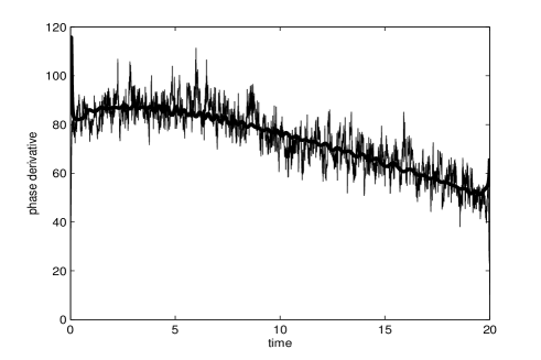
Figure 3: Phase derivative of $y_{R}(t)$, defined by equation(23) for the case $A(t)\neq 1$, using TDM+LM ($LM_{5}$) and TDM+TBD (bold line) on the tomogram for $\theta=\frac{\pi}{5}$.

4 Application to reflectometry data

We now show the ability of the tomographic methods to extract the phase derivative of an experimental signal coming from reflectometry measurements during a discharge in the Tore Supra at Cadarache.

The sweep-frequency reflectometry system of Tore Supra launches a probing wave on the extraordinary mode polarization (X mode) in the V band (50–75 GHz) [6], [7],  [13]. The emitting and receiving antennas are located at about 1.20 m from the plasma edge, outside the vacuum vessel. The reflectometry system repeatedly sends sweeps of duration $20\mu s$. The heterodyne reflectometers, with $I/Q$ detection, provide a good Signal to Noise Ratio, up to $40dB$. For each sweep, the reflected chirp $E_{R}(t)$ is mixed with the incident sweep $E_{0}(t)$ and only the interference term is recorded as an in-phase and a $90^{\circ}$ phase shifted sampled signals:

$$x_{1}(t)=A_{0}A_{R}(t)\cos(\varphi(t))$$

$$x_{2}(t)=A_{0}A_{R}(t)\sin(\varphi(t))$$

Let the reflected signal be

$$y(t)=x_{1}(t)+ix_{2}(t)=A(t)e^{i\varphi(t)}$$ (24)

The phase derivative of the signal corresponding to the plasma component of $y(t)$ is used to localize the cut-off density in the plasma. The amplitude of this signal $A(t)=A_{0}A_{R}(t)$ corresponds to a low frequency. The real part of the signal $y(t)$ is shown in Fig.4.

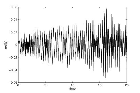
Figure 4: Time representation of the reflectometry signal (real part).

The tomogram at $\theta=\frac{3\pi}{10}$ was used to perform the factorization of the signal in [9]. Cutting the spectrum at $\epsilon=0.05$ max($\left|c_{x_{n}}^{\theta}(y)\right|$) the signal is factorized in three components as shown on Fig.5.

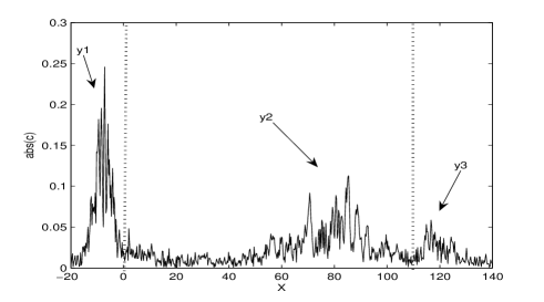
Figure 5: Spectrum $c^{\theta}_{x_{n}}(y)$ of the reflectometry signal $y(t)$ for $\theta_{0}=\frac{3\pi}{10}$ used in the factorization.

4.1 First component, the reflection on the porthole

The first component, $y_{1}(t)$, of the reflectometry signal is a low frequency signal corresponding to the heterodyne product of the probe signal with the reflection on the porthole [13]. This complex signal is written :

$$y_{1}(t)=A_{1}(t)e^{i\varphi_{1}(t)}$$ (25)

The phase derivative $\partial_{t}\varphi_{1}(t)$ may be positive and proportional to the time $\tau_{1}$ of the reflection of the probe signal on the porthole. If not, the reflectometry signal $y(t)$ defined by (24) is multiplied by $e^{iat}$ for some $a$ to calibrate the measurement. The real part and the modulus of $y_{1}(t)$ are shown in Fig.6.

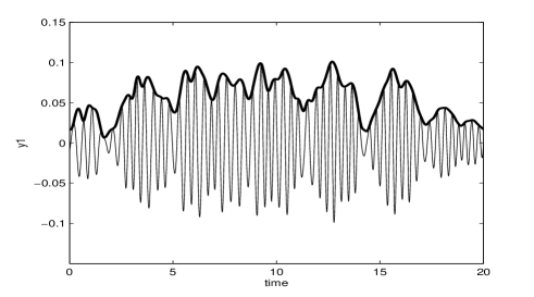
Figure 6: First component of the reflectometry signal corresponding to the reflection on the porthole (modulus and real part).

The phase derivative of $y_{1}(t)$ was then computed using TDM and shown in Fig.7. The mean value of the phase derivative is equal to $-16.4$ $rd/s$ and its sdev to $2.4rd/s$ (less than $15$ $\%$) in agreement with a rough estimation based on a spectrogram technique (see section 5). Since the phase derivative of $y_{1}(t)$ is negative, the reflectometry signal $y(t)$ had to be calibrated to set $\partial_{t}\varphi_{1}(t)$ proportional to $\tau_{1}$ (see conclusion).

We also shift the phase derivative of the other components by the same value.

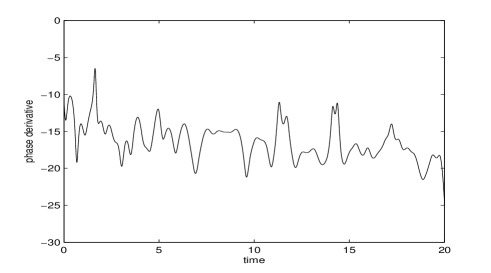
Figure 7: Phase derivative of the first component of the reflectometry signal corresponding to the reflection on the porthole, using TDM on the tomogram for $\theta=\frac{3\pi}{10}$.

4.2 Second component, the plasma signal

The second component has a Fourier spectra that fits the expected behavior corresponding to the reflection of the wave inside the plasma of the Tore Supra [13]. This component, $y_{2}(t)$ is defined as:

$$y_{2}(t)=A_{2}(t)e^{i\varphi_{2}(t)}$$ (26)

The modulus and real part are displayed together in the same plot (Fig.8).

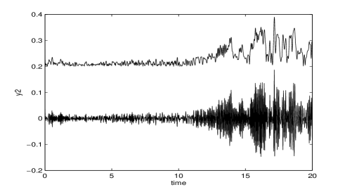
Figure 8: Modulus and real part of the second component of the reflectometry signal, corresponding to the reflection on the plasma. For visual puposes, the average of the modulus is shifted by 0.2.

Even if the modulus is of low frequency in comparison to the real part of $y_{2}(t)$, the modulus is not constant. In particular the signal is very small in the first half.

The amplitude of the signal $y_{2}$, for $t\in[0,11]s$, is very small in comparison to the amplitude for $t\in[11,20]s$. The power ratio of the signal $y_{2}$ for $t\in[0,11]s$ to the one for $t\in[11,20]s$ equals $0.035$ (SNR $\approx-15$ dB). Then the first part of the signal can be considered as filtered noise and , with tPD, the phase derivative will not be computed. This fact may correspond to the difficulty of the incident wave to reach the plasma in the first (lower) band of ”instantaneous frequencies” and therefore to a bad accuracy in the detection of the low densities present at the border of the plasma in tokamaks.

The phase derivative of the last part of the signal, for $t\in[11,20]s$, corresponding to TDM and TDM+LM are shown in Fig.9.

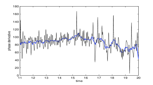
Figure 9: Phase derivative of the second component of the reflectometry signal for $t\in[11,20]s$. TDM and the TDM+LM filtered phase derivative ($LM_{15}$ : bold) are presented on the same plot.

For comparison, the $LM_{15}$ filtered phase derivative of the TDM and of the TNM (bold), for $t\in[11,20]s$, are plotted on the same Fig.10. The results are nearly the same, except for small differences for $t\approx 19.5s$ where the amplitude of the signal is very small.

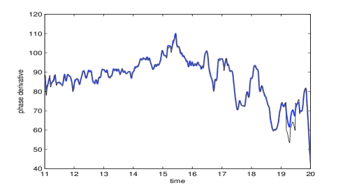
Figure 10: For $t\in[11,20]s$, $LM_{15}$ filtered phase derivative of the second component of the reflectometry signal obtained with TDM (thin line) and TNM (bold line).

We conclude that combining TDM (or TNM) with LM gives an accurate estimation of the phase derivative of the plasma component. TNM appears to be performant when the amplitude of the signal small. This claim will be confirmed by a comparison with the usual spectrogram analysis in section 5.

4.3 Third component, the multireflection

The last component of the reflectometry signal corresponds, [13] [9], to multireflections of the wave on the wall of the vacuum vessel. This component, $y_{3}(t)$ is written as :

$$y_{3}(t)=A_{3}(t)e^{i\varphi_{3}(t)}$$ (27)

The modulus $A_{3}(t)$ and the real part of $y_{3}(t)$ are presented together on the same figure (Fig.11). As compared to the real part of $y_{3}(t)$, the modulus $A_{3}(t)$ is a low frequency signal. We notice that for $t>13s$ the modulus is very small.

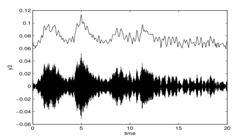
Figure 11: Modulus (bold) and real part of the third component of the reflectometry signal, corresponding to multi reflections on the vessel. For visual puposes, the average of the modulus is shifted by 0.06.

The phase derivative of $y_{3}(t)$ estimated using TDM+LM is plotted in Fig.12.

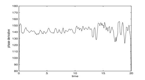
Figure 12: Phase derivative of the third component of the reflectometry signal, corresponding to multi reflections on the vessel, using TDM+LM ($LM_{15}$)on the tomogram for $\theta=\frac{3\pi}{10}$.

4.4 Components comparison

The LM filtered phase derivative of the three components of the reflectometry signal are plotted together on the same figure (Fig.13). It is instructive to compare these phase derivatives. For the first component, the phase derivative $\partial_{t}\varphi_{1}(t)$ is almost constant. This is because the phase $\varphi_{1}(t)$ is mainly due to a simple reflection on a nearby object, the porthole. The reflection on the plasma is quite complex. The first part of the signal should be considered as filtered noise and shows that there is a problem in reconstructing the density profile corresponding to this part of the sweep. The phase derivative of the third component of the signal, corresponding to multi reflections on the vessel, presents some similarities with the phase derivative of the first component, except for $t>14.5s$. It will eventually be interesting to factorize again this component if some information related to the properties of the plasma close to the vessel walls can be extracted from it. The modulus of the three components are low frequency signals, compared to the signals themselves. Usually, the phase derivative obtained by TDM is accurate when filtered by LM. In this case TBD does not seem adequate for denoising purposes, because it correlates with the component analysis and may eventually corrupt the factorization of the signal.

Figure 13: Phase derivative of the three components of the reflectometry signal, obtained with TDM+LM ($LM_{15}$). The mean value of $\partial_{t}\varphi_{1}(t)$ is equal to -18 $rd/s$, $\partial t\varphi_{2}(t)$ to 75 $rd/s$ and of $\partial t\varphi_{3}(t)$ to 140 $rd/s$.

5 Tomograms and spectrogram analysis

In this section we obtain the ”frequency” of the signal as a function of time, obtained by a moving window FFT spectrogram, and compare it with the phase derivative obtained by the tomographic techniques described before. The spectrogram is computed with a 64 points length window (the $grain$) and a $75\%$ overlap rate using the maximum pick method [12], allowing a FFT resolution of $10rd/s$ on $121$ time points. We avoided an estimation with higher time resolution because of FFT resolution constraints. For the tomographic phase derivative estimation we used, as usually, TDM (or TNM) together with LM filtering.

For the simulated ”deformed reflected chirp” $y_{R}(t)$ (Eq 23), figure 14 shows that a tomogram based technique gives a much better agreement with the known analytical phase derivative.

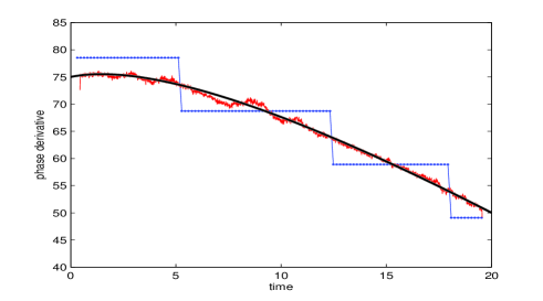
Figure 14: Phase derivative of $y_{R}(t)$ defined by (23) using TDM+TBD on the tomogram for $\theta=\frac{\pi}{5}$. The bold line is the analytical curve of the phase derivative. For comparison the dotted lines correspond to the maxima of a moving window FFT spectrogram with a resolution $\pm 9.9rd/s$ (see section 5).

For the three components of the plasma signal we have no way to directly verify the accuracy of the tomographic estimates, because the computed phase derivative is not exempt from noisy corruption. But in any case the corresponding spectrogram plots show (Figs.15, 16 and 17) that the tomogram allows for a good time resolution and in no case departs from the approximate values obtained in the corresponding spectrograms.

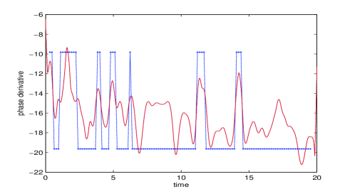
Figure 15: For the first component of the reflectometry signal, corresponding to the reflexion on the porthole phase derivative obtained by TDM+LM ($LM_{15}$). The dots are the maximum of a moving window FFT spectrogram with a resolution of $\pm 9.9rd/s$ .

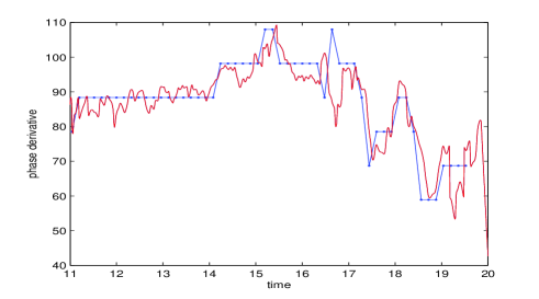
Figure 16: For last part ($t\in\left[11,20\right]s$) of the second component of the reflectometry signal, corresponding to the reflexion on the plasma : phase derivative obtained by TDM+LM ($LM_{15}$). The dots are the maximum of a moving window FFT spectrogram with a resolution of $\pm 9.9rd/s$ .

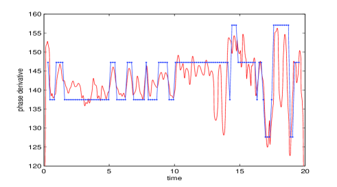
Figure 17: For the third component of the reflectometry signal, corresponding to multi reflexion phase derivative obtained by TDM+LM ($LM_{15}$). The dots are the maximum of a moving window FFT spectrogram with a resolution of $\pm 9.9rd/s$.

6 Remarks and conclusions

The tomographic technique for component analysis and computation of the phase derivative seems to provide an useful tool for the analysis of reflectometry signals. The component separation technique contains more information than the classical filtering techniques that have been used in the past. In addition, the TDM method of phase derivative calculation associated to LM filtering compares favorably with those obtained by spectrograms. Nevertheless, a few issues must be addressed:

1. How many components should be separated? [9]

From the tomogram itself one must decide how many components should be extracted from the signal. From the analysis of a great number of reflectometry signals it turned out that in some cases the third component, corresponding to the multireflections, was very weak. Maybe, in this case, only two components should be extracted.

2. Separation of the components: for which $\theta_{0}$ should the separation be performed?

For $\theta\approx 0$, the spectrum $\left\{c_{n}(\theta)\right\}$ is very close to the time representation of the signal. Then, the coefficients $c_{n}(\theta)$ are almost all different from $0$, and it is not possible to make the separation of the components. For $\theta\approx\frac{\pi}{2}$, the spectrum $\left\{c_{n}(\theta)\right\}$ is very close to the frequency representation of the signal. Then, many coefficients $c_{n}(\theta)$ are equal to $0$ and the separation can be performed. But it is not the best choice. The best choice for $\theta_{0}$ is where the spectrum still has many non null coefficients $c_{n}(\theta)$ and where it is still possible to make the separation by looking for concentrations of the tomographic probability. In the case of the reflectometry signals, the best choices seem to be around $\theta_{0}=\frac{3\pi}{10}$ (see Fig.5).

3. How is the phase derivative $\partial_{t}\phi(t)$ extracted?

3.1 First, one uses the time representation of the components to decide if all parts of the signal are relevant, or if some of it is just filtered noise (this is the case for the initial time interval in the second component of the reflectometry signals)

3.2 Then, extract the phase derivative using TDM on the tomogram for $\theta_{0}$ (For the first component of the reflectometry signal this was sufficient to extract the phase derivative which is almost constant).

3.3 The use of LM filtering on the phase derivative can be relevant. For the second and third component it seems necessary to apply a $LM_{15}$ low pass filter on the phase derivative.

4. The reflection on the porthole can be used to calibrate the measurements. This reflection can be detected after the time $\tau_{1}$ corresponding to the traveling wave from the emitting antenna to the receiver antenna. The group delay $\tau_{g1}$ of the first reflection, computed from the phase derivative should be equal to $\tau_{1}$.

The calibration of the measurements can be done by shifting the group delay $\tau_{g}$, obtained for each component from the phase derivative, by the quantity $\Delta\tau=\tau_{1}-\tau_{g1}$.

Acknowledgements: The work reported in this paper is an ongoing collaboration between the Center for Theoretical Physics (CNRS) - Marseille, the Department of Research on Controlled Fusion (CEA) - Cadarache and the Instituto de Plasmas e Fusão Nuclear (IST) - Portugal. We acknowledge financial support from Euratom/CEA (Contract No. V3517.001) and Euratom Mobility. We are also grateful to F. Clairet, from Cadarache, for given us access to the reflectometry data.

References

- [1] F. Simonet; Measurement of electron density profile by microwave reflectometry on tokamaks, Rev. Sci. Instrum. 56 (1985) 664-669.
- [2] P. Varela, M. E. Manso and A. Silva; Review of data processing techniques for density profile evaluation from broadband FM-CW reflectometry on ASDEX Upgrade, Nuclear Fusion 46 (2006) S693-S707.
- [3] P. Varela, M. E. Manso, I. Nunes, A. Silva and F. Silva; Automatic evaluation of plasma density profiles from microwave reflectometry on ASDEX upgrade based on the time-frequency distribution of the reflected signals, Rev. Sci. Instrum. 70 (1999) 1060-1063.
- [4] F. Nunes, M. E. Manso, I. Nunes, J. Santos, A. Silva and P. Varela; On the application of the Wigner-Ville distribution to broadband reflectometry, Fusion Engineering and Design 43 (1999) 441-449.
- [5] J. P. Bizarro and A. C. Figueiredo; The Wigner distribution as a tool for time-frequency analysis of fusion plasma signals: application to broadband reflectometry signals, Nuclear Fusion 39 (1999) 61-82.
- [6] F. Clairet, C. Bottereau, J. M. Chareau, M. Paume and R. Sabot; Edge density profile measurements by X-mode reflectometry on Tore Supra, Plasma Phys. Control. Fusion 43 (2001) 429-442.
- [7] F. Clairet, R. Sabot, C. Bottereau, J. M. Chareau, M. Paume, S. Heureaux, M. Colin, S. Hacquin and G. Leclert; X-mode heterodyne reflectometer for edge density profile measurements on Tore Supra, Rev. Sci. Instrum. 72 (2001) 340-343.
- [8] F. Silva, M. E. Manso, P. Varela and S. Hereaux; A 2d fdtd full-wave code for simulating the diagnostic of fusion plasmas with microwave reflectometry, Proc. Comp. Meth. in Eng. and Sci. (Macau, China) pp. 955-961.
- [9] F. Briolle, R. Lima, V. I. Man’ko and R. Vilela Mendes; A tomographic analysis of reflectometry data I: Component factorization, arXiv:0807.2744.
- [10] V. I. Man’ko and R. Vilela Mendes; Noncommutative time–frequency tomography, Phys. Lett. A 263 (1999) 53–59.
- [11] M. A. Man’ko, V. I. Man’ko and R. Vilela Mendes; Tomograms and other transforms: a unified view, J. Phys. A: Math. Gen. 34 (2001) 8321-8332.
- [12] B. Boashash; Estimating and interpreting the instantaneous frequency of a signal (parts 1 and 2), Proc. IEEE 80 (1992) 520-538 and 540-568.
- [13] F. Clairet, C. Bottereau, J. M. Chareau and R. Sabot; Advances of the density profile reflectometry on TORE SUPRA, Rev. Sci. Instrum. 74 (2003) 1481-1484.