Spacetime analogue of Bose-Einstein condensates: Bogoliubov-de Gennes formulation

Abstract

We construct quantum field theory in an analogue curved spacetime in Bose-Einstein condensates based on the Bogoliubov-de Gennes equations, by exactly relating quantum particles in curved spacetime with Bogoliubov quasiparticle excitations in Bose-Einstein condensates. Here, we derive a simple formula relating the two, which can be used to calculate the particle creation spectrum by solving the time-dependent Bogoliubov-de Gennes equations. Using our formulation, we numerically investigate particle creation in an analogue expanding Universe which can be expressed as Bogoliubov quasiparticles in an expanding Bose-Einstein condensate. We obtain its spectrum, which follows the thermal Maxwell-Boltzmann distribution, the temperature of which is experimentally attainable. Our derivation of the analogy is useful for general Bose-Einstein condensates and not limited to homogeneous ones, and our simulation is the first example of particle creations by solving the Bogoliubov-de Gennes equation in an inhomogeneous condensate.

I Introduction

Since the establishment of the theory of general relativity by A. Einstein, the study of classical gravity has been greatly extended. It provides some fascinating research subjects, especially cosmology and black holes. These two topics are powerful motivations for studying physics in curved spacetime.

The quantum effects of matter fields in curved spacetime is also important for studying cosmology and black hole physics. In standard modern cosmology, our Universe began with an accelerated expansion, known as inflation. The quantum effect of matter fields in the inflationary universe is believed to give rise to cosmological structures such as galaxies. However, this is merely theoretical scenario lacking any experimental evidence. Another example relates to the very mysterious objects known as black holes. According to S. W. Hawking’s prediction hawking , black holes are not completely black but rather they emit black body radiation through particle creation in the curved spacetime. It is very difficult to confirm this surprising phenomenon experimentally due to the extreme low intensity of the emitted radiation.

With such a background, new attempts to discover analogous phenomena in fluid systems have appeared. In a pioneering study, Unruh found that Hawking radiation is not restricted to gravity fields but that it can also be observed in a perfect fluid with a sonic horizon unruh81 . The basic concept involves identifying a sound wave propagating in a flowing fluid with a scalar field in curved spacetime. In this identification, fluid flow corresponds to curved spacetime and provides the spacetime metric. The sound wave can then be considered as a field in curved spacetime. This analogy has been applied not only to Hawking radiation but also to other field theoretical phenomena in curved spacetime, including cosmological particle creation novello2002 ; Barcelo:2005fc .

One of the merits of considering such an analogy lies in possibility of observing quantum effects in a laboratory. For the purpose of performing a precise investigation of quantum effects, we should consider quantum fluids. Bose-Einstein condensates (BECs) in trapped cold atoms represent one of the best systems in this context Anderson-95 ; Ketterle95 ; Pethick , for the following three reasons: (i) a BEC system is quite dilute and weakly interacting, so that its microscopic theory can be easily studied, (ii) many physical parameters of BECs are experimentally controllable, and (iii) various quantum phenomena of BECs can be directly observed, in stark contrast with other quantum fluids, such as superfluid helium systems. Therefore, BECs are one of the most promising quantum fluids for an analogous system.

In this spacetime analogy, spacetime corresponds to the condensate wave function described by the Gross-Pitaevskii (GP) equation GP ; Gross . Furthermore, quanta of the scalar field in spacetime correspond to Bogoliubov quasiparticles, which are low energy excitations on condensates and can be described by the Bogoliubov-de Gennes (BdG) equations. Bogoliubov quasiparticles not only exist in BECs at finite temperatures but they are also spontaneously created through the motion of BECs, which is one of the important problems associated with defining a BEC and its superfluidity in nonequilibrium Bose systems.

One of the main subjects of the analogy in BEC is to verify the Hawking radiation Garay-PRL ; Garay:2000jj ; Barcelo:2001ca ; Leonhardt02-1 ; Leonhardt02-2 ; Giovanazzi04 ; Giovanazzi:2004zv ; Wuester07 ; Kurita:2007bv ; Balbinot07 ; Carusotto08 ; Jain-PRA07 ; Wuester0805 . Not only the Hawking effect, other aspects of black hole physics as quasinormal frequencies or superradiance were also investigated Nakano:2004ha ; Basak:2005fv ; Federici:2005ty ; Barcelo:2006yi ; Takeuchi07 ; Barcelo:2007ru . Another stream is on cosmological models representing homogeneous expanding universe Barcero02 ; Barcero03 ; Lidsy03 ; Jain07 ; Weinfurtner:2008if ; Uhlmann0810 or inflationary universe Uhlmann0810 ; Fedichev03-1 ; Fedichev03-2 ; Fedichev03-3 ; Fischer04 ; Weinfurtner04 ; Uhlmann:2005hf . The analogy in BEC was firstly formulated by Garay et al. Garay-PRL and explored by Barceló et al. Barcelo:2000tg . In their formulation, the analogue geometry is read from a second-order differential equation for the perturbed phase of the condensate wave function which obeys the GP equation. In order to connect quantum physics in curved spacetime to the behavior of a realistic quantum fluid, Leonhardt et al. Leonhardt02-1 investigated the Hawking effect within the Bogoliubov theory of the elementary excitations in BEC. More detailed correspondence between the quanta in analogue spacetime and the Bogoliubov quasiparticles was discussed by Jain et al. Jain07 , giving an analytical expression for particle creation spectrum in terms of the Bogoliubov mode functions in the case of homogeneous BEC.

In this paper, we formulate the spacetime analogy in terms of the BdG equations as an extension of Leonhardt02-1 , by exactly relating Bogoliubov quasiparticles with quantum particles in curved spacetime. It is shown that the number operator of quanta in analogue spacetime is different from that of Bogoliubov quasiparticles, unless the corresponding field is normalized correctly. With the correct normalization, the number of quanta in analogue spacetime can be exactly related with that of Bogoliubov quasiparticles. Furthermore, it is shown that the orthonormal relation between the normalized mode functions exactly corresponds to that of BdG wave functions. We also explicitly define Bogoliubov quasiparticle creation as a phenomenon caused by a change in the complete set of BdG wave functions for the motion of a BEC, and we define analogue particle creation in terms of Bogoliubov quasiparticle creation. Our formulation based on the BdG equations is generally applicable and gives a simple formula for particle creation spectrum in terms of the Bogoliubov mode functions. In the derivation of the formula, we consider the correctly normalized field so that the formula is relevant quantitatively. Our derivation of the formula is different from that given in Jain07 , and consequently the formula is generalized to be applicable in general cases. Furthermore, our formulation is independent of whether condensates are homogeneous or inhomogeneous, and the obtained formula is valid even for inhomogeneous condensates.

We then perform a numerical simulation for the simplest quantum effect in analogue curved spacetime: particle creation by the analogue expanding Universe as an expanding BEC. The spectrum obtained is consistent with the thermal Maxwell-Boltzmann distribution, the temperature of which has already been achieved in actual experiments. In this simulation, we set the initial state for the excitation field to be vacuum just after the condensate starts to expand, and there is no external manipulation after the initial time and the particle creation occurs spontaneously, which should be contrasted to the previous works Barcero02 ; Barcero03 ; Lidsy03 ; Jain07 ; Weinfurtner:2008if . In this sense, the system is isolated. The particle creation simulated here is not a result of any perturbation but a field theoretical phenomenon caused by a difference in definition of quasiparticles.

This paper is organized as follows. In section II, we derive an analogue spacetime metric from the BdG equations. In section III, we construct quantum field theory on the analogue spacetime based on BdG theory. In section IV, we define Bogoliubov quasiparticle creation and give a formula for analogue particle creation. In section V, we show the results of a numerical simulation giving particle creation in an expanding and shrinking BEC in a trapping potential. The conclusions are given in section VI.

II Analogue spacetime in BEC

We start with the Hamiltonian describing bosons trapped by an external confining potential $V_{\mathrm{ext}}({\bf x})$ given by

$$H=\int d^{3}x\>\psi^{\dagger}({\bf x})\bigg{[} K+V_{\mathrm{ext}}({\bf x})-\mu$$

$$+\frac{1}{2}U_{0}\psi^{\dagger}({\bf x})\psi({\bf x})\bigg{]}\psi({\bf x}).$$ (1)

Here $\psi^{\dagger}({\bf x})$ and $\psi({\bf x})$ are boson field operators in the second quantized form, $K=-\hbar^{2}\nabla^{2}/2m$ is the kinetic energy operator, $U_{0}$ is the particle interaction strength and $\mu$ is the chemical potential FW71 ; Fetter1972 . In the Heisenberg picture, the field equation is given by

$$i\hbar\partial_{t}\psi({\bf x},t) =[K+V_{\mathrm{ext}}({\bf x})-\mu$$

$$\quad+U_{0}\psi^{\dagger}({\bf x},t)\psi({\bf x},t)]\psi({\bf x},t).$$ (2)

The density operator and the current density operator are respectively defined by

$$\hat{n}({\bf x},t) =\psi^{\dagger}({\bf x},t)\psi({\bf x},t),$$ (3)

$$\hat{\bf j}({\bf x},t) =\frac{\hbar}{2mi}[\psi^{\dagger}({\bf x},t)\nabla\psi({\bf x},t)$$

$$\qquad\qquad-\{\nabla\psi^{\dagger}({\bf x},t)\}\psi({\bf x},t)].$$ (4)

In a BEC, the field $\psi$ consists of two components, $\psi({\bf x},t)=\Psi({\bf x},t)+\phi({\bf x},t)$, where $\Psi({\bf x},t)\equiv\langle\psi({\bf x},t)\rangle$ describes the condensate PPO with $\langle O\rangle$ denoting a grand canonical ensemble average of $O$. The Bogoliubov field $\phi({\bf x},t)$ describes fluctuations about the condensate. The condensate wave function $\Psi({\bf x},t)$ obeys the following GP equation GP ; Gross ,

$$i\hbar\partial_{t}\Psi({\bf x},t) =\left[K+V_{\mathrm{ext}}({\bf x})-\mu\right]\Psi({\bf x},t)$$

$$\quad+U_{0}|\Psi({\bf x},t)|^{2}\Psi({\bf x},t).$$ (5)

The condensate wave function $\Psi({\bf x},t)$ is rewritten in terms of the amplitude, $|\Psi({\bf x},t)|=\sqrt{n_{0}({\bf x},t)}$, and the phase, $S({\bf x},t)$, as follows,

$$\Psi({\bf x},t)=\sqrt{n_{0}({\bf x},t)}e^{iS({\bf x},t)}.$$ (6)

Hereafter, the spatial and time dependence of fields, represented by $({\bf x},t)$, is implicit for conciseness of notation. The condensate contributions to the density and current density are

$$n_{0}=|\Psi|^{2},\quad{\bf j}_{0}=n_{0}\frac{\hbar}{m}\nabla S=n_{0}{\bf v}_{0},$$ (7)

where ${\bf v}_{0}:=\hbar\nabla S/m$ is the velocity of the condensate. With these quantities, the GP equation can be rewritten as two real equations

$$\hbar\partial_{t}S+n_{0}^{-1/2}K n_{0}^{1/2}+V_{\mathrm{ext}}-\mu+U_{0}n_{0}+\frac{m}{2}v_{0}^{2}=0,$$ (8)

$$\partial_{t}n_{0}+\nabla\cdot(n_{0}{\bf v}_{0})=0.$$ (9)

The first equation is Bernoulli’s equation for the condensate current and the second equation represents conservation of the current.

Density fluctuations and current density fluctuations are described by

$$\hat{\rho}^{\prime} =\Psi^{\ast}\phi+\phi^{\dagger}\Psi=\sqrt{n_{0}}(e^{-iS}\phi+e^{iS}\phi^{\dagger}),$$ (10)

$$\hat{\bf j}^{\prime} =\frac{\hbar}{2mi}[\Psi^{\ast}\nabla\phi+\phi^{\dagger}\nabla\Psi-(\nabla\Psi^{\ast})\phi-(\nabla\phi^{\dagger})\Psi].$$ (11)

Here, we take the linearized approximation, that is, we neglect higher order fluctuations, like $\phi^{\dagger}\phi$. The fluctuation fields $\phi,\phi^{\dagger}$ obey the BdG equations. These fields can be U(1) gauge transformed as

$$\tilde{\phi}:=e^{-iS}\phi,\quad\tilde{\phi}^{\dagger}:=e^{iS}\phi^{\dagger}.$$ (12)

The field equations are

$$i\hbar\partial_{t}\tilde{\phi} =(\tilde{L}+2U_{0}n_{0}+\hbar\partial_{t}S)\tilde{\phi}+U_{0}n_{0}\tilde{\phi}^{\dagger},$$ (13)

$$-i\hbar\partial_{t}\tilde{\phi}^{\dagger} =(\tilde{L}^{\ast}+2U_{0}n_{0}+\hbar\partial_{t}S)\tilde{\phi}^{\dagger}+U_{0}n_{0}\tilde{\phi},$$ (14)

where $\tilde{L}$ is defined as

$$\tilde{L} :=\tilde{K}+V_{ext}-\mu,\quad\tilde{K}:=e^{-iS}Ke^{iS}.$$ (15)

Performing a short calculation, one obtains

$$\tilde{K}=K-i\hbar{\bf v}_{0}\cdot\nabla-\frac{1}{2}i\hbar(\nabla\cdot{\bf v}_{0})+\frac{1}{2}mv_{0}^{2}.$$ (16)

With these fields, $\hat{\rho}^{\prime}$ and $\hat{\bf j}^{\prime}$ take the simple forms

$$\hat{\rho}^{\prime}=\sqrt{n_{0}}(\tilde{\phi}+\tilde{\phi}^{\dagger}),\quad\hat{\bf j}^{\prime}=\hat{\rho}^{\prime}{\bf v}_{0}+n_{0}\hat{\bf v}^{\prime},$$ (17)

where we have introduced $\hat{\bf v}^{\prime}=\nabla\hat{\Phi}^{\prime}$ with

$$\hat{\Phi}^{\prime}:=\frac{\hbar}{2mi\sqrt{n_{0}}}(\tilde{\phi}-\tilde{\phi}^{\dagger}).$$ (18)

Note that the field $\hat{\Phi}^{\prime}$ is the velocity potential in the first order approximation with respect to fluctuation fields.

Taking the difference of eqs. (13) and (14), we see that the operators $\hat{\rho}^{\prime}$ and $\hat{\bf j}^{\prime}$ obey the conservation law

$$\partial_{t}\hat{\rho}^{\prime}+\nabla\cdot\hat{\bf j}^{\prime}=0.$$ (19)

Therefore, the continuity equation is satisfied within first order terms for fluctuation fields. Under the hydrodynamic approximation, in which the density gradient is smooth over the local healing length $\xi=\hbar/\sqrt{2mU_{0}n_{0}}$, the sum of eqs. (13) and (14) yields

$$\hat{\rho}^{\prime}\simeq-\frac{m}{U_{0}}(\partial_{t}+{\bf v}_{0}\cdot\nabla)\hat{\Phi}^{\prime}.$$ (20)

Then, eq. (19) can be rewritten as

$$\left(\partial_{t}+\nabla\cdot{\bf v}_{0}\right)\frac{m}{U_{0}}(\partial_{t}+{\bf v_{0}}\cdot\nabla)\hat{\Phi}^{\prime}-\nabla\cdot\left(\frac{m}{U_{0}}c_{s}^{2}\nabla\hat{\Phi}^{\prime}\right)\simeq 0,$$ (21)

where $c_{s}:=\sqrt{U_{0}n_{0}/m}$. Now, we introduce a symmetric tensor

$$g_{\mu\nu}=\frac{\Lambda mc_{s}}{U_{0}}\left(\begin{array}[]{cc}-(c_{s}^{2}-v_{0}^{2})&-v_{0a}\\ -v_{0b}&\delta_{ab}\end{array}\right),$$ (24)

where $\Lambda$ is a constant and $a,b=1,2,3$. We can then write eq. (21) as

$$\frac{1}{\sqrt{-{\rm det}g}}\partial_{\mu}\left[\sqrt{-{\rm det}g}g^{\mu\nu}\partial_{\nu}\hat{\Phi}^{\prime}\right]=0.$$ (25)

If we identify $g_{\mu\nu}$ with a spacetime metric through $ds^{2}=g_{\mu\nu}dx^{\mu}dx^{\nu}$, the field $\hat{\Phi}^{\prime}$ obeys the equation of motion for a minimally coupled scalar field in curved spacetime with the metric (24), and can be seen to be a field in curved spacetime.

The equation for the field $\hat{\Phi}^{\prime}$ given in (21) was already derived as a perturbation equation of the GP equation, see for example Jain07 ; Weinfurtner:2007dq . In this section, we have rederived it directly from time dependent BdG equations as an extension of analysis given in Leonhardt02-1 . This derivation is physically equivalent to the original derivation of analogue metric given in Garay-PRL .

III Construction of quantum field theory in curved spacetime

Now, the field $\hat{\Phi}^{\prime}$ is found to be a corresponding field in analogue spacetime. In this section, however, we show that the number of quanta described by $\hat{\Phi}^{\prime}$ in the analogue spacetime does not quantitatively correspond to that of quasiparticles in BEC, and there is an exact expression for a quantum field in analogue spacetime which is different from $\hat{\Phi}^{\prime}$. To address this point, we construct quantum field theory on the analogue spacetime by using the BdG theory.

For that purpose, we introduce linear transformation and separate operators and wave functions so that the operators $\alpha_{j}$ and $\alpha_{j}^{\dagger}$ respectively become annihilation and creation operators, as

$$\tilde{\phi}=\sum_{j}[u_{j}\alpha_{j}-v_{j}^{\ast}\alpha^{\dagger}_{j}],\quad\tilde{\phi}^{\dagger}=\sum_{j}[u_{j}^{\ast}\alpha_{j}^{\dagger}-v_{j}\alpha_{j}].$$ (26)

The operators $\alpha_{j}$ and $\alpha_{j}^{\dagger}$ are set to satisfy the boson commutation relation $[\alpha_{j},\alpha_{k}^{\dagger}]=\delta_{jk}$. The wave functions $u_{j}$ and $v_{j}$ obey the following matrix equations:

$$i\hbar\partial_{t}\left(\begin{array}[]{c}u_{j}\\ v_{j}\end{array}\right)=\left(\begin{array}[]{cc}\tilde{W}&-U_{0}n_{0}\\ U_{0}n_{0}&-\tilde{W}^{\ast}\end{array}\right)\left(\begin{array}[]{c}u_{j}\\ v_{j}\end{array}\right),$$ (33)

where $\tilde{W}:=\tilde{L}+2U_{0}n_{0}+\hbar\partial_{t}S$. They then satisfy the orthonormal conditions

$$\begin{array}[]{c}\displaystyle\int d^{3}x\>(u_{j}^{\ast}u_{k}-v_{j}^{\ast}v_{k})=\delta_{jk},\\ \displaystyle\int d^{3}x\>(u_{j}u_{k}-v_{j}v_{k})=0.\end{array}$$ (36)

The operators $\alpha_{j}$ and $\alpha_{j}^{\dagger}$ describe the annihilation and creation of Bogoliubov quasiparticles, respectively. Here, we identify these with annihilation and creation operators of quanta in the analogue spacetime.

The field $\hat{\Phi}^{\prime}$ is expanded in terms of operators by use of the expansion (26).

$$\hat{\Phi}^{\prime}=\sum_{j}\left[\alpha_{j}\tilde{f}_{j}+\alpha^{\dagger}_{j}\tilde{f}^{\ast}_{j}\right],$$ (37)

where $\tilde{f}_{j}$ is defined as

$$\tilde{f}_{j}:=\frac{\hbar}{2mi\sqrt{n_{0}}}(u_{j}+v_{j}).$$ (38)

Firstly, we check that the coefficient functions $\tilde{f}_{j}$ satisfies the relativistic wave equation with the metric (24). Eq. (8) leads to

$$\tilde{W}=K^{\prime}+U_{0}n_{0}-i\hbar D_{v},$$ (39)

with these definitions $K^{\prime}:=K-n_{0}^{-1/2}(Kn_{0}^{1/2})$ and

$$D_{v}:={\bf v}_{0}\cdot\nabla+\frac{1}{2}(\nabla\cdot{\bf v}_{0}).$$ (40)

The matrix equation (33) then gives equations for the functions $u_{j}+v_{j}$ and $u_{j}-v_{j}$ as

$$i\hbar\left(\partial_{t}+D_{v}\right)(u_{j}+v_{j}) \approx 2U_{0}n_{0}(u_{j}-v_{j}),$$ (41)

$$i\hbar\left(\partial_{t}+D_{v}\right)(u_{j}-v_{j}) =K^{\prime}(u_{j}+v_{j}),$$ (42)

where the hydrodynamic approximation,

$$K^{\prime}+2U_{0}n_{0}\approx 2U_{0}n_{0},$$ (43)

has been used. From eq.(41),

$$u_{j}-v_{j}=\frac{i\hbar}{2U_{0}n_{0}}\left(\partial_{t}+D_{v}\right)(u_{j}+v_{j}).$$ (44)

Substituting this into eq.(42), we obtain

$$(\partial_{t}+D_{v})\frac{1}{U_{0}n_{0}}(\partial_{t}+D_{v})(u_{j}+v_{j})+\frac{2}{\hbar^{2}}K^{\prime}(u_{j}+v_{j})=0.$$ (45)

The conservation of the condensate current (9) leads to

$$\left(\partial_{t}+{\bf v}_{0}\cdot\nabla\right)\frac{X}{\sqrt{n_{0}}}=\frac{1}{\sqrt{n_{0}}}\left(\partial_{t}+D_{v}\right)X,$$ (46)

$$(\partial_{t}+D_{v})\frac{1}{\sqrt{n_{0}}}X=\frac{1}{\sqrt{n_{0}}}\left(\partial_{t}+\nabla\cdot{\bf v}_{0}\right)X,$$ (47)

for any function $X$. Therefore, we obtain

$$\left(\partial_{t}+\nabla\cdot{\bf v}_{0}\right)\frac{1}{U_{0}}(\partial_{t}+{\bf v}_{0}\cdot\nabla)\tilde{f}_{j}$$

$$+\frac{2}{\hbar^{2}}\sqrt{n_{0}}K^{\prime}\sqrt{n_{0}}\tilde{f}_{j}=0.$$ (48)

Furthermore, by noting that

$$K^{\prime}\sqrt{n_{0}}X=-\frac{\hbar^{2}}{2m}\frac{1}{\sqrt{n_{0}}}\nabla\cdot(n_{0}\nabla X),$$ (49)

one finds that the functions $\{\tilde{f}_{j}\}$ satisfy

$$\partial_{\mu}\left[\sqrt{-{\rm det}g}g^{\mu\nu}\partial_{\nu}\tilde{f}_{j}\right]=0,$$ (50)

with metric (24), as expected.

Now, we calculate the Klein-Gordon (KG) inner product between functions $\{\tilde{f}_{j}\}$ in the analogue spacetime, which is a conserved product for solutions to the wave equation in curved spacetime. The KG product for functions $F$ and $G$ is defined as

$$(F,G)_{KG}=-i\int_{\Sigma}(Fn^{\mu}\partial_{\mu}G^{\ast}-G^{\ast}n^{\mu}\partial_{\mu}F)\sqrt{{\rm det}h}\>d^{3}x,$$ (51)

where $n=n^{\mu}\partial_{\mu}$ is a unit normal vector orthogonal to the spacelike surface $\Sigma$, that is, $n$ is a future-directed timelike vector. $\sqrt{{\rm det}h}\>d^{3}x$ is an invariant volume element of the surface $\Sigma$. $h_{ab}$ is the induced metric on $\Sigma$. If $F$ and $G$ are solutions of the Klein-Gordon equation (50), the value $(F,G)_{KG}$ does not depend on the choice of $\Sigma$ as long as $\Sigma$ is a Cauchy surface BD . If we choose a $t$-constant surface as $\Sigma$, the induced metric is

$$ds^{2}_{\Sigma}=h_{ab}dx^{a}dx^{b}=\frac{m\Lambda}{U_{0}}c_{s}\delta_{ab}dx^{a}dx^{b}.$$ (52)

Then, we obtain $\sqrt{{\rm det}h}=(m\Lambda c_{s})^{3/2}U_{0}^{-3/2}$. The normal vector to the surface is

$$n^{\mu}\partial_{\mu}=c_{s}^{-3/2}\sqrt{\frac{U_{0}}{m\Lambda}}(\partial_{t}+{\bf v}_{0}\cdot\nabla).$$ (53)

By using eqs. (46) and (41), the KG product between the coefficient functions can be calculated as

$$(\tilde{f}_{j},\tilde{f}_{k})_{KG}=\frac{\Lambda\hbar}{m}\int_{\Sigma}d^{3}x\>\left[u_{j}u_{k}^{\ast}-v_{j}v_{k}^{\ast}\right].$$ (54)

Using the orthonormal relation (36), we obtain

$$(\tilde{f}_{j},\tilde{f}_{k})_{KG}=\frac{\Lambda\hbar}{m}\delta_{jk}.$$ (55)

Similar calculations show that $(\tilde{f}_{j}^{\ast},\tilde{f}_{k}^{\ast})_{KG}=-\frac{\Lambda\hbar}{m}\delta_{jk}$ and $(\tilde{f}_{j},\tilde{f}_{k}^{\ast})_{KG}=0$. Therefore, it is seen that the coefficient functions are normal each other. At the same time, it is also seen that they are not orthonormal. We find that a set of functions

$$\frac{\sqrt{m}}{\sqrt{\Lambda\hbar}}\tilde{f}_{j},$$ (56)

is a set of orthonormal mode functions for the field $\hat{\Phi}^{\prime}$. Then the number operator of quanta described by $\hat{\Phi}^{\prime}$ is

$$\tilde{N}_{j}=\frac{\Lambda\hbar}{m}\alpha_{j}^{\dagger}\alpha_{j}.$$ (57)

The number of quanta in analogue spacetime does not correspond to that of Bogoliubov quasiparticles. In order to identify these numbers, the field has to be normalized so as to make the coefficient functions orthonormal. It is easily seen that a set of functions

$$f_{j}:=\frac{\sqrt{\hbar}}{2i\sqrt{\Lambda mn_{0}}}(u_{j}+v_{j}),$$ (58)

is a complete set in quantum field theory in analogue curved spacetime, that is, these functions satisfy

$$(f_{j},f_{k})_{KG}=\delta_{jk}.$$ (59)

Then the normalized field is

$$\varphi=\sum_{j}\left[\alpha_{j}f_{j}+\alpha^{\dagger}_{j}f^{\ast}_{j}\right]=\frac{\sqrt{m}}{\sqrt{\Lambda\hbar}}\hat{\Phi}^{\prime}.$$ (60)

Then, the number operator of the field $\varphi$ is

$$N_{j}=\alpha_{j}^{\dagger}\alpha_{j}.$$ (61)

We have obtained orthonormal mode functions (58) and normalized scalar field (60) in the analogue spacetime from BdG wave functions. Equivalently, we have exactly related one Bogoliubov quasiparticle with one quantum in the analogue spacetime. Now, with this normalized field $\varphi$, quantum field theory in curved spacetime can be applicable to Bogoliubov quasiparticles quantitatively.

IV Particle creation

In this section, we discuss a simple example of particle creation and derive a formula connecting particle creation spectrum and BdG wave functions.

Let us consider a condensate which is static and having no excitation at initial time $t=t_{1}$. For $t_{1}<t<t_{2}$, the condensate evolves dynamically and, at $t=t_{2}$, it becomes static again. Then, the corresponding effective spacetime evolves dynamically and, in general, quantum field theory in curved spacetime will predict particle creation. Therefore, the analogy implies that, Bogoliubov quasiparticles will be created at $t=t_{2}$.

We choose a complete set at time $t=t_{\mathrm{\lambda}}$ ($\lambda=1,2$), $\{f_{j}^{(\lambda)}\}$, as each $f_{j}^{(\lambda)}$ consists of energy eigenfunctions of the BdG equations $u_{j}^{(\lambda)}$ and $v_{j}^{(\lambda)}$ at each time $t=t_{\mathrm{\lambda}}$. In this way, we define one particle state of the quantum by using annihilation and creation operators $\alpha_{j}^{(\lambda)}$ and $\alpha_{j}^{(\lambda)\dagger}$ which diagonalize the BdG Hamiltonian.

At the initial and final times $t=t_{\mathrm{\lambda}}$ ($\lambda=1,2$), we expand the field using a complete set at each time as

$$\varphi=\sum_{j}\left[\alpha_{j}^{(\lambda)}f^{(\lambda)}_{j}+\alpha^{(\lambda)\dagger}_{j}f^{(\lambda)\ast}_{j}\right],$$ (62)

These two sets are related to each other by linear transformations

$$f^{(2)}_{k}=\sum_{j}\left[A_{kj}f^{(1)}_{j}+B_{kj}f^{(1)\ast}_{j}\right].$$ (63)

Therefore, the creation and annihilation operators are related as

$$\alpha_{k}^{(2)}=\sum_{j}\left(A_{kj}^{\ast}\alpha_{j}^{(1)}-B_{kj}^{\ast}\alpha_{j}^{(1)\dagger}\right).$$ (64)

Since the initial condensate has no excitations, the state for $\varphi$ is in the initial vacuum denoted by $|0\rangle_{(1)}$, i.e., $\alpha_{j}^{(1)}|0\rangle_{(1)}=0$. We consider the Heisenberg picture and the state for $\varphi$ is not time-dependent. Then, the expectation value of the final number operator in the $j$-th mode $\hat{N}_{j}^{(2)}:=\alpha_{j}^{(2)\dagger}\alpha_{j}^{(2)}$ is calculated as

$${}_{(1)}\langle 0|\hat{N}_{j}^{(2)}|0\rangle_{(1)}=\sum_{k}|B_{jk}|^{2}.$$ (65)

If $B_{kj}$ is not zero for any $k$, then particles will be created. The expected total number of particles is thus tr($B^{\ast}B$).

We should note that solutions to the BdG equations $u_{j}$, $v_{j}$ solve relativistic wave equations (50) through the relation (58). Therefore, if the time-dependent BdG equations are solved, then the functions $\{f_{j}^{(1)}\}$ satisfy the equation of motion in time-dependent effective spacetime. Therefore, time evolution of the initial complete set in analogue spacetime is solved automatically. Then, the coefficient $B_{jk}$ is calculated as the KG product at the final time $t=t_{2}$,

$$B_{jk} =-(f_{j}^{(2)},f_{k}^{(1)\ast})_{KG}$$

$$=\int_{t=t_{2}}d^{3}x(u_{j}^{(2)}v_{k}^{(1)}-v_{j}^{(2)}u_{k}^{(1)}).$$ (66)

In the derivation of this formula, we have used (46) and (41) as in the calculation of (59). Here, it should be noted that, in the calculation of $B_{jk}$, not the set of functions $\{\tilde{f}_{j}\}$ but $\{f_{j}\}$ has to be considered so that the Bogoliubov coefficient $B_{jk}$ is relevant as a particle creation spectrum quantitatively. This expression for the Bogoliubov coefficient (66) was obtained in Jain07 for particle creation in homogeneous BEC. Now, the formula (66) has been shown to be valid for particle creation in dynamical condensates even when it is inhomogeneous, because, in our formulation, any simplification for the Bogoliubov mode functions is not needed to be assumed. Therefore, our formulation is much more powerful. It is powerful enough to show that the formula (66) is valid for general cases. In this way, the spectrum of particle creation (65) can be expressed in terms of the BdG wave functions via the formula (66).

Finally, we comment that the total number of particles

$$N=\int d^{3}x\>\langle\psi^{\dagger}\psi\rangle=\int d^{3}x\>(|\Psi|^{2}+\langle\phi^{\dagger}\phi\rangle),$$ (67)

is not conserved. $\partial_{t}N\neq 0$ in our model, since the conservation is closed only in the GP equation for the condensate particles;

$$\partial_{t}\int d^{3}x\>|\Psi|^{2}=0.$$ (68)

To overcome this unphysical result, we have to account for the quantum backreaction which is the effect of the dynamical development of the Bogoliubov field to the BEC. In this paper, we assume that the quantum backreaction can be neglected when the number of the BEC particles far exceeds the number of Bogoliubov quasiparticles.

V Numerical simulation

Now, we show a numerical simulation giving particle creation in an expanding and shrinking BEC in the trapping potential $V_{\mathrm{ext}}({\bf x})=m(\omega_{x}^{2}x^{2}+\omega_{y}^{2}y^{2}+\omega_{z}^{2}z^{2})/2$, where $\omega_{x}$, $\omega_{y}$, and $\omega_{z}$ are the trapping frequencies of the potential along the $x$, $y$, and $z$-axes respectively. We consider the case in which a BEC is tightly trapped only in the $x$-axis; $\omega_{x}\gg\omega_{y},\omega_{z}$, and apply the one-dimensional simulation by neglecting the spatial derivatives of the $y$ and $z$-axes. We find the stationary solution of the GP equation at the trapping frequency $\omega_{x}=\omega_{\mathrm{i}}$, and then change the frequency to $\omega_{x}=\omega_{\mathrm{f}}$ at $t=t_{1}=0$ to make the expanding and shrinking BEC. This situation can be interpreted as a cosmological expansion and contraction, because, in the expansion of condensate for example, the sound velocity becomes small and the time interval $\Delta t$ during which a particle on the condensate can travel over it,

$$\Delta t:=2\int^{R_{TF}}_{0}c_{s}^{-1}dx,$$ (69)

becomes long, where $R_{TF}$ is the Thomas-Fermi edge of the condensate. This implies that the size of the analogue spacetime measured by the sound velocity also expands. Furthermore, the sound velocity is not constant with respect to the spatial coordinate, which implies that the analogue spacetime is inhomogeneous. Therefore, the analogue spacetime corresponds to an inhomogeneous expanding universe. Similarly, a shrinking BEC corresponds to an inhomogeneous contracting universe.

Although the condensate starts to move due to changing the trapping frequency, we are not interested in particle creation caused by such an external manipulation but in spontaneous one as a quantum field theoretical phenomenon. For that purpose, we set vacuum for Bogoliubov quasiparticles at time just after changing the frequency, say $t=t_{1}+0$. This is the initial condition in this simulation. After $t=t_{1}+0$, therefore, the system is isolated without external manipulation, and particle creation can be regarded as a consequence of time evolving analogue spacetime.

The spectrum of particle creation $\sum_{k}|B_{jk}|^{2}$ can be calculated as follows. Firstly, we calculate the time evolution of $u_{j}^{(1)}$ and $v_{j}^{(1)}$ with that of the condensate wave function $\Psi$ by using eq. (33), starting from the quasi-steady solution at $t=t_{1}+0$:

$$E_{j}^{(\lambda)}\left(\begin{array}[]{c}u_{j}^{(\lambda)}\\ v_{j}^{(\lambda)}\end{array}\right)=\left(\begin{array}[]{cc}\tilde{W}&-U_{0}n_{0}\\ U_{0}n_{0}&-\tilde{W}^{\ast}\end{array}\right)\left(\begin{array}[]{c}u_{j}^{(\lambda)}\\ v_{j}^{(\lambda)}\end{array}\right).$$ (76)

Then, at $t=t_{2}$, we obtain $u_{j}^{(1)}$ and $v_{j}^{(1)}$ after the time evolution and $u_{j}^{(2)}$ and $v_{j}^{(2)}$ by using eq. (76) again. Finally, we obtain the spectrum of particle creation from eq. (66).

As the physical parameters, we use $m=1.44\times 10^{-25}$ kg, $\omega_{\mathrm{i}}=150\times 2\pi$ Hz, $\omega_{\mathrm{f}}=\omega_{\mathrm{i}}/\sqrt{2}$, and $\omega_{y}=\omega_{z}=\omega_{\perp}=50\times 2\pi$ Hz considering a BEC experiment of ⁸⁷Rb atoms, the total number of which is set to be $N=2.5\times 10^{6}$. As the coupling constant of atomic interactions $U_{0}$, we use $s$-wave scattering:

$$U_{0}=4\left[\frac{\hbar^{3}a^{3/2}\omega_{\perp}^{3}N^{3/2}}{15m^{1/2}\omega_{x}}\right]^{2/5},$$ (77)

with a scattering length of $a=5.61$ nm. As a numerical method, we use the fully dealiased Chebyshev-Galerkin method in space $-16a_{x}\leq x\leq 16a_{x}$ with the Dirichlet boundary condition and the Runge-Kutta-Gill method in time with $\Delta t=1\times 10^{-4}/\omega_{\mathrm{i}}$, where $a_{x}=\sqrt{\hbar/m\omega_{\mathrm{i}}}$ is the characteristic length defined by the trapping potential.

Figure 1(a) shows the time development of the Thomas-Fermi edge $R_{\mathrm{TF}}$ of the condensate fitted by a harmonic function. Dynamics of the condensate is almost periodic, and its period is $T\simeq 5.10/\omega_{\mathrm{i}}$ which is consistent with that of the breathing mode $\sim 2\pi/(\sqrt{3/2}\omega_{\mathrm{i}})$.

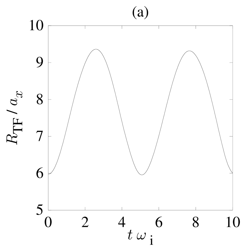
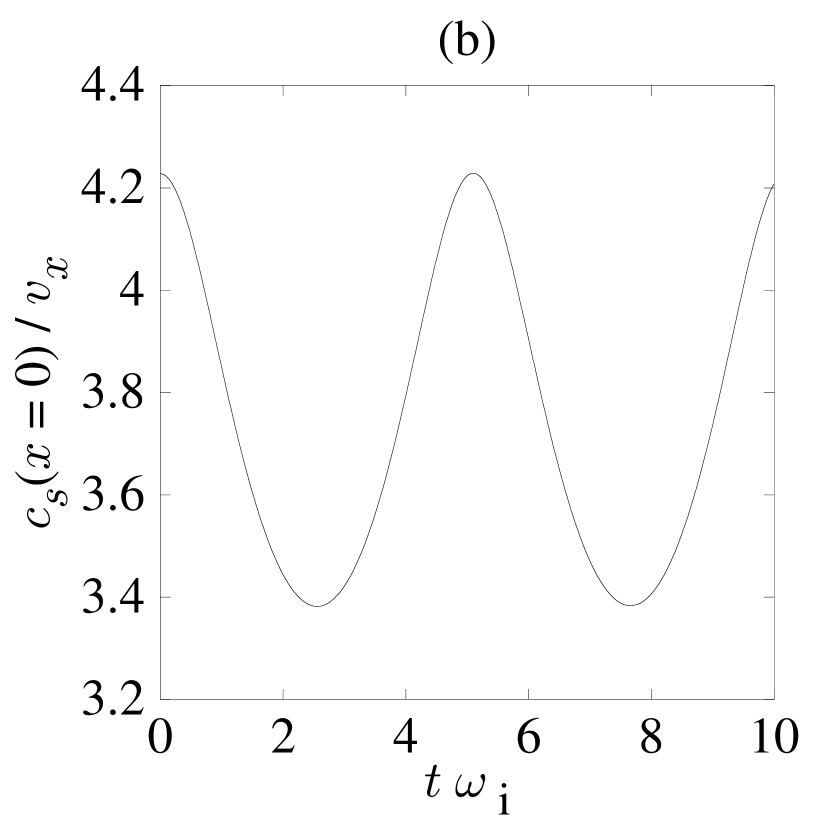
Figure 1: Dependence of the Thomas-Fermi edge $R_{\mathrm{TF}}$ (a) and the sound velocity $c_{s}=\sqrt{U_{0}n_{0}(x=0)/m}$ (b) at the center on time. Here, $a_{x}=\sqrt{\hbar/m\omega_{\mathrm{i}}}$, $v_{x}=\sqrt{\hbar\omega_{\mathrm{i}}/m}$ are the characteristic length and velocity defined by the trapping potential.

The sound velocity $c_{s}$ decreases with an increase in $R_{\mathrm{TF}}$ as shown in Fig. 1(b), also becoming periodic in time.

The decrease in the sound velocity shown in Fig. 1(b) corresponds to expansion of the analogue spacetime. We select the time at which the size of condensate becomes maximum as the final time $t_{2}$, i.e., $t_{2}:=T/2\simeq 2.55/\omega_{\mathrm{i}}$, and calculate $u_{j}^{(\lambda)}$ and $v_{j}^{(\lambda)}$ ($\lambda=1,2$). Before calculating the spectrum of the particle creation, we need to verify whether the effect of quantum backreaction can be neglected, as discussed above. Figures 2(a) and (b) show the time dependence of the total number of non-condensate particles;

$$N_{\mathrm{e}} =\int dx\>\langle\phi^{\dagger}\phi\rangle_{(1)}$$

$$=\int dx\>\sum_{j}N_{\mathrm{e}}(E_{j}^{(1)})=\int dx\>\sum_{j}|v_{j}^{(1)}|^{2},$$ (78)

and its spectrum at $t=t_{2}$. Both figures reveal that the number of Bogoliubov quasiparticles is small enough relative the number of BEC $N_{0}:=\int dx\>|\Psi|^{2}$ that the quantum backreaction will not alter the result qualitatively.

Figure 2: Dependence of the number of the Bogoliubov quasiparticles on time (a) and its spectrum (b).

Next, we investigate its particle creation. Figure 3 shows the spectrum of the particle creation $\sum_{k}|B_{jk}|^{2}$. In the low energy region $E_{j}^{(2)}<\mu$ corresponding to Fig. 3(a), the spectrum has the thermal Maxwell-Boltzmann distribution: $\sum_{k}|B_{jk}|^{2}\propto\exp(-E_{j}^{(2)}/k_{\mathrm{B}}T_{\mathrm{e}})$ with the temperature $k_{B}T_{\mathrm{e}}\simeq 0.777\hbar\omega_{\mathrm{i}}$. This result means that the spectrum of the particle creation in the analogue expanding universe obeys the thermal distribution with some temperature $T_{\mathrm{e}}$. It is widely believed that the thermal spectrum of particle creation is caused by formation of a static horizon. However, at the time $t_{2}$, there is no sonic horizon. This particle creation is quite nontrivial.

To confirm this experimentally, a BEC is needed at a temperature lower than $T_{\mathrm{e}}$ , to ensure that it is not be submerged by thermal noise. Using realistic parameters, $T_{\mathrm{e}}$ is estimated to be 5.60 nK which has been already achieved in many BEC experiments.

Figure 3: The spectrum of particle creation at $t=2.55/\omega_{\mathrm{i}}$ in the low energy region $5\hbar\omega_{i}<E_{j}^{(2)}<20\hbar\omega_{i}$ (a) and $10\hbar\omega_{i}<E_{j}^{(2)}<200\hbar\omega_{i}$ (b).

On the other hand, in the high energy region $E_{j}^{(2)}\gg\mu$ shown in Fig. 3 (b), the spectrum exhibits power-law behavior $\sum_{k}|B_{jk}|^{2}\propto E_{j}^{(2)-4}$. This power-law behavior, however, seems to be difficult to detect because particle creation in this region is very weak. In the high energy region, the modes are not hydrodynamic and the analogy breaks down. The power-law behavior might be explained by trans-Planckian physics in analogyCorley:1996ar ; Weinfurtner:2007dq .

Note that the particle creation shown in this simulation occurs spontaneously in the sense that the initial state for the excitation field has no excitation at the time just after the changing of the trapping frequency, and there is no external manipulation after the condensate starts to move. This is contrasted to the previous simulation giving homogeneous cosmological analogue Jain07 , in which the external manipulation like changing strength of the atomic interaction is required.

VI Summary

In conclusion, we have formulated quantum field theory in analogue spacetime based on the BdG equations. In this analogy, quanta in curved spacetimes are explicitly exactly related with Bogoliubov quasiparticles on condensates. It has been demonstrated that, the orthonormal relations for Bogoliubov modes correspond to that for quanta in effective spacetime with respect to the KG product. We derive a simple formula for the particle creation spectrum in terms of BdG wave functions, which can be applied to simple dynamical evolution whose initial and final condensations are quasi-static. Furthermore, we calculate the particle creation in the analogue expanding universe by numerically solving time-dependent BdG equations for an expanding BEC. The spectrum obtained is consistent with the thermal Maxwell-Boltzmann distribution for the temperature $T_{\mathrm{e}}\simeq 5.60$ nK, which is experimentally accessible. This supports the experimental testing of particle creation in an expanding universe by using a BEC.

Because we neglected the effect of the quantum backreaction from the Bogoliubov field to the BEC, we are unable to calculate the precise amount of particle creation. To overcome this deficiency, we are extending the model to incorporate the quantum backreaction and will report on this in near future. Furthermore, numerical simulations of particle creations in dynamical BEC corresponding to Hawking radiation will be reported in future studies.

Acknowledgments: MK acknowledges JSPS Research Fellowships for Young Scientists (Grant No. 207229). MT is supported in part by a Grant-in-Aid for Scientific Research from JSPS (Grant No. 18340109) and by a Grant-in-Aid for Scientific Research on Priority Areas from MEXT (Grant No. 17071008). HI is supported by a Grant-in-Aid for Scientific Research Fund of the Ministry of Education, Science and Culture of Japan (Grant No. 19540305).

References

- (1) S. W. Hawking, Nature 248, 30 (1974); S. W. Hawking, Commun. Math. Phys. 43, 199 (1975) [Erratum-ibid. 46, 206 (1976)].
- (2) W. G. Unruh, Phys. Rev. Lett. 46, 1351 (1981).
- (3) Artificial Black Holes, edited by M. Novello, M. Visser, and G. Volovik (World Scientific, 2002).
- (4) C. Barcelo, S. Liberati and M. Visser, Living Rev. Rel. 8, 12 (2005).
- (5) M. H. Anderson, J. R. Ensher, M. R. Matthews, C. E. Wieman, and E. A. Cornell, Science 269, 198 (1995).
- (6) K. B. Davis, M.-O. Mewes, M. R. Andrews, N. J. van Druten, D. S. Durfee, D. M. Kurn, and W. Ketterle, Phys. Rev. Lett. 75, 3969 (1995).
- (7) C. J. Pethick and H. Smith, Bose-Einstein Condensation in Dilute Gases (Cambridge University Press, Cambridge, 2002).
- (8) V. L. Ginzburg and L. P. Pitaevskii, Zh. Eksp. Teor. Fiz. 34, 1240 (1958) [Sov. Phys. JETP 7, 858 (1958)].
- (9) E. P. Gross, Nuovo Cimento 20, 451 (1961); J. Math. Phys. 46, 137 (1963).
- (10) L. J. Garay, J. R. Anglin, J. I. Cirac and P. Zoller, Phys. Rev. Lett. 85, 4643 (2000).
- (11) L. J. Garay, J. R. Anglin, J. I. Cirac and P. Zoller, Phys. Rev. A 63, 023611 (2001).
- (12) C. Barcelo, S. Liberati and M. Visser, Int. J. Mod. Phys. A 18, 3735 (2003) [arXiv:gr-qc/0110036].
- (13) U. Leonhardt, T. Kiss and P. Öhberg, J. Opt. B 5 S 42 (2003).
- (14) U. Leonhardt, T. Kiss and P. Öhberg, Phys. Rev. A 67, 033602 (2003).
- (15) S. Giovanazzi, C. Farrell, T. Kiss and U. Leonhardt, Phys. Rev. A 70, 063602 (2004).
- (16) S. Giovanazzi, Phys. Rev. Lett. 94, 061302 (2005).
- (17) S. Wüster and C. M. Savage Phys. Rev. A 76 013608 (2007).
- (18) Y. Kurita and T. Morinari, Phys. Rev. A 76, 053603 (2007).
- (19) R. Balbinot, A. Fabbri and S. Fagnocchi, [arXiv:0711.4520].
- (20) I. Carusotto, S. Fagnocchi, A. Recati, R. Balbinot and A. Fabbri, [arXiv:0803.0507].
- (21) S. Wüster, Phys. Rev. A 78 021601(R) (2008) [arXiv:0805.1358].
- (22) P. Jain, A. S. Bradley and C. W. Gardiner, Phys. Rev. A 76, 023617 (2007).
- (23) H. Nakano, Y. Kurita, K. Ogawa and C. M. Yoo, Phys. Rev. D 71, 084006 (2005).
- (24) S. Basak, [arXiv:gr-qc/0501097].
- (25) F. Federici, C. Cherubini, S. Succi and M. P. Tosi, [arXiv:gr-qc/0503089].
- (26) C. Barcelo, A. Cano, L. J. Garay and G. Jannes, Phys. Rev. D 74, 024008 (2006) [arXiv:gr-qc/0603089].
- (27) C. Barcelo, A. Cano, L. J. Garay and G. Jannes, Phys. Rev. D 75, 084024 (2007) [arXiv:gr-qc/0701173].
- (28) H. Takeuchi, M. Tsubota and G. E. Volovik, J. Low Temp. Phys. 150, 528 (2008).
- (29) C. Barcelo, S. Liberati and M. Visser, Int. J. Mod. Phys. D 12 1641 (2003).
- (30) C. Barcelo, S. Liberati and M. Visser, Phys. Rev. A 68 053613 (2003).
- (31) J. E. Lidsey, Class. Quant. Grav. 21, 777 (2004).
- (32) P. Jain, S. Weinfurtner, M. Visser and C. W. Gardiner, Phys. Rev. A 76, 033616 (2007).
- (33) S. Weinfurtner, P. Jain, M. Visser and C. W. Gardiner, [arXiv:0801.2673].
- (34) M. Uhlmann, [arXiv:0810.1347].
- (35) P. O. Fedichev and U. R. Fischer, Phys. Rev. Lett. 91, 240407 (2003).
- (36) P. O. Fedichev and U. R. Fischer, Phys. Rev. A. 69, 033602 (2004).
- (37) P. O. Fedichev and U. R. Fischer, Phys. Rev. D 69, 064021 (2004).
- (38) U. R. Fischer and R. Schützhold, Phys. Rev. A 70, 063615 (2004).
- (39) S. E. C. Weinfurtner, gr-qc/0404063.
- (40) M. Uhlmann, Y. Xu and R. Schutzhold, New J. Phys. 7, 248 (2005).
- (41) C. Barcelo, S. Liberati and M. Visser, Class. Quant. Grav. 18, 1137 (2001).
- (42) See, for example, A. L. Fetter and J. D. Walecka, “Quantum Theory of Many-Particle Systems” (McGraw-Hill, New York, 1971).
- (43) A. L. Fetter, Ann. Phys. (N.Y.) 70, 67 (1972).
- (44) O. Penrose, Philos. Mag. 42, 1373 (1951); O. Penrose and L. Onsager, Phys. Rev. 104, 576 (1956); C. N. Yang, Rev. Mod. Phys. 34, 694 (1962).
- (45) S. Weinfurtner, A. White and M. Visser, Phys. Rev. D 76, 124008 (2007).
- (46) See for ex. : Quantum fields in curved spaces, N. D. Birrel and P. C. W. Davies, Cambridge Univ. Press (1982).
- (47) S. Corley and T. Jacobson, Phys. Rev. D 54, 1568 (1996).