Renormalization Group Approach to Oscillator Synchronization

Abstract

We develop a renormalization group method to investigate synchronization clusters in a one-dimensional chain of nearest-neighbor coupled phase oscillators. The method is best suited for chains with strong disorder in the intrinsic frequencies and coupling strengths. The results are compared with numerical simulations of the chain dynamics and good agreement in several characteristics is found. We apply the renormalization group and simulations to Lorentzian distributions of intrinsic frequencies and couplings and investigate the statistics of the resultant cluster sizes and frequencies, as well as the dependence of the characteristic cluster length upon parameters of these Lorentzian distributions.

I Introduction

One of the most exciting aspects of modern physics is the investigation of emergent collective structures in many-body problems. Spontaneous synchronization in networks of interacting nonlinear oscillators with different (often randomly distributed) frequencies is one of the best understood collective phenomena in nonequilibrium systems Synch book Pikovsky . If the interaction between the oscillators is weak, then the oscillators will evolve in an uncoordinated fashion. In contrast, with proper connectivity and coupling strength, the population can display the same frequency as order forms. This collective behavior has been observed in diverse systems including neural networks Neural Networks1 ; Neural Networks2 ; Neural Networks3 , Josephson junctions JJ1 ; JJ2 ; JJ3 , lasers Lasers1 , electronic circuits Electronic Circuits , and a range of biological systems, including sleep cycles Sleep_Cycles , animal gaits Animal_Gaits and biological rhythms in general Biorhythms .

Useful insights into the phenomenon of synchronization are obtained by analyzing the idealized case of all-to-all coupling in the limit of a large number of oscillators. In one of the most common models each oscillator is described by a single variable, phase, that advances at a constant rate in the absence of coupling. This model is exactly soluble using a mean-field approach, and it provides a framework for understanding synchorinzation Kuramoto ; Kuramoto_review ; Acerbon's_review . In this model, above a critical coupling strength the synchronized phase appears: a finite fraction of oscillators evolve at a common frequency. Many features of this phase, such as the growth of the fraction of locked oscillators as a function of the coupling strength, can be calculated.

In many physical systems finite range interactions are a more realistic description. The simplest of these interactions are nearest neighbor couplings JJ4 ; Lasers2 . In general, finite range coupled systems are much harder to analyze, and, as a result, there are few theoretical tools that produce a quantitative description of the collective motion. Much of our understanding of these systems rests on numerical solutions of the governing equations. We propose an alternative method to attack the synchronization problem. The method we develop is a real-space renormalization group (RG) designed to work well on systems with strong randomness, where both the intrinsic oscillation frequencies and coupling constants are random variables taken from distributions with long tails. The specific example we investigate contains Lorentzian distributions. This method is shown to be accurate in systems with short range interactions.

In this paper, we analyze a one dimensional chain of oscillators interacting with their nearest neighbors. Despite the relative simplicity of the model, it can exhibit complex behavior since randomness competes with a tendency to establish macroscopic order. This system is below the lower critical dimension for a synchronization transition (Strogatz and Mirollo Strogatz and Mirollo 1 ; Strogatz and Mirollo 2 showed that a nearest-neighbor chain cannot exhibit extensive synchronization), and therefore can not be analyzed with mean-field techniques. Collective behavior still arises, albeit at a finite length scale: the chain becomes fragmented into finite length clusters of coherently moving oscillators. We are interested in the distribution of cluster lengths, cluster frequencies, and how these change as a function of the coupling strengths and bare frequencies. Additionally, we seek to develop a renormalization group scheme that will allow us to predict with some accuracy the individual local behavior of oscillators. We also carry out an extensive numerical study of the problem and use it as a benchmark for comparison with the RG.

The paper is organized as follows. In Sec. II we outline the strong disorder renormalization group approach with the details of the steps for the nearest-neighbor oscillator chain derived in Sec. II.1. In Sec. III, we compare some key statistical features of the cluster state obtained by the RG with results from direct numerical simulations of the equations of motion. In Sec. IV we outline our findings concerning the physics of the synchronized clusters, presenting results for the distributions of cluster sizes, cluster frequencies, as well as the dependence of the characteristic length scale of the clusters on the widths of the coupling and frequency distributions. Concluding remarks are made in the last section.

II Strong Disorder Renormalization Group

To analyze the random oscillator chain we develop a strong-disorder real space RG technique. A similar method has been used successfully in quantum mechanical systems to analyze the ground state of the random Heisenberg model MaDas79 ; MaDas80 ; DSF94 ; DSF98 , and the superfluid-insulator transition in random bosonic chains AKPR04 ; AKPR08 (a quantum reactive analog of the nearest-neighbor chain, where the $\ddot{\theta}$ replaces $\dot{\theta}$, and $\theta$ is a quantum operator).

The main idea behind the strong disorder approach applied to the quantum-mechanical problem is best demonstrated in the case of the spin-1/2 Heisenberg model:

$$\hat{H}=\sum\limits_{i}J_{i}\hat{\bf S}_{i}\cdot\hat{\bf S}_{i+1}.$$ (1)

The $i$’th term in the sum considered on its own, splits the four states of the spins $i$ and $i+1$, into a singlet state, and three triplet states excited by the energy $J_{i}$. Thus a real-space decimation step can be proposed. First, freeze the spin pair with the strongest interaction, $J_{n}=\text{max}\{J_{i}\}$, into a singlet state. Perturbative corrections to this state introduce an effective coupling between the neighbors of the spins $n$ and $n+1$ which is:

$$H_{RG}=\frac{J_{n-1}J_{n+1}}{2J_{n}}\hat{\bf S}_{n}\cdot\hat{\bf S}_{n+1},$$ (2)

an interaction identical in form to the operators in the bare Hamiltonian, but with a much suppressed strength: $J_{eff}=\frac{J_{n-1}J_{n+1}}{2J_{n}}<J_{n-1},\,J_{n},\,J_{n+1}$. By repeating this decimation step, the number of free spins is gradually decreased; at the stage when all spins are bound into singlets, we obtain the ground state of the Hamiltonian.

The decimation step described above is justified if the coupling to the rest of the chain is much weaker then between the two spins in question. This is guaranteed if the chain considered has broad coupling distributions. Below, we use a real-space renormalization group approach to analyze the nearest-neighbor oscillator chain with broad disorder distributions.

The nearest-neighbor oscillator chain presents a classical problem with dissipative equations of motion, rather than a quantum problem with a conserved Hamiltonian. Nevertheless, we can develop an analogous strong disorder RG method for this problem as well. The chain is governed by the equations of motion

$$\dot{\theta}_{i}=\omega_{i}+K_{i-1}\sin{(\theta_{i-1}-\theta_{i})}+K_{i}\sin{(\theta_{i+1}-\theta_{i})},$$ (3)

where $\theta_{i}$ is the phase of the $i$th oscillator. The $\omega_{i}$ are the intrinsic frequencies taken from a random distribution (we assume zero mean without loss of generality) and the $K_{i}$ give the couplings to the nearest neighbors also taken from a random distribution. The coupling will organize the oscillators into clusters of common frequency $\bar{\omega}$ defined as

$$\bar{\omega}_{i}\equiv\lim_{(t-t_{0})\rightarrow\infty}\frac{\theta_{i}(t)-\theta_{i}(t_{0})}{t-t_{0}},$$ (4)

such that each oscillator in a given cluster shares its $\bar{\omega}$ with all the other oscillators in the same cluster. We seek to understand the statistics of the cluster sizes and frequencies.

The renormalization group approach is based on two observations. A strong coupling between two oscillators tends to force them to rotate at the same frequency forming a cluster that we can then treat as a single effective oscillator. Concomitantly, oscillators with anomalously large frequencies rotate essentially independently, with little effect from their neighbors. These ideas lead to two decimation steps: a strong coupling decimation and a fast oscillator decimation. We apply these steps iteratively, sweeping through the oscillators from large values of $\omega_{i}$ and $K_{i}$ to smaller values.

II.1 Decimation steps

As in the case of the quantum Heisenberg chain, our real space RG will be carried out iteratively by treating at each step the strongest term in the right-hand-side of the equations of motion, i.e., the term with the highest frequency. In the oscillator chain the strongest term at each step could be either a strong coupling $K_{i}$, or a large frequency, $\omega_{i}$. Let us now derive the appropriate decimation steps for the nearest-neighbor chain for these two cases. We begin by slightly generalizing the model to

$$m_{i}\dot{\theta}_{i}=m_{i}\omega_{i}+K_{i-1}\sin{(\theta_{i-1}-\theta_{i})}+K_{i}\sin{(\theta_{i+1}-\theta_{i})},$$ (5)

where a new parameter $m$ is added. It will follow from the strong coupling decimation step defined below that when two oscillators with $m_{i}$ and $m_{i+1}$ are described by one effective oscillator, its $m$ is given simply by $m_{i}+m_{i+1}$. Hence, the value of $m$ represents the number of original oscillators that this effective oscillator represents. It will become apparent that oscillators with larger $m$ are less affected by perturbations from their neighbors, so $m$ is a measure of the inertia of an oscillator and will be referred to as its “mass”, although it is not a true mass or inertia in the sense of Newton’s second law.

II.1.1 Strong coupling decimation

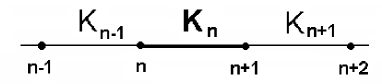
Figure 1: A small piece of the chain around the strongest coupling, labeled here as $K_{n}$. All the neighboring $K_{i}$ and all the local $\omega_{i}$ are assumed to have much smaller magnitude then $K_{n}$.

The phases of two oscillators connected by a very large coupling tend to advance in synchrony. The strong coupling step replaces this pair of oscillators by a single effective oscillator with a different mass and frequency determined as follows. Consider the largest coupling in the chain: suppose this coupling is $K_{n}$, Fig. 1. Because of the strong disorder the frequencies $\omega_{n},\omega_{n+1}$ of the pair of oscillators that $K_{n}$ couples and the couplings $K_{n-1},K_{n+1}$ to the neighbors of the pair will almost always be small compared to $K_{n}$. Ratios such as $\omega_{n}/K_{n},K_{n-1}/K_{n}$, are therefore expected to be small numbers; we will use a symbol $\epsilon$ to denote quantities of this order. For small $\epsilon$, $K_{n}$ will couple oscillators $n$ and $n+1$ into a synchronized cluster that can be represented as a single effective oscillator described by phase $\Theta$

$$\Theta\equiv(m_{n}\theta_{n}+m_{n+1}\theta_{n+1})/M,$$ (6)

possessing mass $M$,

$$M=m_{n}+m_{n+1},$$ (7)

and an effective intrinsic frequency $\Omega$,

$$\Omega=(m_{n}\omega_{n}+m_{n+1}\omega_{n+1})/M.$$ (8)

We refer to such pair of oscillators strongly coupled (cf.  and Sec. II.2).

The small frequency difference $\omega_{n+1}-\omega_{n}$ and the small couplings $K_{n-1}$ and $K_{n+1}$ induce a small phase difference $\delta\equiv\theta_{n+1}-\theta_{n}$ between the two oscillators. Using $\theta_{n}=\Theta-m_{n+1}\delta/M$ and $\theta_{n+1}=\Theta+m_{n}\delta/M$, Eqs. (5) gives the evolution equation for the phase of the new effective oscillator

$$M\dot{\Theta}=M\Omega + K_{n-1}\sin{(\theta_{n-1}-\Theta+\frac{m_{n+1}}{M}\delta)}$$ (9)

$$+ K_{n+1}\sin(\theta_{n+2}-\Theta-\frac{m_{n}}{M}\delta).$$

There are corresponding equations for $\dot{\theta}_{n-1}$ and $\dot{\theta}_{n+2}$. Aside from the new $\delta$-terms, the equations take the original form.

There are two contributions to the phase $\delta$. The contribution from the frequency difference is a time independent phase given to leading order in $\epsilon$ by

$$\delta_{0}=\frac{\mu_{n,n+1}}{K_{n}}(\omega_{n+1}-\omega_{n}).$$ (10)

where $\mu_{i,j}^{-1}=m_{i}^{-1}+m_{j}^{-1}$ is the reduced mass. This can be seen by considering just the two oscillators coupled by the strong $K_{n}$ and disregarding effects of the rest of the chain. Then, as can be seen from the difference of their equations of motion, Eqs. (5), as long as $\omega_{n+1}-\omega_{n}$ is smaller then $K_{n}/\mu_{n,n+1}$, which will be the case if $K_{n}$ is much larger then all the neighboring parameters, these two oscillators will reach a state in which they rotate at the same frequency and are separated by the fixed phase difference $\delta_{0}$. We will see this explicitly after writing down an equation of motion for $\delta$ below. For the one dimensional chain we can redefine $\theta_{n-1}$ and prior phases, as well as $\theta_{n+2}$ and subsequent phases, to absorb such constant phases, and so we may ignore them. This maneuver is restricted to one dimension in the spatial lattice, and the extension of the method to higher dimensions would require a more careful study of the effect of these additional phases.

The couplings $K_{n-1}$ and $K_{n+1}$ to the neighbors of the pair give an additional contribution to $\delta$ that is time dependent as the neighboring oscillators evolve. To leading order in $\epsilon$ it turns out that these oscillating corrections give small extra coupling terms of forms not included in the equation of motion Eqs. (5): a second nearest neighbor interaction between oscillators, a three body interaction involving the new effective oscillator and the neighboring pair, and a second harmonic correction to the form of the pairwise interaction. The detailed forms of these terms can be found in Oleg_Thesis . We will neglect these more complicated interaction terms since they are much weaker then all other competing interactions.

These results are derived from the exact expression for the equation of motion of the phase difference $\delta(t)$,

$$\dot{\delta} =-\frac{K_{n}}{\mu_{n,n+1}}\sin{\delta+(}\omega_{n+1}-\omega_{n})$$

$$+\frac{K_{n+1}}{m_{n+1}}\sin{\left(\theta_{n+2}-\Theta-\frac{m_{n}}{M}\delta\right)}$$

$$+\frac{K_{n-1}}{m_{n}}\sin{\left(\theta_{n-1}-\Theta+\frac{m_{n+1}}{M}\delta\right)}.$$ (11)

This equation describes a damped particle in a time dependent washboard potential. The relaxation rate $K_{n}/\mu_{n,n+1}$ given by the first term on the right hand side is fast compared with the other terms in the equation. The solution can therefore be developed as an expansion in a ratio of time scales, and the leading order term is the adiabatic solution

$$\delta\simeq\frac{\mu_{n,n+1}}{K_{n}}\left[(\omega_{n+1}-\omega_{n})+\frac{K_{n+1}}{m_{n+1}}\sin{\left(\theta_{n+2}-\Theta\right)}\right.\\ +\left.\frac{K_{n-1}}{m_{n}}\sin{\left(\theta_{n-1}-\Theta\right)}\right].$$ (12)

The first term in the braces gives the constant phase $\delta_{0}$, and on substituting back into Eq. (9) and expanding to first order in small $\delta$, the second and third terms give the corrections to the interaction terms that we will neglect, as discussed above. Specifics of the calculations outlined in this section are presented in Oleg_Thesis .

In summary, the effect of the strong coupling decimation step is to replace the pair of oscillators with phases $\theta_{n}$ and $\theta_{n+1}$ by a single oscillator with phase $\Theta$, mass $M$ and frequency $\Omega$ given by Eqs. (6), (7), and (8).

II.1.2 Fast oscillator decimation

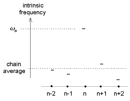
Figure 2: A small piece of the chain around the oscillator with the largest frequency, labeled here as $\omega_{n}$. All the neighboring $K_{i}$ and all the neighboring $\omega_{i}$ are assumed to have much smaller magnitude then $\omega_{n}$.

Next we consider the case where the highest frequency scale in the problem is a bare frequency. In this case we apply the notion that the phase of an oscillator with frequency much different from its neighbors tends to advance as if the oscillator were decoupled. Consider the oscillator with the largest frequency in the entire chain: suppose this is oscillator $n$ with intrinsic frequency $\omega_{n}$, Fig. 2. Because of strong disorder the coupling strengths $K_{n-1}$ and $K_{n}$ to the neighboring oscillators and the frequencies $\omega_{n\pm 1}$ of these oscillators will almost always be small compared to $\omega_{n}$. Therefore we expect ratios such as $K_{n-1}/\omega_{n}$ and $\omega_{n-1}/\omega_{n}$ to be small compared to 1; as before we denote quantities of this order by $\epsilon$. To zeroth order in $\epsilon$ the $n$’th oscillator runs freely, with the frequency $\omega_{n}$. We call such oscillators “fast oscillators” (see and Sec. II.2 for elaboration).

Deviations from the free-running solution can be calculated perturbatively in $\epsilon$. The most important effect we might look for is an induced effective coupling via oscillator $n$ between the neighbors $n-1$ and $n+1$, since this might lead to their synchronization. However, at least to order $\varepsilon^{2}$ as we describe below, we find that there is no induced interaction that tends to lock the neighboring oscillators . Thus the main effect of decimating the largest frequency oscillator in the chain is to eliminate this oscillator from further consideration (it represents a cluster in the final tally at frequency close to $\omega_{n}$ and with a size given by its mass parameter $m$) and to cut the chain into two pieces. This is a key feature of the strongly random chain that limits the size of synchronized clusters. At order $\epsilon^{2}$ we do find a renormalization of the frequencies of both the eliminated oscillator and the two neighbors remaining in the chain.

We now investigate the perturbation of the motion of the fast oscillator (oscillator $n$ in Fig. 2) given by Eqs. (5). To zeroth order in $\epsilon$, the solution to $\theta_{n}$ is given by the uniform running state $\theta_{n}=\omega_{n}t$. There are two $O(\epsilon^{2})$ effects that slightly perturb the average rate of this uniform advancement of the phase. The first is the fact that oscillator $n$ rotates in the tilted washboard potential created by its neighbors. Since typically $\omega_{n-1},\omega_{n+1}\ll\omega_{n}$ for strong disorder, this potential can be treated as effectively static. The second effect is a small component of fast dynamics added to the motion of the neighboring oscillators, which then acts back on oscillator $n$. Both of these effects change the average frequency of the eliminated oscillator by a shift of order $\epsilon^{2}$. There are corresponding corrections to the motion of the neighboring oscillators as well. These effects will be apparent in the following analysis.

First, consider the motion of $\theta_{n}$ in the nearly static washboard potential from the neighbors, calculated to second order in the coupling. Setting the neighboring phases in Eqs. (5) to fixed values $\theta_{n\pm 1}^{(0)}$ gives the oscillation period of the $n$th oscillator.

$$T_{n}=\int_{0}^{2\pi}\frac{d\theta_{n}}{\omega_{n}+\frac{K_{n-1}}{m_{n}}\sin{(\theta_{n-1}^{(0)}-\theta_{n})}+\frac{K_{n}}{m_{n}}\sin{(\theta_{n+1}^{(0)}-\theta_{n})}}.$$ (13)

Expanding the denominator and performing the integration over $\theta_{n}$ gives the change to the frequency of the $n$th oscillator $\bar{\omega}_{n}-\omega_{n}$ with $\bar{\omega}_{n}=2\pi T_{n}^{-1}$

$$\delta\bar{\omega}_{n}^{(1)}\simeq-\frac{K_{n-1}^{2}}{2m_{n}^{2}\omega_{n}}-\frac{K_{n}^{2}}{2m_{n}^{2}\omega_{n}}-\frac{K_{n-1}K_{n}}{m_{n}^{2}\omega_{n}}\cos{(\theta_{n+1}^{(0)}-\theta_{n-1}^{(0)})}.$$ (14)

The second effect perturbing the motion of the fast oscillator arises from the rapid induced motion of the neighboring oscillators $\theta_{n\pm 1}\simeq\theta_{n\pm 1}^{0}+\delta\theta_{n\pm 1}$. For example from Eqs. (5) for oscillator $n-1$ we have

$$\delta\theta_{n-1} \simeq\frac{K_{n-1}}{m_{n-1}}\int dt~{}\sin{(\omega_{n}t-\theta_{n-1}^{0})}$$ (15)

$${=}{-}\frac{K_{n-1}}{m_{n-1}\Omega}\cos{(\omega_{n}t-\theta_{n-1}^{0}),}$$ (16)

where we use the zeroth order solution for oscillator $n$ and the influence of the next nearest neighbor $\theta_{n-2}$ only appears at higher order. This provides a perturbation back on the $n$th oscillator given by expanding the second term on the right hand side of Eqs. 5 for $i=n$ to first order in $\delta\theta_{n-1}$

$$\delta\dot{\theta}_{n}\simeq\frac{K_{n-1}}{m_{n}}\cos{(\omega_{n}t-\theta_{n-1}^{0})}\delta\theta_{n-1}.$$ (17)

Using Eq. (15) for $\delta\theta_{n-1}$, averaging over the fast oscillations, and adding the similar effect from oscillator $n+1$ gives the change in the average frequency of the $n$th oscillator

$$\delta\bar{\omega}_{n}^{(2)}\simeq-\frac{K_{n-1}^{2}}{2m_{n}m_{n-1}\omega_{n}}-\frac{K_{n}^{2}}{2m_{n}m_{n+1}\omega_{n}}.$$ (18)

Combining Eqs. (14) and (18) gives the total renormalization of the frequency of the fast oscillator to second order

$$\delta\bar{\omega}_{n}\simeq-\frac{K_{n-1}^{2}}{2m_{n}\mu_{n,n-1}\omega_{n}}-\frac{K_{n}^{2}}{2m_{n}\mu_{n,n+1}\omega_{n}}\\ -\frac{K_{n-1}K_{n}}{m_{n}^{2}\omega_{n}}\cos{(\theta_{n+1}-\theta_{n-1})},$$ (19)

with $\mu_{i,j}^{-1}=m_{i}^{-1}+m_{j}^{-1}$ as before.

There are reciprocal effects on the neighboring oscillators that can be calculated by a similar procedure. Since at the pairwise level interactions between the oscillators conserve the mass-weighted frequency average , we can immediately see that the first two terms in Eq. (19) correspond to frequency renormalizations of the neighboring oscillators

$$\delta\bar{\omega}_{n-1}=\frac{K_{n-1}^{2}}{2m_{n-1}\mu_{n,n-1}\omega_{n}},\ \delta\bar{\omega}_{n+1}=\frac{K_{n}^{2}}{2m_{n+1}\mu_{n,n+1}\omega_{n}}.$$ (20)

The fact that the first two frequency correction terms in Eq. (19) are additive suggests that they can be obtained from the analysis of a pair of 2-oscillator systems. This calculation can be performed exactly for the phase difference, for example $\phi=\theta_{n}-\theta_{n-1}$. Such a frame independent analysis reproduces at $O(\epsilon^{2})$ the first two terms in Eq. (19) and the terms in Eq. (20) which were obtained in the specific reference frame of the average frequency, but also yields terms that are higher order in $\epsilon$. In the context of the full chain including these higher order terms is an uncontrolled approximation, however empirically we find them to produce a better match with the simulation data in some rare cases. Hence, in the numerical renormalization of the chain, we employ the expressions produced by this analysis.

The phase difference of oscillators $n$ and $n-1$ isolated from the rest of the chain satisfies

$$\dot{\phi}=(\omega_{n}-\omega_{n-1})-\frac{K_{n-1}}{\mu_{n,n-1}}\sin{\phi}.$$ (21)

A period $T$ over which this phase difference grows by $2\pi$ can be defined analogously to Eq. (13), but since there is only one sine term, the integral can be computed analytically. From that solution and the fact that for the isolated pair $m_{1}\dot{\theta}_{1}+m_{2}\dot{\theta}_{2}=m_{1}\omega_{1}+m_{2}\omega_{n}$ we obtain the correction to the frequency of oscillator $n$ coming from oscillator $n-1$:

$$\delta\bar{\omega}_{n,n-1}=\\ \frac{\mu_{n,n-1}(\omega_{n-1}-\omega_{n})}{m_{n}}\left[1-\sqrt{1-\left(\frac{K_{n-1}}{\mu_{n,n-1}(\omega_{n}-\omega_{n-1})}\right)^{2}}\right].$$ (22)

We use this expression to replace the first term on the right hand side of Eq. (19) with a corresponding expression for the first term in Eq. (20), and similar expressions for the second pair of terms.

The new cosine interaction term in Eq. (19) also warrants discussion. There is a corresponding renormalization of the equations of motion of each of its neighbors. In the motion of the fast oscillator Eq. (19), we ignore the cosine term since it averages to zero on the long time scale of the period of oscillators $n\pm 1$. In the equations for $\dot{\theta}_{n-1}$and $\dot{\theta}_{n+1}$ the corresponding term is a coupling $\propto\cos{(\theta_{n+1}-\theta_{n-1})}$ between these oscillators, with the same sign in the equations of motion of both neighboring oscillators. Therefore this interaction does not have action-reaction symmetry. This sign peculiarity arises because the decimated oscillator has a particular direction of rotation. Because of the lack of action-reaction symmetry, the cosine term does not tend to pull neighboring oscillators together, and so does not directly influence the clustering. We therefore omit this term in the renormalization procedure.

II.2 Implementation

The chain of oscillators is renormalized by successive application of the two decimation steps developed above. These are executed numerically on a list of parameters $(m_{i},\omega_{i},K_{i})$ representing the chain of oscillators. A single decimation step consists of finding the largest frequency of the set $\left\{\omega_{i},\frac{K_{i}}{2\mu_{i,i+1}}\right\}$, renormalizing the appropriate term as described above, and working down to smaller ones later. Notice that it is the largest $\frac{K_{i}}{2\mu_{i,i+1}}$ that identifies the pair of oscillators to be subjected to the strong coupling step, not the largest $K_{i}$. The reason for this becomes clear when all equations are divided by their respective $m_{i}$. An equation for the phase difference $\theta_{i+1}-\theta_{i}$ contains the term $\frac{K_{i}}{\mu_{i,i+1}}\sin{(\theta_{i+1}-\theta_{i})}$. When $\frac{K_{i}}{\mu_{i,i+1}}$ is much larger then the terms representing coupling to the neighbors, this phase difference will tend to be locked and the strong coupling step should be applied to the pair of oscillators $i$ and $i+1$. The factor of $2$ was used in the denominator to make sure that the initial stages of the RG procedure, couplings and frequencies are treated on equal footing.

Initial values of masses are all set to $1$. The numerical procedure identifies the oscillators with $\omega$ and $K$ that lie in a narrow band of magnitudes at the top of the spectrum of remaining values, and then decimates those oscillators according to the steps defined in Sec.s II.1.1 and II.1.2. A band is used, rather than just selecting the largest values, to improve the efficiency of the code. The width of the band is chosen to be narrow ($1\%$ of the chain) to maintain the descending order in $\omega$ and $K$ for the decimation of nearby oscillators. Oscillators decimated in the fast oscillator step form a cluster in the final tally, with the effective mass describing the size of the cluster and the frequency giving the time-averaged rate at which the phase of this cluster advances. As described in Sec. II.1.2, these oscillators are removed from the chain. After the decimation of oscillator band, the remainder of the chain consists of fewer oscillators, which have lower coupling strengths and frequencies within a narrowed spectrum. The procedure is then repeated for successively lower bands of $K$ and $\omega$.

During the RG execution, two types of special cases related to violations of the assumptions based on strong disorder are occasionally encountered. First, in our treatment of the oscillator with the largest $\omega$ we have made an assumption that nearby $\omega$ and $K$ are small in comparison. This assumption defines the physical content of the strong disorder assumption. In real chains, it is possible to have neighbors with parameters which are somewhat lower yet the difference is not large enough to guarantee that effects of these neighbors are small. This is especially important as the spectrum of the remaining $K$ and $\omega$ values shrinks. To be more precise, for a decimation of a fast oscillator $n$, the magnitude of $r_{FO}$ defined by

$$r_{FO}\equiv\mathrm{Max}\left[\frac{K_{n}}{\mu_{n,n+1}|\omega_{n}-\omega_{n+1}|},\frac{K_{n-1}}{\mu_{n,n-1}|\omega_{n}-\omega_{n-1}|}\right]$$ (23)

determines whether the effects of the neighbors are small, so that the step can be performed. Similarly, for a strong coupling decimation of oscillators $n$ and $n+1$, the magnitude of the ratio

$$r_{SC}\equiv\frac{K_{n}}{\mu_{n,n+1}|\omega_{n}-\omega_{n+1}|}$$ (24)

determines whether the step should be performed. In our implementation of the RG we set set the criteria to $r_{FO}<1$ and $r_{SC}>1$. This choice was based on the numerical study of small chains ($N<10$) as well as on the fact that for sinusoidal coupling $r_{FO}$ does not need to be very small for $\omega_{n}t$ to give a good approximation to the dynamics of the $n$th oscillator. This is hinted by the square-root dependence of the frequency correction in Eq. (22): analysis of that formula indicates that $\bar{\omega}_{n}$ quickly approaches $\omega_{n}$ as $r_{FO}$ decreases below $1$. A more thorough discussion of the choice for $r_{FO}$ and $r_{SC}$ can be found in Oleg_Thesis .

There is a second type of violation of the assumptions based on the strong disorder. Note that single oscillators with $m=1$ or oscillators representing clusters with $m>1$ are normally subjected to the fast oscillator decimation step at some point in the RG procedure: most of the bare oscillators either join other oscillators in building clusters, which are eventually decimated via the fast oscillator step, or they are decimated as fast oscillators directly without undergoing a strong coupling step. But some rare combinations of frequencies and couplings will prevent the decimation from occurring at all within this scheme. For example, while an oscillator’s frequency may lie in the executable band, this oscillator may be coupled via a $K$ which is outside this band (it has a somewhat lower magnitude), but may nevertheless cause $r_{FO}$ to exceed $1$. In general, when the RG reaches the scale of that coupling, it will perform a strong coupling decimation step. However, in rare cases this may not happen due to intervening steps that have modified the neighboring parameters, rendering that coupling no longer strong according to the $r_{SC}$ criterion. As a result, the site in question has not been subjected to either decimation step. To address such unusual cases, the algorithm sweeps repeatedly through the entire spectrum of $\omega$ and $K$ values until nothing is left to decimate.

III Numerics

While the discussion above constructed a general RG algorithm, let us now explore the scheme within a disorder realization with a specific class of frequency and coupling distributions $g(\omega),\,G(K)$. The bare frequencies in the system we analyze have a symmetric Lorentzian distribution with a cutoff:

$$g(\omega)=\frac{C_{1}}{1+\omega^{2}},$$ (25)

with $-\omega_{c}\leq\omega\leq\omega_{c}$. The couplings are positive and are taken from a half Lorentzian with a cutoff:

$$G(K)=\frac{2\mu C_{2}}{\mu^{2}+K^{2}}$$ (26)

with $0\leq K\leq K_{c}$. The cutoffs are used to facilitate the effective numerical simulations (Sec. III.2 below): increasing cut-off values increases the time needed for simulations. The same cut-off values for $\{\omega\}$ and $\{K\}$ were chosen: $\omega_{c}=K_{c}=100$; the values of these cutoffs are much larger then the FWHM of all Lorentzians that we considered. The $C_{1}$ and $C_{2}$ are normalization constants that become $1/\pi$ when the cut-off values $\omega_{c}$ and $K_{c}$ are infinite. Notice that due to the structure of Eqs. (5), it is always possible to divide all equations by a constant such that the width of one of these distributions will be unity: this only changes the time scale of all the processes in the chain. We chose $g(\omega)$ to have unity width and explore the physics by varying the other width parameter $\mu$.

III.1 Renormalization group

The RG procedure is applied to a chain of $10^{6}$ oscillators. Twelve values of coupling width $\mu$ are studied: $\mu=0.025$, $0.05$, $0.25$, $0.5$, $0.625$, $1.25$, $2.5$, $3.75$, $4.5$, $5$, $6.25$, and $7.5$. The set of random numbers defining the particular realizations of the chain were different in the RG and in the simulations (below) for the statistical comparisons, but were identical for the real-space comparison described in Sec. III.3.

III.2 Simulations

In order to explore both the system’s characteristics and the reliability of the renormalization group, Eqs. (3) are also integrated numerically. The numerical method is a variable stepping Runge-Kutta algorithm. Systems of $N=10000$ oscillators are solved with $N$ intrinsic frequencies chosen randomly from the cutoff distribution given by Eq. (25). Similarly, $N-1$ coupling constants are randomly selected from the cutoff distribution given by Eq. (26). The same twelve values of coupling width $\mu$ that are used in the RG are studied in the simulations. Results for each value of $\mu$ are averaged over $100$ realizations of the intrinsic frequencies and coupling constants. To help facilitate comparisons between different distribution widths the same 100 random number seeds are used for each distinct coupling width.

The simulations are performed for a relatively long time of $t=10000$. Running phases at each site are recorded at regular intervals and used to calculate average frequencies over a time $T$ according to

$$\bar{\omega}_{i}(T)=\frac{\theta_{i}(t_{0}+T)-\theta_{i}(t_{0})}{T};$$ (27)

with $T=t-t_{0}$ [compare with the theoretical definition of $\bar{\omega}$ given by Eq. (4)]. The time $t_{0}$ is chosen to eliminate transients: increasing values are tried until average frequencies remain unchanged. In these simulations, the value of $2\pi/T$ sets the resolution limit in $\bar{\omega}_{i}$ to distinguish two neighboring frequency clusters. A group of oscillators is determined to be members of a synchronized cluster only if all the members ($i=n,n+1,\ldots,n+m+1$) have the same value of $\bar{\omega}_{i}$ as the neighboring sites within some tolerance $\left|\bar{\omega}_{\ell}-\bar{\omega}_{i}\right|\leq\eta$ $(\ell=i-1$ and $i+1)$. Since $T^{-1}$ is $O\left(10^{-4}\right)$ the tolerance $\eta$ is set to $10^{-3}$.

III.3 Comparison of RG and simulations.

While we are primarily interested in correctly capturing the statistical characteristics through RG, the local validity of our procedure can be established by comparing the frequency cluster structure that it predicts with results from the simulations. Figure 3 plots these comparisons over a representative sample of 150 oscillators from chains of $N=10000$ at 3 different coupling distribution widths.

Figure 3: Comparisons between cluster structure of dynamic frequencies found in numerical simulations of a 10000-oscillator chain with those predicted by RG over a representative number of lattice sites. The top row (a-c) plots the dynamic frequencies found for 500 oscillators in the simulations and demonstrate how some oscillators maintain large frequencies. The dashed boxes in the centers of (a-c) encircle 50 oscillators magnified in panels (d-f), respectively. In (d-f) average frequencies from simulations given by Eq. (27) are denoted by solid squares, while RG predictions are shown as open circles. The differences between RG and simulations are shown in panels (g-i). Each column shows results for a different coupling width: $\mu=1.25$ (a,d,g), $\mu=3.75$ (b,e,h), and $\mu=7.5$ (c,f,i).

For all 3 values of $\mu$, there are clusters with large frequency oscillators interspersed. As expected, the characteristic size of these clusters grows with $\mu$. There is excellent agreement of the cluster sizes, locations, and frequencies between the two approaches. This provides some confidence that the essential mechanisms are captured by the RG procedure.

Analysis of these and similar plots, shows that the agreement of the cluster frequencies becomes more accurate with increasing cluster size. The reason for this result is the smaller boundary-to-bulk ratio of larger clusters, which is more apparent if Eqs. (5) is rewritten as

$$\dot{\theta}_{i}=\omega_{i}+\frac{K_{i-1}}{m_{i}}\sin{(\theta_{i-1}-\theta_{i})}+\frac{K_{i}}{m_{i}}\sin{(\theta_{i+1}-\theta_{i})}$$ (28)

As clusters become larger, the importance of the coupling to the rest of the chain is weighted down by a $1/m$ factor. In the fast oscillator decimation, this is manifested by the appearance of this factor in the frequency correction. Also, when a cluster is built up by a strong coupling decimation step, any frequency renormalizations of the component oscillators by prior fast oscillation decimation steps cancel when the weighted sum of the frequencies is calculated to give the frequency of the new cluster. Thus the cluster frequencies $\bar{\omega}_{i}$ are given to a good approximation by the average of the constituent bare $\omega$ values, plus the small correction due to the fast oscillator decimation step that yields the final cluster.

Investigating the frequency distribution of clusters of a given size provides further insight into the validity of this RG procedure.

Figure 4: Number of clusters of a particular frequency divided by the total length of the chain ($N=10^{6}$). The plot compares the RG prediction (solid lines) and the simulation results (open diamonds) for 3 coupling widths and 4 cluster sizes. Each panel has a fixed coupling width and cluster size. Frequencies, on the hortizontal axes, are grouped into bins of size $\Delta\bar{\omega}=0.1$. The rows are each a different cluster size; $m=1$ (a-c), $2$ (d-f), $3$ (g-i), and $4$ (j-l) from top to bottom. Each column is a different coupling width: $\mu=1.25$ left, $\mu=3.75$ center, and $\mu=7.5$ right.

This is shown in Fig. 4, where for each cluster size $m$ from 1 to 4, the RG predictions are compared with the results from simulations using three values of the parameter $\mu$. The two methods are in excellent agreement for the larger values of $m$ and also for all $m$ at small values of $\mu$.

The comparisons in Fig. 4 show a small but systematic underestimation of the number of smallest sized clusters ($m=1$ and $m=2$) near zero frequency and large coupling [panels (b) and (c) and less so in in panels (e) and (f)]. The rms difference between the RG generated and numerically calculated curves ranges between $0.7-2.2\cdot 10^{-4}$, with the worst agreement in panel (b), and best agreement in panel (l). The region of the greatest discrepancy, small $m$ and $\omega$, is in fact where the fast oscillator decimation is expected to be least accurate, since by the time the RG sweep reaches these frequencies, the distributions of remaining frequencies and couplings are no longer expected to be wide so that the approximations based on strong randomness are not as accurate. However the disagreement decreases with increasing $m$, because, as described above, the frequencies of larger clusters are insensitive to the corrections from neighbors.

IV The unsynchronized phase of an oscillator chain

Let us now use the results of the RG and the simulations to discuss the statistical properties of the frequency clustering in the one dimensional oscillator chain with strong randomness.

IV.1 Cluster size distribution

The main measurable physical quantity that arises in our analysis is the distribution of cluster sizes. In Fig. 5 we show the distribution of cluster sizes for several widths $\mu$ of the coupling distribution from the RG and simulations. The RG was performed on one single realization of $10^{6}$ oscillators, while the simulations were performed on $100$ realizations of $10^{4}$ oscillator chains. Since the characteristic cluster size is much smaller then $10^{4}$, we combine results from all $100$ realizations and analyze them as a single chain of size $10^{6}$. As can be seen in Fig. 5, good agreement exists between the RG and the simulations. The apparent discrepancies at the largest cluster sizes are due to statistical fluctuations resulting from the small number of such clusters present in the $10^{6}$ oscillator ensemble.

Figure 5: Number of clusters over a range of sizes. The plot compares RG predictions (open circles) with numerical integrations of Eqs. (5) (solid squares). The curves are spread out for clarity by multiplying each successive data set as $\mu$ increases by $0.1$ (a linear shift in the semilog plot). The solid lines denote the fits to the RG data over the domain described in the text.

For a given value of the coupling width parameter $\mu$, the probability of finding a cluster is expected to fall off rapidly with increasing cluster size. The linear scaling in the semi-log plot suggests that distribution of cluster sizes has the form of an exponential: $P(n)\propto\exp{\left(-n/\xi\right)}$. In Fig. 5 we exhibit the linear fits to the RG data. The fits were made between twice the characteristic size $\xi$ and the cluster size at which there are just $20$ occurrences of clusters of that given size, since for large clusters the scatter becomes too large.

IV.2 Dependence of $\xi$ on disorder strength

The function $\xi(\mu)$ is a comprehensive quantity that characterizes the physics of the chain in the unsynchronized regime, because $\mu$ is the only control parameter in the chain, and $\xi$ is the only quantity that characterizes the cluster statistics since the distributions of cluster sizes are exponential. We plot the function $\xi(\mu)$ in Fig. 6.

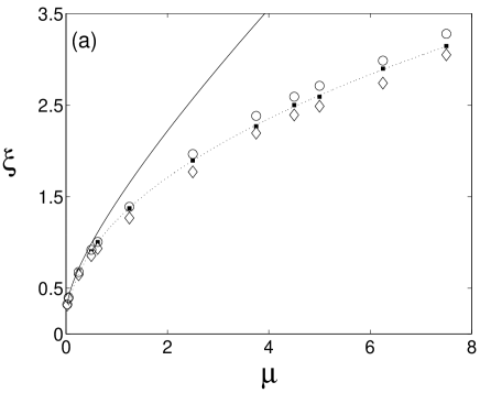
Figure 6: Characteristic cluster length $\xi$ given by the fits to data in Fig. 5. (a): Results of simulation (solid squares), the numerical RG of Sec. II (open circles) and an enhanced numerical RG with strain check (diamonds) described in Sec. IV.2. The solid line is a simple analytic prediction $\xi(\mu)=-1/\log(1-\wp(\mu))$ where $\wp(\mu)$ is defined in Eq. (31). The dashed line is a power law fit to the solid squares for $\mu>0.625$ and has an exponent of $0.46$; similar fits to the diamonds and circles give exponents of $0.48$ and $0.48$ respectively. (b): Log-log plot of the same data excluding the analytic prediction.

We find good agreement between the RG procedure (open circles) and simulation (solid squares) until $\mu\approx 5$, after which the two results begin to deviate from each other. The small, but growing discrepancy beyond $\mu=5$ suggests there is an additional mechanism in the physics of cluster formation that becomes important at larger $\mu$ and is not taken into account by the decimation steps of the RG procedure.

A physical effect that may not be adequately included in our RG procedure is the accumulation of phase strain as a cluster is built up through successive strong coupling decimation steps. We can understand this effect based on the arguments of Ref. Strogatz and Mirollo 1 . If we neglect the interactions of a synchronized cluster with the rest of the chain, its frequency is the average frequency $\langle\omega\rangle$ of the constituent oscillators. Furthermore, forming the sum of Eqs. (3) from one end of the cluster (here labeled 1) to the $n$th oscillator in the cluster gives

$$X_{n}=\sum_{i=1}^{n}(\omega_{i}-\langle\omega\rangle)=K_{n}\sin(\theta_{n+1}-\theta_{n}),$$ (29)

since the internal interaction terms cancel. We refer to this condition for the cluster’s existence as a strain check. The condition reads: $\left|X_{n}\right|<K_{n}$ for all $n$ in the cluster. Note that $X_{n}$ is the sum of random numbers, so that as the size of the cluster increases, the range of values of $|X_{n}|$ typically grows, and increasing phase strains $|\theta_{n+1}-\theta_{n}|$ are needed to keep the various parts of the cluster synchronized. If the strain becomes so large that some $|\theta_{n+1}-\theta_{n}|$ become $\pi/2$, the cluster will break. Also note that if two clusters are combined through a strong coupling decimation step to form a putative larger cluster, the mean frequency $\langle\omega\rangle$ to be used in the sum of Eq. (29) changes, and the condition $\left|X_{n}\right|<K_{n}$ may be violated for a bond in the interior of the two subclusters. This means that the combined set of oscillators are not in fact synchronized, and should be broken into smaller synchronized clusters in the RG procedure. We proceed by making the assumption that the oscillators form just two synchronized clusters, and identify the break between the two clusters as where the condition $\left|X_{n}\right|<K_{n}$ is violated in the presumed cluster. Thus if $X_{n}$ exceeds $K_{n}$ at some $n$, we do not allow the cluster to form. Instead, we re-form the bare oscillators into two different sub-clusters, such that the first sub-cluster is formed out of the bare oscillators $1$ through $n$ and the second is formed form the remaining bare oscillators. The RG then proceeds as normal. The new sub-clusters may be subjected to either of the two decimation steps later in the sweep, or in the next sweep if more are required.

The $\xi(\mu)$ obtained with the version of the RG which included the strain check are shown by diamonds in Fig. 6. The change in the results takes place in the right direction (decreasing $\xi$), but with a systematic over-estimation. All three sets of data, when plotted on a log-log scale follow approximately straight lines for $\mu>0.5$, so $\xi(\mu)$ appears to become a power law in this range. The straight-line fits to the data were made for $\mu>0.625$. The dashed curve in Fig. 6 is the fit to the simulation results, suggesting the behavior $\xi\propto\mu^{0.46}$ while the fits to the RG data with and without the strain check give $\xi\propto\mu^{0.48}$ and $\mu^{0.48}$.

IV.3 Estimate of $\xi(\mu)$

Given the simplicity of the renormalization group approach, one may wonder whether we can capture the behavior of the oscillator chain with a simple one-loop argument, based on the role of weak couplings in the limitation of cluster sizes.

Indeed, the small clusters are likely to form between weak couplings, and since the distribution of separations between such weak couplings follows Poisson statistics, an exponential distribution arises naturally. Using this hypothesis the probability of finding a cluster of size $n$ (i.e., a cluster delimited by two weak couplings $n$ units apart) is $P(n,\wp)=C(1-\wp)^{n}=Ce^{-n/\xi}$ where $\xi=-1/\ln{(1-\wp)}$ and $\wp$ is a probability that any randomly chosen coupling is weak. We make an estimate of this $\wp$ based on bare distributions of $\omega$ and $K$. Similarly to the RG, we define a coupling to be weak if $2K<\left|\omega_{l}-\omega_{r}\right|$. For each such bond, the probability that the required ratio is $>1$ is given by

$$\wp=2\int_{0}^{\infty}\left(\int_{-\infty}^{\infty}g(\omega)g(\omega+\delta)\,d\omega\right)\times\left(\int_{0}^{\delta/2}G(K)\,dK\right)\,d\delta$$ (30)

The integral of $g(\omega)g(\omega+\delta)$ is the probability that for each of the two oscillators connected by this bond, $\omega_{l}-\omega_{r}=\delta$. For each such frequency difference, all the bonds with $K<|\delta|/2$ are considered weak. Finally, all possible values of $\delta$ are integrated in the outer integral. After performing the inner integrals over $\omega$ and $K$ we obtain

$$\wp(\mu)=\frac{4}{\pi^{3}}\int_{0}^{\infty}\frac{2\pi}{4+\delta^{2}}\arctan{\left(\frac{\delta}{2\mu}\right)}\,d\delta.$$ (31)

This result is compared with both the RG predictions and numerical solutions in Fig. 6. The expression gives a good description of the data for $\mu\rightarrow 0$, but overestimates the characteristic cluster size for larger values of $\mu$. The renormalization group method, which does not treat all scales of frequencies and couplings at once, clearly provides better predictions then an estimation based on bare distributions.

V Conclusions

In this paper we investigated the collective behavior of a one-dimensional chain of coupled non-linear oscillators with random frequencies and nearest-neighbor couplings. For this purpose we developed a real space renormalization group approach, which is expected to be reliable in analyzing chains with large disorder. As we report above, our RG approach did an excellent job in capturing both the dynamics of individual oscillators, and the large scale behavior of the chain.

The disordered oscillator chain has the potential of establishing macroscopic order, which is exhibited by a finite fraction of all oscillators in the system moving in accord with the same frequency. Indeed in systems with higher connectivities, such global synchronization may occur, but in the limit of short ranged interactions, the macroscopic order is stymied by fluctuations. This dynamical behavior is reminiscent of critical phenomena in equilibrium statistical mechanics, where for each system there exists a lower critical dimension, and only dimensionality higher than that allows macroscopic ordering. In our analysis, we concentrated on the quantities that most directly capture the collective aspects of the chain’s behavior, and therefore also the competition between the interactions which seek to establish a synchronized phase, and the disorder-induced fluctuations which destroy it. This physics is fully contained in the cluster-size distribution, $P(n)\sim e^{-n/\xi(\mu)}$, which we find as a function of the interaction-strength tuning parameter, $\mu$.

The behavior of the average cluster size, $\xi(\mu)$, acts as an effective correlation length for the oscillator chain, where we once more think of our system in terms of the theory of critical phenomena. Since our oscillator chain is below its lower critical dimension, it’s phase diagram resembles that of the one-dimensional Ising model, with $\mu$ serving the role of inverse temperature $1/T$. The chain has an ordered phase, where all oscillators are synchronized, which is reached in the limit $\mu\to\infty$ (analogous to the Ferromagnetic phase at $T\to 0$). This phase, however, is described by an unstable fixed point. If an RG flow can be extended to the entire parameter space, the full-synchronization fixed point flows under RG to the stable fixed point found at the non-interacting point, $\mu=0$, which describes the unsynchronized phase (analogous to the paramagnetic fixed point at $T\to\infty$). The putative flow diagram of the chain is shown in Fig. 7. The flow from the fully-synchronized point to the unsynchronized $\mu=0$ point is indeed associated with a length scale, whose meaning is the coarse-graining length at which the chain seems fully unsynchronized, i.e., consisting of single free oscillators. This length is the size of synchronized clusters in the original chain, $\xi(\mu)$.

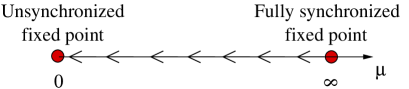
Figure 7: Fixed points and flow diagram of the oscillator chain. The short-range oscillator chain has only two fixed points: the unstable fully synchronized fixed point at infinite interactions (or zero disorder) $\mu\to\infty$, and the stable unsynchronized fixed point. The cross over flow between the two points is associated with a correlation length, captured by the average cluster size, $\xi(\mu)$.

Since $\xi(\mu)$ serves as an effective correlation length, it may diverge in a universal fashion in the limit $\mu\to\infty$. While our RG method can only access moderate values of $\mu$, we cautiously argue that we can access the critical region, as can be seen in Fig. 5. From our results we obtain the critical exponent $\nu$ of the synchronization transition:

$$\xi(\mu)\sim\mu^{\nu}\hskip 28.45274pt\nu\simeq 0.48$$ (32)

Note that this behavior is not analogous to the divergence of the Ising chain correlation length $\xi\sim\ln\frac{1}{T}$.

The method by which we obtained the above results constitutes the main achievement of this work. We developed a real space renormalization group scheme that successfully predicts the detailed behavior of a nonlinear oscillator chain with short-range interactions. We have implemented the RG scheme numerically on a chain of $10^{6}$ oscillators and compared its results with essentially exact simulations of the model equations, Eqs. (3) (see Sec. III). The agreement is very good, and for some characteristics, such as the cluster frequency distributions at low frequencies, it improves with larger cluster sizes. This indicates particularly that our local RG scheme successfully captures the non-trivial collective features of the chain expressed in large synchronized clusters.

One practical implication of our analysis may be found when considering coupled laser arrays, where only limited connectivity can be achieved. Diode lasers, for example, are manufactured in one-dimensional bars that allow for evanescent coupling through overlapping electric fields. Due to the exponential fall-off in the electric field envelope with distance, the coupling between well-behaved diodes can only be short ranged. The tools developed here could be used to study the extent of coherence that such systems exhibit. A potentially promising area of current research is constructing grids of diodes coupled in 2-dimensions by stacking 1-dimensional bars. Our RG technique could possibly also be extended to such a system, and help clarify both its properties, and whether it can establish macroscopic coherence.

Our work suggests several other directions for future research. First, we may ask how can one improve the applicability of our RG scheme to larger values of the interaction parameter $\mu$. This may be pursued by focusing on the concept of intra-cluster strain, which is roughly the variance of phase differences between neighboring oscillators within a cluster. As interaction increases, cluster sizes grow, and bigger strain is needed to accommodate the spread of frequencies within a cluster (cf. Sec. IV.2). In our current scheme we made the first attempt to take this into account with the strain check based on the argument of Strogatz and Mirollo 1 , a condition expressed by Eq. (29). This led to some improvement - for example, $\xi(\mu)$ was modified in the right direction, but this modification was over-estimated. The strain check may be augmented in the future.

A second natural question is the degree of universality in the oscillator chain. Our result for the correlation length critical exponent $\nu$, Eq. (32), was obtained using Lorentzian distributions. It is possible that the exponent depends on the nature of the tails of the distributions used; Lorentzians, for instance, do not have a variance. We intend to investigate the universality of $\nu$ alongside investigating the applicability of our RG scheme to distributions with narrower tails.

A more general question concerns the development of an RG scheme and the analysis of synchronization in short-range networks at higher dimensions, and especially at two dimensions, which is very close to the lower critical dimension: Refs. Anamalous ; Daido suggest that in two dimensions there may be a transition to a macroscopically synchronized phase, or that $d=2$ is the lower critical dimension giving rise to interesting anomalous behavior (see also Acerbon's_review ). The development of a decimation procedure at dimensions higher than one is quite challenging because of the higher connectivity of the system, and the possibility that real-space local decimation steps change the geometry of the system.

It is a pleasure to thank Heywood Tam for numerous discussions and Tony Lee for carefully checking the RG procedure. We are also grateful to Boeing and the National Science Foundation under Grant No. DMR-0314069 for funding this work.

References

- (1) A. Pikovsky, Synchronization: A Universal Concept in Nonlinear Science, Cambridge University Press, New York, 2001.
- (2) F. Varela, J. P. Lachaux, E. Rodriguez, J. Martinerie, Nature Reviews Neurosci. 2, 229 (2001).
- (3) A. K. Engel and W. Singer, Trends Cognit. Sci. 5, 16 (2001).
- (4) M. Rabinovich, P. Varona, A. Selverston, H. Abarbanel, Rev. Mod. Phys. 78, 1213 (2006).
- (5) K. Wiesenfeld, Physica B 222, 315 (1996).
- (6) B. R. Trees, V. Saranathan, and D. Stroud, Phys. Rev. E 71, 016215 (2005).
- (7) B. R. Trees, S. Natu, and D. Stroud, Phys. Rev. B 72, 214524 (2005).
- (8) A. G. Vladimirov, G. Kozyreff, and P. Mandel, Europhys. Lett. 61, 613 (2003).
- (9) J. F. Heagy, T. L. Carroll, and L. M. Pecora, Phys. Rev. E 50, 1874 (1994)
- (10) S.K. Esser, S.L. Hill, G. Tononi, Sleep, 30, 1617 (2007).
- (11) J.J. Collins, I.N. Stewart, J. Nonlinear Sci., 3, 349 (1993).
- (12) L. Glass, Nature, 410, 277 (2001).
- (13) J. A. Acerbon, et. al., Rev. Mod. Phys., 77, 137 (2005).
- (14) Y. Kuramoto, in: H. Araki (Ed.), International Symposium on Mathematical Problems in Theoretical Physics, lecture Notes in Physics. Vol. 39, Springer, New York, p. 420, 1975.
- (15) Y. Kuramoto, Chemical Oscillations, Waves, and Turbulence, Springer, Berlin, 1984.
- (16) B. C. Daniels, S. T. M. Dissanayake, and B. R. Trees, Phys. Rev. E 67, 026216 (2003).
- (17) F. Rogister and R. Roy, Phys. Rev. Lett. 98, 104101 (2007).
- (18) S. H. Strogatz, R. E. Mirollo, J. Phys. A: Math. Gen. 21, L699-L705 (1988).
- (19) S.H. Strogatz, R. E. Mirollo, Physica D 31, 143-168 (1988).
- (20) S. K. Ma, C. Dasgupta and C. K. Hu, Phys. Rev. Lett., 43, 1434 (1979).
- (21) C. Dasgupta and S. K. Ma, Phys. Rev. B, 22, 1305 (1980).
- (22) D. S. Fisher, Phys. Rev. B, 50, 3799 (1994).
- (23) D. S. Fisher, A. P. Young, Phys. Rev. B, 58, 9131 (1998).
- (24) E. Altman, Y. Kafri, A. Polkovnikov, G. Refael, Phys. Rev. Lett. 93, 150402 (2004)
- (25) E. Altman, Y. Kafri, A. Polkovnikov, G. Refael, Phys. Rev. Lett. 100, 170402 (2008).
- (26) Oleg Kogan, ”Stochastic and collective properties of nonlinear oscillators” (Ph.D. thesis, California Institiute of Technology, 2008), to be submitted.
- (27) H. Sakaguchi, S. Shinomoto, and Y. Kuramoto, Prog. Theor. Phys. 77, 1005 (1987).
- (28) H. Daido, Phy. Rev. Lett. 61, 231 (1988).