Quantum Nucleation and Macroscopic Quantum Tunneling in Cold-Atom Boson-Fermion Mixtures

Abstract

Kinetics of phase separation transition in boson-fermion cold atom mixtures is investigated. We identify the parameters at which the transition is governed by quantum nucleation mechanism, responsible for the formation of critical nuclei of a stable phase. We demonstrate that for low fermion-boson mass ratio the density dependence of quantum nucleation transition rate is experimentally observable. The crossover to macroscopic quantum tunneling regime is analyzed. Based on a microscopic description of interacting cold atom boson-fermion mixtures we derive an effective action for the critical droplet and obtain an asymptotic expression for the nucleation rate in the vicinity of the phase transition and near the spinodal instability of the mixed phase. We show that dissipation due to excitations in fermion subsystem play a dominant role close to the transition point.

I Introduction

Macroscopic metastable states of trapped cold atom systems have been a subject of active experimental and theoretical study for more than a decade UedaLeggett . Unlike a homogeneous system of bosons, where infinitesimally small attractive interaction between atoms leads to a collapse, trapped bosons are known to form long lived Bose-Einstein Condensates UedaLeggett ; Modugno (BEC) due to zero-point energy which, for sufficiently low densities, can compensate the negative interaction energy thus maintaining the system in equilibrium. Upon increasing the BEC density, interaction energy grows, and, at some instability point (i.e., at a certain number of particles in the trap $N_{c}$, with $N_{c}\sim 10^{3}$ for a typical trap), zero-point energy can no longer sustain the negative pressure due to the interactions and the system collapses. It has been argued in the literature UedaLeggett that near the instability point (for BEC densities slightly lower than the instability density), the effective energy barrier that prevents BEC from collapsing becomes so low that the system can quantum mechanically tunnel into the dense (collapsed) state.

Such phenomenon of Macroscopic Quantum Tunneling (MQT), however, has never been observed experimentally due to a strong dependence of the barrier height on the total number of particles in the trap ($N$). Indeed it has been shown UedaLeggett that the tunneling exponent for such a transition near the instability point scales as $N(1-N/N_{c})^{5/4}$ and therefore very fine tuning of the total particle number $N$ is required in order to keep the tunneling exponent relatively small [$(1-N/N_{c})\ll 1$]. Since for most BEC setups the total number of the trapped atoms fluctuates and typically obeys Poissonian statistics, the error in $N$ scales as $N^{1/2}$ and therefore such a stringent requirement is hard to fulfill. Thus the system is typically either in a sub-critical state with no barrier present ($N\geq N_{c}$) or is in the state with very high energy barrier and therefore very low MQT rate.

In this paper we propose another paradigm for observation of tunneling driven phase transition effects in cold atom systems based on the theory of quantum nucleation LifshitzKagan ; LifshitzKhokhlov ; Burmistrov . It has long been known that a mixture of ³He-⁴He undergoes a phase separation transition at relative concentration of ³He in ⁴He of around $6\%$ at temperatures close to the absolute zero Edwards . Since such a phase separation is a first order phase transition (it is observed to be accompanied by the latent heat release down to mK temperatures), the order parameter must have some finite (microscopic) correlation length and therefore the transition is expected to occur through the formation of nuclei of the new stable phase in the old metastable one. As usual, dynamics of the nucleation process is controlled by the competition of the surface and bulk energies of the nuclei and therefore, in order for a given nucleus to become stable (supercritical), it must overcome a potential barrier formed by the two above contributions. While in most systems such a transition is a thermally activated process, it has been argued that in the ³He-⁴He mixture at sufficiently low temperatures (below 100 mK) the transition is driven by the quantum tunneling. In particular, it was predicted LifshitzKagan ; Burmistrov that near the transition line the tunneling exponent for such a transition rate is proportional to $\Delta\mu^{-7/2}$, where $\Delta\mu$ is the difference in the chemical potentials of the two phases. It has later been found experimentally HeExperiment that below 80 mK kinetics of such phase separation transition becomes independent on temperature and therefore it must be driven by the quantum tunneling. However, the experiments have been unable to verify the expected dependence of the nucleation rate on the systems’s parameters (i.e., $\Delta\mu$, etc) - partly due to the poor knowledge of microscopic interactions between particles in such a strongly correlated system.

We argue that contemporary cold atom systems provide an excellent candidate for studying and observing the kinetics of such a phase separation transition in boson-fermion mixtures SELF . Mixtures of boson and fermion atoms are typically realized in experiments studying fermionic superfluidity, where bosons play role of a coolant BosCool . Another interesting realization of boson-fermion mixture has been demonstrated in two-component fermion system, where strongly bound Cooper pairs correspond to bosons interacting with unpaired fermion atoms Ketterle . In the present paper we begin with detailed derivation and analysis of the results outlined in Ref. SELF, . Significant attention is given to supercritical dynamics, which reflects the dissipative mechanisms and is measurable in less interacting system.

Starting from a microscopic description of a boson-fermion mixture we derive an effective action for the order parameter (the BEC density) taking into account fermion-boson interaction. We show explicitly that the classical potential for the order parameter due to such interaction has two minima corresponding to the two phases of the system (mixed and phase separated), see Sec. III. We analyze the coherence length associated with the system and demonstrate that it varies from finite to divergent and therefore allows different mechanisms for the phase transition, see Sec. IV. At low fermion densities the two minima of the potential are separated by the finite energy barrier resulting in finite coherence length, which points out that such a transition is of the first order bosons ; Timmermans . We then derive an expression for the nucleation (tunneling) rate of the critical droplet of the pure fermion phase near the phase transition line and near the line of absolute (spinodal) instability of the mixed phase in Secs. VI and VII. We show that the transition rate is measurable (of the order $0.1-1$s${}^{-1}\mu$m^-3) for densities reasonably close to the phase transition line and small fermion-boson mass ratio. The limitation on the mass ratio comes as the result of dissipative dynamics due excitations in fermion system. Near the phase transition line it leads to significant modification (increase) of the transition rate for the system with high fermion-boson mass ratio, in which case the observable transition rates exist closer to the line of absolute instability (where the dissipation is less effective and the tunneling exponent becomes reasonably small). Our results for this regime are similar to those obtained in Ref. UedaLeggett, for the MQT in the systems of trapped bosons with attractive interactions. However, in the case of boson-fermion separation transition the height of the potential barrier and, thus, the tunneling exponent are controlled not by the total number of particles in the trap, but their densities, scaling as $(1-n/n_{c})^{1/2}$. Therefore, for sufficiently large numbers of particles in the trap the tunneling exponent can be fine-tuned with a desired accuracy which makes it possible to observe the MQT rate in a well controlled and predictable regime.

II Model

We consider a Bose-Einstein Condensate (BEC) interacting with a single species of fermions (in the same spin state). Interactions in such the mixture are characterized by two scattering lengths $a_{BB}$ and $a_{BF}$. Fermions and bosons interact through contact potential $\lambda_{BF}\delta(\mathbf{r}-\mathbf{r}^{\prime})$, contributing term $\lambda_{BF}\psi_{B}^{\dagger}\psi_{F}^{\dagger}\psi_{B}\psi_{F}$, where $\lambda_{BF}=2\pi\hbar^{2}a_{BF}(1/m_{B}+1/m_{F})$; $\psi_{B}$ and $\psi_{F}$ are boson and fermion fields respectively. In addition, boson-boson particle interaction give rise to another term $\lambda_{BB}\psi_{B}^{\dagger}\psi_{B}^{\dagger}\psi_{B}\psi_{B}/2$ in the Hamiltonian density, with $\lambda_{BB}=4\pi\hbar^{2}a_{BB}/m_{B}$. The direct coupling between fermions is negligible: s-scattering channel is forbidden for the fermions in the same spin state, while p-wave scattering is small compared to boson-boson and boson-fermion contact interaction. The potential part of the energy density can be cast in the form

$$E_{p}= - \mu_{B}|\psi_{B}|^{2}-\mu_{F}\psi_{F}^{\dagger}\psi_{F}$$

$$+ \frac{\lambda_{BB}}{2}|\psi_{B}|^{4}+\lambda_{BF}|\psi_{B}|^{2}\psi_{F}^{\dagger}\psi_{F}$$

For the purposes of the present calculation we can neglect the spatial dependence of the trapping potential and assume that the local densities of fermions and bosons are set by the constant chemical potentials $\mu_{F}$ and $\mu_{B}$. Indeed, since the nucleation occurs at finite coherence length (to be defined below), the shape of the trapping potential should play little role in the dynamics of the phase transition as long as the effective size of the trap is much greater than the coherence length.

It is convenient to describe the system in terms of the boson field only, tracing $e^{-H/k_{B}T}$ ($H$ is the overall Hamiltonian) with respect to the fermion field. Such averaging can be easily carried out within mean field, i.e., the Thomas-Fermi approximation Mahan ; Viverit ; Mozyrsky , so that the calculation reduces to the evaluation of the canonical partition function (or free energy) of the free fermions with effective chemical potential $\tilde{\mu}_{F}=\mu_{F}-\lambda_{BF}|\psi_{B}|^{2}$. Later, in Sec. IV, we will proceed beyond this approximation and account for the fermion excitations interacting with the condensate. For the purpose of this and the following section such a correction is not necessary.

Within Thomas-Fermi approximation Mahan we deal with the energy density of free fermions in the zero-temperature limit. It can be easily found differentiating fermion free energy $\sqrt{2}Vm_{F}^{3/2}\tilde{\mu}_{F}^{5/2}/{5\pi^{2}\hbar^{3}}$ with respect to the volume (note that $\tilde{\mu}_{F}\sim V^{-2/3}$). We finally obtain the effective classical potential density for the bosons

$$E(\rho)= - \mu_{B}\rho+\frac{1}{2}\lambda_{BB}\rho^{2}$$

$$- \lambda_{0}\left(\mu_{F}-\lambda_{BF}\rho\right)^{5/2}\theta(\mu_{F}-\lambda_{BF}\rho),$$

where $\theta(x\geq 0)=1$, $\theta(x<0)=0$, $\lambda_{0}=(2m_{F})^{3/2}/15\pi^{2}\hbar^{3}$, and we have used the density–phase variables, i.e. $\psi_{B}=\sqrt{\rho}e^{i\phi}$, for the condensate field. The approximation discussed above ignores gradient terms in the diagrammatic expansion of the partition function Kleinert ; ImambekovDemler . This terms are not important for the phase structure of the equilibrium system and will be discussed in Sec. IV.

In the next section we discuss the structure of the phase diagram describing possible configurations in the equilibrium boson-fermion system. Subsequent sections are devoted to the kinetics of the transition. The transition rates are calculated in Secs. VI and VII. Sections VIII and IX are devoted to the discussion of thermal activation and supercritical expansion. The results are discussed in Sec. X.

III System in Equilibrium: The Phase Diagram

Equation (II) was obtained tracing over the fermionic part of the partition function. In this respect, it can be viewed as effective potential energy of boson condensate. The structure of the fast fermionic part of the system, in particular the density of fermions, is directly related to the state of the boson condensate. In the limit of zero temperatures we obtain the fermion density in the form

$$\rho_{F}(\rho)=\frac{5}{2}\lambda_{0}(\mu_{F}-\lambda_{BF}\rho)^{3/2}\theta(\mu_{F}-\lambda_{BF}\rho)$$ (3.1)

where the chemical potential $\mu_{F}$ is the same for all parts of the system in the mixture as far as the time scale of slow boson subsystem is of interest.

It was shown within Thomas-Fermi approximation Viverit that the equilibrium boson-fermion system with interactions introduced above can exist in three configurations (phases): (i) mixture, (ii) coexistence of pure fermion fraction with (spatially separated) mixture, and (iii) coexistence of pure boson and pure fermion fractions, see Fig. 1. In this section we show that the structure of the entire phase diagram can be obtained from the energy density (II). Indeed, we notice that $E(\rho)$ has either one or two local minima. The first one (if present) is at $\rho=0$. It clearly describes pure fermion fraction with the density of fermion $\rho_{F}(0)$. The position of the second minimum is found from $\partial_{\rho}E(\rho_{0})=0$. It describes either the mixture with fermion density $\rho_{F}(\rho_{0})>0$, or the pure boson fraction with $\rho_{F}(\rho_{0})=0$ due to the step function in Eq. (3.1).

We first discuss the situation when the thickness of the transition region (boundary) between the fractions, or the coherence length, $l$, is microscopic (i.e. small with respect to the characteristic size of the fractions). In this case it is natural to introduce the overall (average) fermion $\rho_{F}=\rho_{F}(0)V_{F}+\rho_{F}(\rho)V_{B}$ and boson $\rho_{B}=V_{B}\rho$ densities of a larger system. Here $V_{F}$ and $V_{B}=1-V_{F}$ are relative volumes for each fraction.

When the densities $\rho_{B}$ and $\rho_{F}$ are small, the minimum at $\rho=\rho_{0}$ is the only one present. At low temperatures the equilibrium system will occupy this minimum creating uniform mixture (phase i) with $\rho_{F}=\rho_{F}(\rho_{0})$ and $\rho_{B}=\rho_{0}$ ($v_{F}=0$). At higher densities the minimum at $\rho=0$—the pure fermion fraction—forms. As a result, in equilibrium, the two minima align, $E(0)=E(\rho_{0})$, which defines the volume of the spatially separated fermion fraction.

For clarity of further discussion it is convenient to introduce dimensionless densities Viverit as

$$n_{F}\equiv\rho_{F}a_{BB}^{3}/g_{1}^{2}\quad\mathrm{and}\quad n_{B}\equiv\rho_{(B)}a_{BB}^{3}/g_{0}^{2}.$$ (3.2)

Here and throughout the paper we adopt the convention of using “n” for dimensionless densities corresponding to original densities denoted by “$\rho$”. The conversion parameters of Eq. (3.2) are

$$g_{0}^{2}=\frac{4a_{BB}^{3}\lambda_{BB}^{2}}{25\lambda_{0}^{2}\lambda_{BF}^{5}}=\frac{9\pi}{4}\frac{a_{BB}^{5}}{a_{BF}^{5}}\frac{m_{F}^{2}}{m_{B}^{2}}\left(\frac{m_{F}}{m_{B}}+1\right)^{-5}$$ (3.3)

and

$$g_{1}^{2}=\frac{4a_{BB}^{3}\lambda_{BB}^{3}}{25\lambda_{0}^{2}\lambda_{BF}^{6}}=\frac{9\pi}{2}\frac{a_{BB}^{6}}{a_{BF}^{6}}\frac{m_{F}^{3}}{m_{B}^{3}}\left(\frac{m_{F}}{m_{B}}+1\right)^{-6}$$ (3.4)

where $g_{0}$ is related to boson gas parameter (defined LifshitzPitaevskii via $g_{B}=\sqrt{\rho_{B}a_{BB}^{3}}$) as $g_{B}^{2}=g_{0}^{2}n_{B}$.

The separation between phases i and ii on the phase diagram ($n_{F}$ vs $n_{B}$) occurs when $V_{F}$ sets to zero. The corresponding phase separation curve can be easily obtained in a parametric form as follows. Introducing $A\equiv\lambda_{BB}/5\lambda_{0}\lambda_{BF}^{2}\mu_{F}^{1/2}$ and $y^{2}\equiv 1-\rho_{0}\lambda_{BF}/\mu_{F}$ one can write the boson and fermion densities in the mixture fraction as

$$n_{F}^{0}=\frac{y^{3}}{8A^{3}}\quad\mathrm{and}\quad n_{B}^{0}=\frac{1-y^{2}}{4A^{2}}.$$ (3.5)

The equilibrium mixture coexists with unoccupied ($V_{F}\to 0$) pure fermion minima only at the i-ii phase transition curve. In terms of $A$ and $y$, the equation $E(0)=E(\rho_{0})$ takes the form

$$A=\frac{2+4y+6y^{2}+3y^{3}}{5(1+y)^{2}}$$ (3.6)

which, together with Eq. (3.5) defines the phase transition curve: $n_{F}^{0}$ vs $n_{B}^{0}$. From Eq. (3.6) we also see that $A$ varies within $2/5\leq A\leq 3/4$ (since by definition $0\leq y\leq 1$ within phase ii).

The complete separation on pure fermion and pure boson fractions (phase iii) occurs for higher densities when $\rho_{0}\geq\mu_{F}/\lambda_{BF}$. This situation is not considered in the present paper.

In the discussion above, it was assumed that in the phase ii the fermion fraction is spatially separated from the mixture and the volume of the surface layer is negligible. This is not always the case as will be demonstrated in the next section. However when $l$ is large, one can still define effective partial volumes $V_{F}$ and $V_{B}$, assuming that the densities discussed above are the peak densities. While the relation between $V_{F}$ and $V_{B}$ is now complicated, the limit $V_{F}\to 0$ with $V_{B}\to 1$ still exists. Therefore, the i-ii separation curve found above is valid.

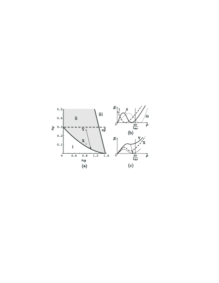
Figure 1: The phase diagram of the uniform boson-fermion mixtures. Three phase are possible: (i) mixture, (ii) coexistence of pure fermions with mixed fraction, (iii) coexistence of pure fermion and pure boson fractions. The arrow indicates the path of the mixture fraction as the system equilibrates. The instability level is represented by the dashed horizontal line on the phase diagram. The densities are in units of $g_{0}^{2}/a_{BB}^{3}$ and $g_{1}^{2}/a_{BB}^{3}$ for bosons and fermions respectively, as defined in Eq. (3.2). The inset (b) shows the sketch of $E(\rho)$ at equilibrium for the corresponding phases. The inset (c) gives the sketch of $E(\rho)$ near (below) the instability line and (above) the phase separation curve. The arrow indicates (schematically) modification of $E(\rho)$ during the equilibration.

IV Dynamics of Quantum Transition

We are interested in the kinetics of the phase transition between phases i and ii, which is manifested by separation of pure fermion fraction out of the mixture. When the uniform mixture is prepared with the densities $n_{F}$ and $n_{B}$ above the i-ii separation curve, e.g. point X, it occupies the second minima of $E(\rho)$ and is metastable, see Fig. 1c. As $n_{F}$ increases towards the point Y (and further) the barrier that separates local minima $\rho_{0}$ becomes smaller and eventually disappears from $n_{F}\geq n_{F}^{s}$, with $n_{F}^{s}=8/27$ (the absolute, spinodal, instability line). From this point the mixture becomes unstable.

The decay of the metastable mixture results in spatial separation of pure fermion fraction. At low temperatures this transition is governed by quantum tunneling (in contrast to high temperatures, when thermal activation becomes effective and transition is due to thermal fluctuations rather then tunneling). To illustrate the equilibration process, let us assume that the coherence length, $l$, is small enough so that the spatial separation of the fermion fraction is well defined. Towards the end of this section we will show where such condition is met. During the equilibration, the relative volume $V_{F}$ of the fermion fraction increases from 0 to some equilibrium value $V_{F}^{0}$. The densities $\rho_{0}$ and $\rho_{F}(\rho_{0})$ of the remaining mixture will change, as well as $E(\rho)$. The point $(\rho_{0},\rho_{F}(\rho_{0}))$ will drift towards i-ii separation curve where $E(0)=E(\rho_{0})$, as shown by the arrow in Figs. 1a and 1c. As it can be easily verified, the drift line is parallel to ii-iii separation line and its intersection with the $n_{F}$ axis gives the equilibrium value for the density in pure fermion fraction, $\rho_{F}(0)$. The partial volume of the later is $V_{F}^{0}=(n_{B}^{0}-n_{B})/n_{B}^{0}$.

In what follows we will obtain the density profile for the fermion droplet in various regions of the phase diagram (within phase ii) and set up equations to describe the transition rate in the system. The rates are calculated in the next sections.

The dynamics of the boson condensate due to tunneling part of the equilibration is given by the transition amplitude ${\langle ii^{\prime}|}e^{-iHt}{|i^{\prime}\rangle}=\int\mathcal{D}\psi_{B}\mathcal{D}\psi_{B}^{*}e^{i\int dtd\mathbf{r}L(\psi_{B},\psi_{B}^{*})}$, where the rhs is Feynman’s sum over the histories Kleinert ; Coleman . The state ${|i^{\prime}\rangle}$ represent the (non-equilibrium) metastable mixture residing in the second minimum of $E(\rho)$, at $\rho\to\rho_{0}$. The state ${|ii^{\prime}\rangle}$ correspond to the state after the tunneling with $\rho\to\rho_{1}$, $E(\rho_{1})=E(\rho_{0})$. Beyond this point the system hydrodynamically equilibrates to the state ${|ii\rangle}$ where the two minima get aligned, see Fig 1b, curve ii. The Lagrangian density is defined as $L(\psi_{B},\psi_{B}^{*})=\psi_{B}^{*}i\hbar\partial_{t}\psi_{B}-H(\psi_{B},\psi_{B}^{*})$, where the Hamiltonian density contains the kinetic $\hbar^{2}|\nabla\psi_{B}|^{2}/2m_{B}$ and potential $E(\rho)$ contributions, where the latter is considered within the Thomas-Fermi approximation, see Eq. (II).

As it has been pointed out earlier, approximation for $E(\rho)$, i.e. Eq. (II), does not account for the gradient terms which arise due to inhomogeneity of the fermion subsystem and add to $\hbar^{2}|\nabla\psi_{B}|^{2}/2m_{B}$ term of the Lagrangian density. In other words, the approximation implies that renormalization of the boson kinetic energy arising due to the non-locality of the fermionic response function is relatively small. A straightforward perturbative estimate Kleinert to the second order in $\lambda_{BF}$ yields the gradient term correction to the Thomas-Fermi of the order $\sim(m_{F}^{3/2}\!\lambda_{BF}^{2}\mu_{F}^{1/2}/\hbar^{3}k_{F}^{2})(\nabla\rho)^{2}$. Comparing this term with the bare boson kinetic energy, we see that near the phase transition line it is smaller by the factor of $\sim(m_{B}\!/m_{F})^{2/5}g_{B}^{2/5}n_{B}^{4/5}\!\!/n_{F}^{2/3}$. Therefore, for sufficiently low $g_{B}$ and not very small fermion densities the renormalization correction is negligible. This is clearly the case in the region near the spinodal instability line. In the vicinity of the phase separation line the renormalization correction can become important (e.g. closer to the tricritical point where $n_{F}\to 0$). In this case the correction is given by the factor of $\sim(k_{F}l)^{-2}$, where the coherence length $l$ is of the order $a_{BB}/g_{B}$ or greater (as will be demonstrated shortly). For $g_{B}\lesssim 0.1$ and not too small $n_{F}$ (e.g. for $n_{B}\sim 0.4$), $(k_{F}l)^{2}\sim 50$, and thus the Thomas-Fermi approximation is well justified.

Considering the above arguments, the transition can be described by the effective Lagrangian density of the form

$$L=\hbar\rho\frac{d}{dt}\phi+\frac{\hbar^{2}\rho}{2m_{B}}\left(\nabla\phi\right)^{2}+\frac{\hbar^{2}}{2m_{B}}\frac{\left(\nabla\rho\right)^{2}}{4\rho}+E(\rho).$$ (4.1)

Here the first term can be viewed as the Berry phase; the second and the third terms arise due to the kinetic energy; the dissipative terms due to particle-whole excitations in the fermion subsystem will be included later. The contribution due to non-condensate component of bosonic system is already accounted for by the above treatment and therefore separate consideration is not necessary for the purpose of the present calculation.

The decay rate from a metastable state can be obtained Coleman by calculating the classical action for the transition amplitude in imaginary time formalism, $it\to t$. Namely,

$$\Gamma/V=(\Gamma_{0}/V)\exp(-S/\hbar)$$ (4.2)

where the action $S=\int dtd\mathbf{r}L(\rho_{\textrm{cl}},\phi_{\textrm{cl}})$ is evaluated over the classical (extremal) trajectory, $\rho_{\textrm{cl}}(\phi_{\textrm{cl}})$. As will be shown below, for the parameters of interest, the rate is dominated by the exponent and is less sensitive to the changes in prefactor $\Gamma_{0}/V$. Therefore precise evaluation of $\Gamma_{0}/V$ is not crucial. It can be estimated as $\Gamma_{0}/V\sim\omega_{0}l^{3}$, where $l$ is boson coherence length as before, and $\omega_{0}$ is an “attempt” frequency. From the uncertainty principle $\omega_{0}\sim\hbar/2m_{B}l^{2}$ and thus $\Gamma_{0}/V\sim\hbar/m_{B}l^{5}$.

The extremal action $S$ is calculated by setting the corresponding functional derivatives to zero, i.e. $\delta L/\delta\rho=0$ and $\delta L/\delta\phi=0$. The second derivative is trivial. It leads to the continuity equation

$$\partial_{t}\rho+\nabla(\rho{\bf{u}})=0$$ (4.3)

with $\mathbf{u}=\hbar\nabla\phi/m_{B}$ and can be used to eliminate $\phi$. Equation. (4.3) can be easily solved for the velocity of the condensate assuming spherical symmetry. The result is $\mathbf{u}=({\mathbf{\hat{r}}}/{r^{2}\rho})\int_{0}^{r}dr{r^{2}\partial_{t}\rho}$. After a straightforward algebra the action becomes

$$S=4\pi\int dtdrr^{2}\left[\frac{m_{B}}{2\rho}\left(\frac{1}{r^{2}}\int_{0}^{r}drr^{2}\partial_{t}\rho\right)^{2}\right.$$ (4.4)

$$\left.+\frac{\hbar^{2}}{2m_{B}}\frac{\left(\nabla\rho\right)^{2}}{4\rho}+E(\rho)\right].$$

The pure fermion fraction to be formed during the equilibration corresponds to the bubble in the boson system. Its shape is defined by the last two terms of Eq. (4.4), i.e. the equation $\delta S/\delta\rho=0$ in the static case,

$$\partial_{r}^{2}\sqrt{\rho}+\frac{2}{r}\,\partial_{r}\sqrt{\rho}=\frac{m_{B}}{\hbar^{2}}\,\partial_{\sqrt{\rho}}E(\rho)$$ (4.5)

To solve it, let us first ignore the the second term of the left-hand side, which is a reasonable approximation for large enough bubbles. The solution of the remaining equation can be easily estimated for all relevant area of the pase diagram, see Appendix A. Near the i-ii separation curve we obtain

$$\rho(r)\sim\frac{\rho_{0}}{1+\exp[-4(r-R)/l_{0}]}$$ (4.6)

where the coherence length, $l\to l_{0}$ is

$$\frac{l_{0}}{a_{BB}}\sim\frac{1}{g_{0}n_{B}}$$ (4.7)

Near the spinodal instability the first-derrivative term becomes important. The density $\rho(r)$ varies between $\rho_{1}$ and $\rho_{0}$. The coherence length $l\to l_{s}$ is found, see Appendix A, in the form

$$\frac{l_{s}}{a_{BB}}=\frac{\sqrt{3}}{g_{0}\sqrt{\pi n_{B}}}\left(1-\frac{n_{F}}{n_{F}^{s}}\right)^{-1/2}+{\cal O}\left(1-\frac{n_{F}}{n_{F}^{s}}\right)$$ (4.8)

The estimate of $l$ for all the densities of phase ii below instability is given in Fig. 2a (see Appendix A for derivations). For not too small $g_{0}$ the characteristic length associated with the transition region is microscopic, i.e. $l\sim a_{BB}$. This is the case for large part of the interval $n_{F}^{0}\leq n_{F}<n_{F}^{s}$, see Fig. 2a. Therefore formation of a distinct fermion fraction with thin boundary (nucleation) is expected for this range of parameters. It is straightforward to obtain the characteristic (critical) radius, $R_{c}$ of such a nuclei. Integrating both sides of Eq. (4.5) with respect to $\sqrt{\rho}$ we obtain $m_{B}\Delta E/\hbar^{2}=2\int_{0}^{\rho_{0}}d\sqrt{\rho}\partial_{r}\sqrt{\rho}/r$. When $l\ll R$, we have $R_{c}=\sigma/\Delta E$, where $\sigma\equiv(2\hbar^{2}/m_{B})\int_{0}^{\rho_{0}}d\sqrt{\rho}\partial_{r}\sqrt{\rho}$ is the surface tension.

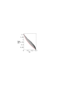
Figure 2: (a) The reciprocal coherence length as a function of dimensionless fermion density, $n_{F}$, for different values of dimensionless boson density of the mixture: $n_{B}=0.1,0.2,...,1.5$ (from bottom to top). The dashed curve represents reciprocal coherence length at the i-ii phase separation curve.

V Effect of dissipation

We now consider the effect of dissipation which was ignored so far in our description of the kinetics. Excitation of the particle-hole pairs in the fermion subsystem interacting with the condensate affects the transition, as it happens for other systems with quantum tunneling CaldeiraLeggett ; DSVB ; DMmosfet ; DSmosfet ; VBDS . As will be demonstrated further, the resulting dissipation is important and can lead to significant modifications of the transition rate.

The dissipation terms arise naturally from more accurate treatment of the boson-fermion interaction. Indeed, the Thomas-Fermi approximation utilized in the derivation of the effective potential $E(\rho)$, see Secs. II and IV, implies that fermions instantaneously (on a much shorter time scale) adjust to the local variation of boson density: it ignores the $\omega$-dependent terms in the diagrammatic expansion of the partition function. The effect can be analyzed by considering the second order correction produced by the interaction $\lambda_{BF}\psi_{F}^{\dagger}\psi_{F}\rho$.

$$\frac{{\lambda_{BF}^{2}}}{{2\hbar^{2}}}\int{\frac{{d{\bf{q}}}}{{\left({2\pi}\right)^{3}}}\frac{{d\omega}}{{2\pi}}\left({\frac{{\hbar^{2}k_{F}^{3}}}{{4\pi^{2}\mu_{F}}}+\frac{{m_{F}^{2}\left|\omega\right|}}{{4\pi\hbar^{2}q}}+...}\right)\left|{\rho(q,\omega)}\right|^{2}}.$$ (5.1)

The first $\omega$ independent term is already present in Eq. (II). We are after the frequency dependent term $m_{F}^{2}|\omega|/4\pi\hbar^{2}q$ responsible for Landau damping.

In the limit $l\ll R$, i.e. near the phase separation curve and far enough from the instability line, we can use $\rho(r)\approx\rho_{0}\theta(r-R)$ as suggested by Eq. (4.6). Substitution into Eq. (5.1) gives the correction to $S$ in the form

$$\Delta S\to\frac{\gamma_{0}}{64\pi}{\cal P}\int{dtdt^{\prime}\over(t-t^{\prime})^{2}}\left\{R(t)^{3}R(t^{\prime})\phantom{\frac{R}{R}}\right.$$ (5.2)

$$\left.+R(t)R(t^{\prime})^{3}+\frac{1}{2}[R(t)^{2}-R(t^{\prime})^{2}]^{2}\ln\left|\frac{R(t)-R(t^{\prime})}{R(t)+R(t^{\prime})}\right|\right\}.$$

Here $\gamma_{0}={4\lambda_{BF}^{2}m_{F}^{2}\rho_{0}^{2}}/{\pi\hbar^{3}}$. The first two terms in the right-hand side arise due to the restructuring of the fermionic density of states inside the droplet in the course of its expansion, while the last term can be viewed as coupling between droplet’s surface and particle-hole excitation in Fermi sea.

Near spinodal instability the tunneling barrier is small and the correction is due to small variation of the density $\rho=\rho_{0}+\delta\rho$ around the metastable minima, thus

$$\Delta S\to\frac{\lambda_{BF}^{2}}{2\hbar^{3}}\int\frac{d{\bf{q}}}{(2\pi)^{3}}\frac{d\omega}{2\pi}\frac{m_{F}^{2}|\omega|}{4\pi q}|\delta\rho(q,\omega)|^{2}.$$ (5.3)

VI Nucleation near the phase transition line

In this section we evaluate the i-ii transition rate near the phase separation curve, see Fig. 1a. Evaluation of the extremum action with the structure of Eq. (4.4) has been address in Ref. LifshitzKagan, . In the vicinity of the transition curve the coherence length, $l\to l_{0}$, is given by Eq. (4.7). At the same time $\Delta E\to 0$ as we approach the i-ii transition curve (the two minima of $E(\rho)$ align) and, therefore, $R_{c}\to\infty$. As the result $l_{0}\ll R_{c}$ and the boson density entering Eq. (4.6) can be approximated by a step function $\rho(r,t)\approx\rho_{0}\theta[r-R(t)]$ (the thin wall approximation), where $\rho_{0}$ is bosonic density of the mixed phase as before. Within such an approximation the action $S$ can be formulated LifshitzKagan in terms of $R(t)$. Evaluating the integral in Eq. (4.4) over $r$ we obtain

$$S=4\pi\!\!\!\int dt\left[\frac{m_{B}\rho_{0}}{2}R^{3}\left(\partial_{t}R\right)^{2}\!\!+\sigma R^{2}\!-\frac{\rho_{0}\Delta\mu}{3}R^{3}\right],$$ (6.1)

Here $\sigma$ is the surface tension defined earlier. In the present case (since $l\ll R$), the second term of Eq. (4.5) is negligible and a simple energy conservation equation $\frac{\hbar^{2}}{2m_{B}}(\partial_{r}\sqrt{\rho})^{2}+E(\rho)=const$ corresponding to the static part of action $S$ holds. Therefore we can rewrite the surface tension as

$$\sigma=\sqrt{\frac{\hbar^{2}}{2m_{B}}}\int\limits_{0}^{\rho_{0}}d\sqrt{\rho}\sqrt{E(\rho)-E(\rho_{0})}$$ (6.2)

This integral is evaluated in Appendix B. The numerical result is shown in Fig. 3. It can be approximated by

$$\sigma\approx 0.304\frac{\sqrt{\pi}\hbar^{2}}{2m_{B}a_{BB}^{4}}g_{0}^{3}n_{B}^{2}$$ (6.3)

with the error of a few percents along the entire curve, see Appendixes A and B.

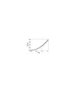
Figure 3: Dimensionless surface tension coefficient along the phase separation curve (numerical solution), $\sigma_{0}=\sqrt{\pi}\hbar^{2}g_{0}^{3}/2m_{B}a^{4}_{BB}$. Approximation, Eq. (6.3), is shown by the dashed curve.

It is expected that the surface tension coefficient will decrease as one departs from the phase separation curve. However near the transition line this change is not significant compared to the change in the bulk energy. Therefore to estimate nucleation rates it is sufficient to use Eq. (6.3). The bulk energy is given by the integral of $E(\rho)$ over the volume of the bubble. Therefore $\rho_{0}\Delta\mu$ is the energy difference $\Delta\mu\rho_{0}\equiv E(\rho_{0})-E(0)$ or the degree of metastability, see Fig. 1c. When $n_{F}\to n_{F}^{0}$, $\Delta\mu$ vanishes and therefore along the large part of the phase separation curve $\Delta\mu\sim\Delta n_{F}$. However, this in not the case near the end of the curve when $n_{F}^{0}\to 0$. Generally,

$$\frac{\Delta\mu a_{BB}^{3}}{\lambda_{BF}g_{1}^{2}}=K\Delta n_{F}+K^{\prime}\left[\frac{3}{2}(n_{F}^{2/3}n_{F,2}^{0\,1/3}-n_{F}^{0})-\Delta n_{F}\right]$$ (6.4)

where

$$K^{\prime}=\frac{2}{3}\frac{(n_{F}^{0\,2/3}+n_{B})^{3/2}}{n_{B}n_{F}^{0\,1/3}}\quad\quad K=K^{\prime}-\frac{2}{3}\frac{n_{F}^{0\,2/3}}{n_{B}}-1$$ (6.5)

One can see that when $\Delta n_{F}\ll n_{F}^{0}$ the second term in Eq. (6.4) vanished and we can use $\Delta\mu\sim K\Delta n_{F}$ as pointed out earlier. In the opposite case $K\sim K^{\prime}\to 2n_{B}^{1/2}/3n_{F}^{0\,1/3}$ and $\Delta\mu\sim n_{B}^{1/2}\Delta n_{F}^{2/3}$. In this last limit, however, one has to account for renormalization of the boson kinetic term and, thus, the surface tension coefficient $\sigma$, as discussed earlier.

The phase transition and formation of the fermion droplet is due to the interplay between the surface tension and bulk energy of the droplet [the last two term in $S$, see Eq. (6.1)], which creates a potential barrier. The system (instanton) has to tunnel through this barrier creating the critical droplet of radius $R_{c}=3\sigma/\rho_{0}\Delta\mu$. The rate of such the nucleation process is found from $\delta S/\delta R=0$, with the result $\ln\Gamma/\Gamma_{0}=-5\pi^{2}\sqrt{m_{B}\rho_{0}\sigma}R_{c}^{7/2}/2^{9/2}\hbar^{2}$. In terms of dimensionless densities of Fig. 1a, for $\Delta n_{F}\ll n_{F}^{0}$ we obtain

$$\ln{\Gamma^{\prime}/\Gamma_{0}}=-0.0056\frac{n_{B}^{11/2}}{g_{B}K^{7/2}}\left({n_{F}^{s}\over\Delta n_{F}}\right)^{7/2}.$$ (6.6)

Here $g_{B}$ is the conventional boson gas parameter as define earlier.

As expected, the tunneling exponent, i.e. the rhs of Eq. (6.6), is singular in the degree of metastability $\Delta n_{F}$ and diverges as $\Delta n_{F}^{-7/2}$. Equation (6.6) also indicates that the rate of nucleation is exponentially small in the dilute limit, i.e., for $g_{B}\ll 1$. Since the thin wall approximation (nucleation) requires sufficiently high energy barrier, e.g. Fig. 1(b,c), the rhs of Eq. (6.6) can not be reduce significantly decreasing $n_{B}$, see Eq. (4.7) and Fig. 2a. However, due to the smallness of the numerical coefficient one can hope that quantum nucleation is observable in sufficiently strongly coupled systems (which are presently realizable with the use of Feshbach resonance). Indeed, for $g_{B}\sim 0.1$, $n_{B}\sim 0.4$, and $\Delta n_{F}/n_{F}^{s}=0.15$, the coefficient $K\sim 0.27$ and the tunneling exponent, is $\sim-27$. For the same parameters and $a_{BB}\sim 20$ a.u. the estimate of the prefactor $\Gamma_{0}/V$ gives $10^{11}$ s${}^{-1}\mu$m^-3. As the result the nucleation rate $\Gamma/V$ is of the order $1$ s${}^{-1}\mu$m^-3. This is readily observable.

Let us now include dissipation terms (5.2). Exact evaluation of extremal action $S+\Delta S$, Eqs. (6.1) and (5.2), is not possible and we use the variational technique. A natural anzats is $R(t)=pR_{c}e^{-\alpha t^{2}}$, where coefficients $\alpha$ and $p$ are variational parameters. The expression for $\Delta S$, Eq. (5.2), does not depend on the time scale of $R(t)$. Rescaling of $R(t)$ yields $\Delta S\sim p^{4}R_{c}^{4}$. The proportionality coefficient depends only on the shape of the trial function, and, thus, can be estimated separately. The system $\partial_{p}(S+\Delta S)=0$, $\partial_{\alpha}S=0$ leads to the solution

$$p=\frac{{75\sqrt{6}\gamma^{2}+42\sqrt{10}\pi+15\gamma\sqrt{150\gamma^{2}+7\sqrt{15}\pi}}}{{300\gamma^{2}+32\sqrt{15}\pi}}$$ (6.7)

where for $\Delta n_{F}\ll n_{F}^{0}$

$$\gamma=0.742g_{0}^{1/5}n_{B}\left(\frac{m_{F}}{m_{B}}\right)^{4/5}\sqrt{\frac{n_{F}^{s}}{K\Delta n_{F}}}$$ (6.8)

Note that $p\to 7\sqrt{3}/8\sqrt{2}$ for $\gamma\to 0$ and $p\to\sqrt{3/2}$ for $\gamma\to\infty$. The second limit gives the leading asymptotic in the vicinity of the phase separation curve

$$\ln\Gamma^{\prime\prime}/\Gamma_{0}\sim-0.01\frac{n_{B}^{32/5}}{g_{B}^{4/5}K^{4}}\left({m_{F}\over m_{B}}\right)^{4/5}\left(n_{F}^{s}\over\Delta n_{F}\right)^{4},$$ (6.9)

The other limit gives expression (6.6) with slight overestimate of the numerical prefactor due to variational nature of the calculation. The overall solution is

$$\frac{\ln\Gamma/\Gamma_{0}}{\ln\Gamma^{\prime}/\Gamma_{0}}=\!\left(\frac{8\sqrt{2}}{7\sqrt{3}}\right)^{\!\!\!7/2}\!\!\left[\!\sqrt{8}p^{7/2}\sqrt{1\!-\!\sqrt{\!\frac{2}{3}}p}+\!\gamma\frac{5^{3/4}2^{1/4}}{\sqrt{\pi}}p^{4}\right]$$ (6.10)

where we have rescaled the overall numerical coefficient to mach expression (6.6) in the underdamped limit $\gamma\to 0$. The exponent $\ln\Gamma/\Gamma_{0}$ as a function of $\Delta n_{F}/n_{F}^{s}$ is shown in Fig. 4.

The crossover between power $4$ and $7/2$ asymptotic curves take place at $\gamma\sim 1$, or

$$K\Delta n_{F}/n_{F}^{s}\sim g_{B}^{2/5}n_{B}^{9/5}\left(\frac{m_{F}}{m_{B}}\right)^{8/5}$$ (6.11)

Thus, we find that correction due to dissipation term, $\Delta S$, strongly alters the tunneling exponent in the region $K\Delta n_{F}/n_{F}^{s}\!\!\ll\!g_{B}^{2/5}n_{B}^{9/5}(m_{F}\!/m_{B})^{8/5}$, while in the opposite (non-dissipative) limit the tunneling exponent is given by Eq. (6.6). From Eqs. (6.9) and (6.11) we conclude that the influence of dissipation is significant for large $m_{F}/m_{B}$ mass ratio. From the crossover condition we also see that the dissipative regime is realized near the phase separation curve within a “band” of width $\Delta n_{F}$ determined by the relation (6.11). For mixtures with small fermion-boson mass ratio this “band” is relatively narrow and for large enough fermion density the system stays in non-dissipative regime, where the nucleation rate is given by Eq. (6.6).

Let us consider the previous example (with $g_{B}\sim 0.1$, $n_{B}\sim 0.4$, etc.) assuming $m_{F}=m_{B}$. For this set of parameters the system is in the crossover region (at the edge of the dissipative “band” on the phase diagram). Using Eq. (6.10) we obtain $\ln\Gamma/\Gamma_{0}\sim-70$, which means that the transition is not observable. Choosing a smaller mass ratio, e.g. $m_{F}/m_{B}\sim 1/4$ (the right-hand side of Eq. (6.11) becomes smaller by an order of magnitude), we shrink the dissipative region around the phase transition curve. The system now is in “quiet” (non-dissipative) regime and the previous estimates for the rate obtained with Eq. (6.6) are valid. Therefore the dynamics of quantum nucleation can be systematically observable only for cold atom systems with sufficiently small mass ratio $m_{F}/m_{B}$.

VII Tunneling near spinodal instability

In this section we evaluate the transition rate near the absolute instability line, i.e. $n_{F}^{s}-n_{F}\ll n_{F}^{s}$. In this case the barrier separating the metastable mixture becomes small, see Fig. 1c, curve Y. To compute the tunneling part of the transition based on action (4.4) it is sufficient to retain only a few terms in the expansion of $E(\rho)$ at $\rho\to\rho_{0}$. The terms of the second and the third order in $\delta\rho=\rho-\rho_{0}$ will form the barrier (we set $E(\rho_{0})=0$ for convenience). It is clear that in the kinetic part of the action only the second order terms should be kept (the third order terms containing gradients are small compared to the third order potential terms). We obtain

$$S=4\pi\int dtdrr^{2}\left[\frac{m_{B}}{2\rho_{0}}\left(\frac{1}{r^{2}}\int_{0}^{r}dr^{\prime}{r^{\prime}}^{2}\partial_{t}\delta\rho\right)^{2}\right.$$ (7.1)

$$\left.+\frac{\hbar^{2}}{8m_{B}}\frac{\left(\nabla\delta\rho\right)^{2}}{\rho_{0}}+a\delta\rho^{2}+b\delta\rho^{3}\right],$$

where

$$a={2\pi\hbar^{2}a_{BB}\over{3m_{B}}}\left(1-{n_{F}\over n_{F}^{s}}\right)$$

and

$$b={\hbar^{2}a_{BF}^{5}m_{B}\over 3a_{BB}m_{F}^{2}}\left(1+{m_{F}\over m_{B}}\right)^{5}.$$

The dependence of action (7.1) on $n_{F}$ and $n_{B}$ can be obtained rescaling $r$, $t$, and $\delta\rho$, similarly to Ref. LifshitzKagan, . By introducing dimensionless variables Ls-note $x=r\sqrt{8m_{B}\rho_{0}a}/\hbar$, $\tau=4\rho_{0}at/\hbar$, and $p=\delta\rho b/a$, the action $S$ can be rewritten as $const\times s$, where $s[p(x,\tau)]$ is a parameter-independent functional, the extremum of which is a c-number. Its value can be estimated by variational anzats $p=-p_{0}\exp{(-\alpha x^{2}-\beta\tau^{2})}$, where $\alpha$, $\beta$ and $p_{0}$ are variational parameters. We find $\alpha=\beta=4/3$, $p_{0}=9$, and $s\approx 8.95$. Upon a straightforward calculation one obtains

$$\ln{\Gamma_{Y}/\Gamma_{0}}=-{0.324\over g_{B}n_{B}^{2}}\left(1-{n_{F}\over n_{F}^{s}}\right)^{1/2},$$ (7.2)

Again we see that tunneling exponent is controlled by the inverse boson gas parameter $g_{B}$.

The exponent vanishes when fermion density $n_{F}$ reaches the instability line $n_{F}^{s}$, where effective energy barrier disappears, see Fig. 1c. In this case the transition rate is defined by the prefactor $\Gamma_{0}/V$ rather then exponent, which is especially troublesome for a dense system. This limit, however, is not of interest here. Moreover, for not very small $n_{B}$ the observable transition occurs much closer to the phase separation curve (far from the instability point) and is described by Eq. (6.10) of Sec. VI.

When $g_{B}\lesssim 0.01$ and $n_{B}\sim 0.1-1$, the phase transition is not observable near the transition curve, see Eqs. (6.6) and (6.9),—one has to chose the values of $n_{F}$ closer to the spinodal instability. In this case the exponent (7.2) is significant. It rises rapidly as the function of $n_{F}^{s}-n_{F}$ defining the transition rate near the instability region. In this respect Eq. (7.2) is similar to the results on Macroscopic Quantum Tunneling (MQT) in systems of trapped bosons with attractive interactions UedaLeggett . When the coherence length $l_{s}$, see Eq. (4.8) is still much smaller then the size of the condensate, the height of the potential barrier and thus the tunneling exponent for the critical droplet are controlled not by the total number of particles in the trap, but the local densities. Therefore, for sufficiently large numbers of particles in the trap the tunneling exponent can be fine-tuned with a desired accuracy, which can make observation of the MQT rate possible in a well controlled and predictable regime.

The contribution of dissipation, e.g., action $\Delta S$ in Eq. (5.3), can be estimated by using the same variational anzats as above. Rewriting the integral in Eq. (5.3) in terms of $x$, $\tau$ and $p$ one finds that $\Delta S$ does not depend on $a$ and thus $n_{F}-n_{F}^{s}$. Therefore for large enough $n_{F}-n_{F}^{s}$ and small $g_{B}$ one can treat the dissipation perturbatively substituting $p(x,\tau)$ from the above calculations. As the result the tunneling exponent acquires an additional term $\sim-(g_{B}n_{B}^{2}m_{F}/m_{B})^{4/5}$. This term is again controlled by the mass ratio $m_{F}/m_{B}$. For not too high fermion/boson mass ratio, it is of the order $g_{B}$ and thus dissipation does not significantly alter the dynamics of the phase transition (MQT) in this region, see Fig. 4.

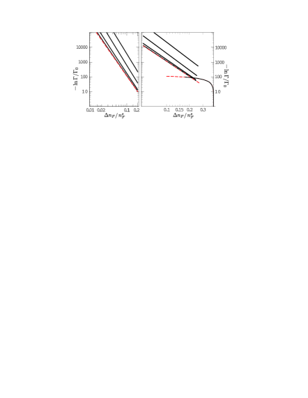
Figure 4: Transition rate exponent, $\ln\Gamma/\Gamma_{0}$, as a function of fermion density, $n_{F}=n_{F}^{0}+\Delta n_{F}$, for $n_{B}=0.4$, $g_{B}=0.1$ (left) and $g_{B}=0.01$ (right). Asymptotics near the i-ii phase separation curve are plotted for $m_{F}/m_{B}=0.01,0.1,1,10$ (solid curves, bottom to top). The dashed line represents the rate without dissipation, see Eq. (6.6). The asymptotic near the instability region, Eq. (7.2), is given in the right plot (for the same variation of $m_{F}/m_{B}$).

VIII Thermal nucleation

It is instructive to analyze the influence of the classical (thermal) activation mechanism. In order leave the metastable state finite temperature system can (in addition to direct tunneling leakage from its false “ground” state) use its entire spectrum tunneling from high energy states or going over the barrier. The rate of such transition is proportional to the sum LifshitzKagan ; Gorokhov of $\Gamma(E_{n})\exp[-(E_{n}-E_{0})/kT]$, where the prefactor accounts for possible tunneling from $n$-th exited state of the metastable mixture. This regime becomes effective when the largest energy gap—between the first exited and the ground state energies of the mixture—is of the order $k_{B}T$. This energy difference enters the expression for quantum nucleation rate and can be easily estimated in a similar manner

$$E_{1}-E_{0}\sim\frac{p^{2}}{2m_{B}}\sim\frac{1}{2m_{B}}\left(\frac{\hbar}{l}\right)^{2}.$$ (8.1)

Here the characteristic length scale is the coherence length of boson-fermion mixture.

Near the phase transition curve $l$ is given by Eq. (4.7), i.e. $l\sim a_{BB}/g_{0}n_{B}$. This gives the relation

$$g_{B}^{2}n_{B}\sim\frac{m_{B}a_{BB}^{2}k_{B}T}{\hbar^{2}}$$ (8.2)

Critical temperature of BEC transition can be estimate by that of the uniform non-interacting three-dimensional boson gas $k_{B}T_{c}\sim\hbar^{2}n_{B}^{2/3}/m_{B}$, and we finally obtain condition for thermal assisted transition in the form

$$g_{B}^{2/3}n_{B}\sim\frac{T}{T_{c}}$$ (8.3)

Our boson system is in deep BEC state, i.e. $T\ll T_{c}$, therefore thermal fluctuations are not significant for observable quantum nucleation that occurs in sufficiently dense systems ($n_{B}\sim 1$).

In dilute systems, where direct tunneling from low laying states is extremely slow, one has two compute the entire sum

$$\Gamma=\sum_{n}\Gamma_{0}(E_{n})e^{-S_{n}/\hbar-(E_{n}-E_{0})/kT}$$ (8.4)

up to the continuum states where $S_{n}\to 0$. The summation can be carried out semiclassically minimizing the new energy functional, i.e. exponent of Eq. (8.4), see e.g. Ref. LifshitzKagan, .

Closer to the spinodal instability the barrier becomes smaller and the tunneling is effective even for relatively dilute systems. For the crossover temperature we obtain

$$g_{B}^{2/3}(1-n_{F}/n_{F}^{s})\sim T/T_{c}.$$ (8.5)

In this case, as expected, the zero-temperature MQT mechanism can be observed in certain distance from the instability line, i.e. when the left-hand side of Eq. (8.5) is greater.

IX Expansion of supercritical droplet

As soon as a critical droplet is created as the result of tunneling or temperature fluctuations, it should grow equilibrating the system as pointed out in Sec. IV. Below we discuss only the case of finite coherent length—the situation when a distinct stable droplet is created (thin-wall approximation). We will estimate the expansion rate for $l\ll R_{c}\ll R$ in the limits of large and small dissipation.

After a given nuclei passes (tunnel trough) the energy barrier, its growth can be described by classical equation of motion for radius $R$, $\delta S/\delta R+f_{d}=0$. Here $f_{d}$ is the dissipative force (external time-dependent force is negligible at low temperatures), and the action $S$ should be formulated in real (original) time, i.e. in action (6.1) one replaces $it\to t$. In the underdamped limit, $f_{d}\to 0$ (energy conserved), the expansion is described by

$$\frac{{m_{B}\rho_{0}R^{3}}}{2}\left({\partial_{t}R}\right)^{2}=-\sigma R^{2}+\Delta\mu\frac{{\rho_{0}R^{3}}}{3}.$$ (9.1)

For large droplets ($R\gg R_{c}$) the surface tension term is negligible and the expansion is linear in time $R\simeq\alpha_{0}t$, with

$$\alpha_{0}=\sqrt{2\Delta\mu/3m_{B}}.$$ (9.2)

Fermion particle-hole excitations affect the the expansion dynamics, renormalizing the expansion rate $\alpha_{0}$. To estimate this effect we need to account for the dissipative part of the action. This can be done by analytical continuation of Matsubara action, Eq. (5.1), to Keldysh contour. Following Ref. Kamenev, we obtain

$$\Delta S=\frac{m_{F}^{2}\lambda_{BF}^{2}}{2\pi\hbar^{3}}\!\!\int\!\!dt\frac{d{\bf{q}}}{(2\pi)^{3}}\frac{1}{q}\dot{\rho}_{cl}(q,t)\rho_{q}(q,t)+\mathcal{O}(\rho_{q}^{2}(q,t)),$$ (9.3)

where $\rho_{cl/q}=(\rho_{+}\pm\rho_{-})/\sqrt{2}$ and $\rho_{\pm}$ resides on forward (backward) branch. In the nucleation limit (thin wall approximation) the time dependance of $\rho(\mathbf{r},t)$ enters only via radius of the droplet, $R(t)$, therefore $\rho_{\pm}=\rho\{R_{\pm}\}$. In the classical limit we keep only terms linear in $R_{q}$. The dissipative force becomes

$$f=\frac{m_{F}^{2}\lambda_{BF}^{2}}{2\pi\hbar^{3}}\!\!\int\!\!dt\frac{d{\bf{q}}}{(2\pi)^{3}}\frac{1}{q}\dot{\rho}_{cl}(q,t)\frac{\delta\rho_{q}(q,t)}{\delta R}.$$ (9.4)

Substitution of $\rho(\mathbf{r},t)=\rho_{0}\theta(r-R(t))$ will lead to the logarithmic divergence in the integration over the momentum. The divergence is due to the high $q$. The cutoff comes from the thickness of the surface area of the droplet. Using a more accurate expression for $\rho(\mathbf{r},t)$, i.e. Eq. (4.6), we obtain

$$f=-\gamma_{e}\gamma_{0}\dot{R}(t)R(t)^{2}\ln\frac{4R(t)}{\pi l},$$ (9.5)

where $\gamma_{e}=0.577...$ is the Euler constant, and $l$ is the coherence length. As the result, expansion of a large supercritical droplet is governed by

$$m_{B}\rho_{0}R\partial_{t}^{2}R + \frac{3m_{B}\rho_{0}}{2}(\partial_{t}R)^{2}$$

$$+ \gamma_{e}\gamma_{0}(\partial_{t}R)\ln\frac{4R}{\pi l}-\rho_{0}\Delta\mu=0.$$

This equation can be analyzed numerically for dimensionless variables. Define $t=t_{0}\tau$, $R(t)=R_{c}\chi(\tau)$, then Eq. (IX) becomes

$$-\chi\partial_{\tau}^{2}\chi-\frac{3}{2}(\partial_{\tau}\chi)^{2}-f_{0}(\partial_{\tau}\chi)\ln(\chi/{\xi})+1=0.$$ (9.7)

Here $f_{0}=\gamma_{e}\gamma_{0}t_{0}/m_{B}\rho_{0}R_{c}$, $\xi=\pi l/4R_{c}$, and $t_{0}^{2}=R_{c}^{2}m_{B}/\Delta\mu$. Numerical integration shows that for $f_{0}\gtrsim 1$ and $\tau\gtrsim 100f_{0}$ the first and the second terms remain smaller by several orders of magnitude. Therefore we can ignore this terms in such the limit. Moreover, we notice that logarithmic pre-factor of the third term does not change significantly for large supercritical droplets. Therefore with sufficient accuracy the growth is still linear in time $R(t)\simeq\alpha t\ln^{-1}{(4\alpha t/\pi l)}$ with

$$\alpha=\frac{\rho_{0}\Delta\mu}{\gamma_{e}\gamma_{0}},$$ (9.8)

One can notice that $f_{0}\sim 1/\sqrt{\Delta\mu}$ and therefore diverges at the phase separation curve. As the result, the above solution is valid near the phase separation line. When the system is placed farther away from the phase separation curve, $\Delta\mu$ increases and $f_{0}$ becomes smaller. In this case we have to retain the first two derivative terms in Eq. (9.7). It changes the asymptotic behavior. In the limit $f_{0}\to 0$ we arrive to Eq. (9.1) with the solution $R(t)\backsimeq\alpha_{0}t$, where $\alpha_{0}$ is given by Eq. (9.2).

Similar to nucleation, the expansion of a supercritical droplet is controlled by particle-whole excitations if the system is prepared within a certain “dissipative” region around the phase separation line, e.g., Sec. VI. For larger degree of supersaturation, dissipation is less effective. The “dissipative” region can be approximately estimated from condition $f_{0}(\Delta\mu)\gtrsim 1$. We should note that measurement of the growth rate does not necessarily require extremely dense systems in which nucleation is observable. Supercritical droplet can be created externally, e.g. by some laser fields or trapped atoms of different sort. For such initiated supercritical droplet the growth rate could be readily observable.

X Discussion

In the previous sections we have considered dynamics of the nuclei of a new phase (i.e., pure fermion phase) in the fermion-boson mixture in the metastable state. We have derived asymptotic expressions for the nucleation rates for the system in two regimes: in the regime of weak metastability, e.g., near the phase transition line (Sec. VI) and near the spinodal (absolute) instability.

Analysis of Sec. VI leads to the conclusion that in the vicinity of the phase transition line the nucleation dynamics is practically not observable for sufficiently dilute systems. e. g., with $g_{B}\ll 1$. It may appear that the dependence of Eqs. (6.6), (6.9), and (6.10) on $n_{B}$ contradicts to this statement. Indeed the transition rate decreases with $n_{B}$ if $\Delta n_{F}$ is kept constant. Such limit, however, is incorrect, since the nucleation condition $l_{0}\lesssim R_{c}$ in not satisfied, $l_{0}\sim 1/n_{B}$ (or $1/\sqrt{n_{B}}$ if $g_{B}$ is constant). Evaluating $R_{c}$ in terms of $\Delta n_{F}$ one obtains the condition on $\Delta n_{F}$ for which the asymptotes (6.6), (6.9), and (6.10) are valid. We have $R_{c}/a_{BB}=0.219(n_{B}^{3/2}\!\!/g_{B}K)(n_{F}^{s}/\Delta n_{F})$. In the limit $n_{B}\to 0$ it gives $\Delta n_{F}/n_{F}^{s}\lesssim n_{B}$ (where the densities are dimensionless, i.e. in units of Fig. 1a, as before). Therefore in $n_{B}\to 0$ limit the power $7/2$ and $4$ asymptotes are not measurable.

Measurable transition rates for dilute systems can be found closer to the instability region. In this case one enters a crossover between nucleation and MQT regimes. As an example, let us consider the mixture with the boson gas parameter $g_{B}\sim 0.01$. For $a_{BB}\sim 10$nm and about $10^{8}$ confined particles. This corresponds to the densities of the order $10^{14}$cm^-3 with size of the trapped condensate $\sim 100\mu$m. For this parameters the position of the metastable mixture on the phase diagram, Fig. 1a, is primarily defined by the ratio $a_{BB}/a_{BF}$, see Eqs. (3.3) and (3.4), and can be controlled by changing the scattering lengths. The transition rate is $\Gamma/V\sim x^{5}\exp(-x/g_{B}n_{B}^{2})$ where $x^{2}=1-n_{F}/n_{F}^{s}$, see Eqs. (7.2), (4.8). The change of the prefactor is not significant due to fast decay of the exponent form $x\gtrsim 0.1n_{B}^{2}$ (for smaller $x$ accurate evaluation of $\Gamma_{0}/V$ is necessary). Therefore we conclude that for $(n_{F}^{s}-n_{F})/n_{F}^{s}\gtrsim 0.01n_{B}^{4}$ and $n_{B}\lesssim 1$ the dependence of the exponent (7.2) on the densities is measurable. In this case the coherence length $l_{s}\gtrsim 1\mu$m. It rises for small $n_{F}^{s}-n_{F}$, however at $l_{s}\ll 100\mu$m (or $1-n_{F}/n_{F}^{s}\gg 10^{-4}$) the transition is still controlled by local densities.

We have also found, e.g. Sections V and VI, that dissipation can rather strongly alter the dependence of the nucleation rate in the vicinity of the phase transition line. While the results obtained in these sections are likely to be correct only quantitatively, they show that in the vicinity of the transition line excitation of particle-hole pairs in the Fermi sea plays crucial role. As a result the Thomas-Fermi approximation is inapplicable within the “band” controlled by the fermion-boson interaction strength as well as fermion-boson mass ratio; see Sec. VI.

Finally we considered the dynamics of supercritical droplets, i.e, the ones which have tunneled to the supercritical size. We have found that in the non-dissipative regime the radius of the droplet grows linearly with time with the expansion rate coefficient proportional to $\sqrt{\Delta n_{F}}$. In dissipative region, which occurs near the phase transition line, the situation is quite similar: up to logarithmic corrections the radii of the droplets still grow linearly with time, with rate now being dependent on friction coefficient, see Sec. IX.

Appendix A Density Profile

To analyze the shape of the condensate density function $\rho(r)$ of the bubble, i.e. the solution of Eq. (4.5), it is convenient to introduce dimensionless quantities as $x=r/{\mathfrak{r}}$, $\xi=t/{\mathfrak{t}}$, $\varepsilon=E/{\mathfrak{E}}$, $s=S/{\mathfrak{S}}$, $u=\rho\lambda_{BF}/\mu_{F}$, and write the action (4.4) in the form

$$s=\int d\xi x^{2}dx\left[\frac{1}{u}\left(\frac{1}{x^{2}}\int\limits_{0}^{x}x^{2}\partial_{\xi}udx\right)^{2}+\frac{\left(\partial_{x}u\right)^{2}}{u}+\varepsilon(u)\right]$$ (A.1)

with

$$\varepsilon(u)=-\left[5Au_{0}+\frac{5}{2}(1-u_{0})^{3/2}\right]u+\frac{5}{2}Au^{2}-(1-u)^{5/2}$$ (A.2)

where $u_{0}={\lambda_{BF}\rho_{0}}/{\mu_{F}}=1-y^{2}$, ${\mathfrak{t}}={\hbar}/{4\lambda_{0}\lambda_{BF}\mu_{F}^{3/2}}$, ${\mathfrak{r}}^{2}={\hbar{\mathfrak{t}}}/{2m_{B}}$, and ${\mathfrak{E}}=\lambda_{0}\mu_{F}^{5/2}$. Note that the parameters $A$ and $y$ (or $u_{0}$), introduced in Sec. III, are generally independent and define the position on the phase diagram via the same relation as in Eq. (3.5). The relation (3.6) between them defines the special case—the equilibrium state (residing on the phase separation curve).

Here we are after the time-independent part of the action $s$. In the current notation equation (4.5) reads

$$\partial_{x}^{2}\sqrt{u}+\frac{2}{x}\partial_{x}\sqrt{u}=\frac{1}{4}\frac{\partial\varepsilon(u)}{\partial{\sqrt{u}}}$$ (A.3)

Let us first discuss the case when the second term of the left-hand side is negligible (which is clearly the case near the phase transition curve). Equation (A.3) can, then, be simplified to

$$\partial_{x}u=\sqrt{u}\sqrt{\varepsilon(u)-\varepsilon(u_{0})},$$ (A.4)

noticing that $(\partial_{x}\sqrt{u})\partial_{\sqrt{u}}=\partial_{x}$. This is also the consequence of energy conservation at large $x$ corresponding to the static part of action $s$. The right-hand side of (A.4) is too complicated for the equation to be solved analytically. However, for the purpose of integration, $\varepsilon(u)-\varepsilon(u_{0})$ can be approximated in the range $u_{1}\leq u\leq u_{0}$, where $\varepsilon(u_{1})=\varepsilon(u_{0})=0$, as

$$\sqrt{\varepsilon(u)-\varepsilon(u_{0})}\approx 4{\mathfrak{W}}(u-u_{1})^{1/2}(u_{0}-u)$$ (A.5)

with

$${\mathfrak{W}}^{2}=\frac{\varepsilon(u_{m})-\varepsilon(u_{0})}{4^{2}(u_{m}-u_{1})(u_{0}-u_{m})^{2}}$$ (A.6)

Here $u_{1}<u_{m}<u_{0}$ and $u_{m}\sim(u_{1}+u_{0})/2$. This approximation is exact at $u=u_{m}$, i.e. close to the maximum of the right-hand side of Eq. (A.4) and therefore should lead to correct estimate of the characteristic length scale of $u(x)$. The maximal absolute deviation $\eta(u)\!\equiv\!1\!-\!4^{2}{\mathfrak{M}}^{2}(u\!-\!u_{1})(u_{0}\!-\!u)^{2}\!/[\varepsilon(u)\!-\!\varepsilon(u_{0})]$ occurs at $u\to u_{0}$ and $u\to u_{1}$ at the end of the i-ii separation curve ($u_{0}\to 1$), as can be easily verified numerically. At that point we obtain $\eta(u_{0})\approx 0.421$. The error vanishes at the limit of small barrier, i.e. near the instability line on the phase diagram. With this approximation Eq. (A.4) can be easily solved with the result

$$\exp\left[4{\mathfrak{W}}\sqrt{u_{0}}\sqrt{u_{0}-u_{1}}(x-const)\right]=$$ (A.7)

$$=\frac{{\left({\sqrt{u}+\sqrt{u_{0}}}\right)\left({\sqrt{uu_{0}}+\sqrt{u-u_{1}}\sqrt{u_{0}-u_{1}}-u_{1}}\right)}}{{\left({\sqrt{u}-\sqrt{u_{0}}}\right)\left({\sqrt{uu_{0}}-\sqrt{u-u_{1}}\sqrt{u_{0}-u_{1}}-u_{1}}\right)}}$$

Here the characteristic size of the bubble, $R$, enters into the constant of integration. The characteristic length-scale on the surface of the bubble (the coherence length) is

$$l=\frac{{\mathfrak{r}}}{{\mathfrak{W}}u_{0}\sqrt{1-u_{1}/u_{0}}}$$ (A.8)

where ${\mathfrak{r}}/a_{BB}=\sqrt{5/4}A^{3/2}/\sqrt{2\pi}g_{0}$.

In the vicinity of the i-ii separation curve $u_{1}\to 0$, $A$ is a function of $u_{0}$ according to Eq.(3.6), and we use $u_{m}=u_{0}/2$. Substitution to Eq. (A.6) yields

$${\mathfrak{W}}^{2}=\frac{{1-\left({1-u_{0}/2}\right)^{5/2}}}{{2u_{0}^{3}}}-\frac{{15}}{{16}}\frac{A}{{u_{0}}}-\frac{5}{8}\frac{(1-u_{0})^{3/2}}{u_{0}^{2}}$$ (A.9)

As the function of $u_{0}$, ${\mathfrak{W}}\sqrt{A}$ varies from $~{}0.1195$ to $0.1212$ with the mean value of $0.1203$ (the root-mean-square deviation is $0.0004$). Therefore near the i-ii separation curve with the same precision the coherence length, $l_{0}$, becomes

$$\frac{l_{0}}{a_{BB}}=\frac{1}{g_{0}n_{B}}$$ (A.10)

In the vicinity of spinodal instability $u_{0}-u_{1}\approx 2^{5}A^{2}(1-n_{F}/n_{F}^{s})/9$ as can be verified by expanding $\varepsilon$ in powers of $u_{0}-u_{1}$, and we use $u_{m}=(u_{0}+2u_{1})/3$. Substitution into Eq. (A.6) yields

$${\mathfrak{W}}^{2}=\frac{5u_{0}}{256\sqrt{1-u_{0}}}+{\cal O}(u_{0}-u_{1})$$ (A.11)

Therefore the coherence length, $l_{s}$, clearly diverges as $1/\sqrt{1-n_{F}/n_{F}^{s}}$. Collecting all dimensional factors we obtain

$$\frac{l_{s}}{a_{BB}}=\frac{\sqrt{3}}{g_{0}\sqrt{\pi n_{B}}}\left(1-\frac{n_{F}}{n_{F}^{s}}\right)^{-1/2}+{\cal O}\left(1-\frac{n_{F}}{n_{F}^{s}}\right)$$ (A.12)

In the above analysis we have ignored the first derivative term in Eq. (A.3). It is strictly speaking negligible only near the phase transition curve for large thin-boundary bubbles. In the instability region solution (A.7) will change. Nevertheless, the analysis of Eq. (A.3) shows taht the characteristic length scale still has to be inverse-proportional to $\mathfrak{M}u_{0}$ and incorporate the divergence of $1/\sqrt{1-u_{1}/u_{0}}$. Therefore relation (A.8) still holds. This can be demonstrated by expanding the right-hand side of Eq. (A.3) in terms of $1-u_{1}/u_{0}$. In the intermediate region, i.e. $0<u_{0}-u_{1}<u_{0}$, the order-of-magnitude agrement is expected since no other features are present, as can also be verified numerically.

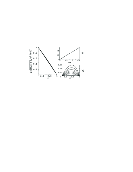
Figure 5: Normalized energy deviation, see Eq. (B.2), for $u_{0}=0.1,0.2,...,0.9$. Inset (a) gives absolute error of this expression with respect to a straight line approximation (for the same set of $u_{0}$). Inset (b) shows the relative error between the result of numerical integration in the lhs of Eq. (B.2) and ${\mathfrak{W}}u_{0}^{3/2}$ as a function of $n_{B}$ (solid line). The dashed line is a linear fit of the form $0.035n_{B}$.

Appendix B Surface Tension Near the Transition Curve

The surface tension has been defined as

$$\sigma=\sqrt{\frac{\hbar^{2}g_{0}^{2}{\mathfrak{E}}}{2m_{B}a_{BB}^{3}}}\frac{u_{0}^{1/2}}{2A}\int\limits_{0}^{1}{d\sqrt{z}}\sqrt{\varepsilon(u_{0}z)+1}$$ (B.1)

where we used the notations of Appendix A. Utilizing the approximation (A.5) at the i-ii transiiton curve, i.e. setting $u_{1}=0$, we obtain

$$\int\limits_{0}^{1}{d\sqrt{z}}\sqrt{\varepsilon(u_{0}z)+1}={\mathfrak{W}}u_{0}^{3/2}\left[1+\mathcal{O}(n_{B}/100)\right]$$ (B.2)

The left-hand side can be integrated numerically for various $u_{0}$ to verify the result, see Fig. 5. Significant relative error of Eq. (A.5) at $u\to u_{0}$ is suppressed in the above integral and the approximation (B.2) is accurate along the entire phase separation curve. Using the value of ${\mathfrak{M}}$ found earlier (see Appendix A) we finally obtain

$$\sigma=0.304\frac{\sqrt{\pi}\hbar^{2}}{2m_{B}a_{BB}^{4}}g_{0}^{3}n_{B}^{2}\left[1+\mathcal{O}(1/100)\right]$$ (B.3)

For large $n_{B}$, closer to “tricritical” point, the effective surface tension will deviate from the one obtained above due to additional gradient terms in Eq. (4.4). This is due to renormalization of the boson kinetic energy which is ignored by the Thomas-Fermi approximation. This correction is negligible for the parameters of interest, as explained in Sec. IV.

References

- (1) H. T. C. Stoof, J. Stat. Phys. 87, 1353 (1997); M. Ueda and A. J. Leggett, Phys. Rev. Lett. 80, 1576 (1998).
- (2) G. Roati, M. Zaccanti, C. D’Errico, J. Catani, M. Modugno, A. Simoni, M. Inguscio, and G. Modugno, Phys. Rev. Lett. 99, 010403 (2007).
- (3) I. M. Lifshitz and Yu. Kagan, Zh. Eksp. Teor. Fiz. 62, 385 (1972) [Sov. Phys. JETP 35, 206 (1972)].
- (4) I. M. Lifshitz, V. N. Polesskii, and V. A. Khokhlov, Zh. Eksp. Teor. Fiz. 74, 268 (1978) [Sov. Phys. JETP 47, 137 (1978)].
- (5) S. N. Burmistrov, L. B. Dubovskii, and V. L. Tsymbalenko, J. of Low Temp. Phys. 90, 363 (1993).
- (6) R. De Bruyn Ouboter, et al., Physica 26, 853 (1960); D. O. Edwards and J. G. Daunt, Phys. Rev. 124, 640 (1961); D. O. Edwards et al., Phys. Rev. Lett. 15, 773 (1965).
- (7) V. A. Mikheev et al., Phys. Low Temp. (U.S.S.R.) 17, 444 (1991); T. Satoh et al., Phys. Rev. Lett. 69, 335 (1992).
- (8) D. Solenov and D. Mozyrsky, Phys. Rev. Lett. 100, 150402 (2008).
- (9) A. G. Truscott et al., Science 291, 2570 (2001); M. W. Zwierlein et al., Phys. Rev. Lett. 92, 120403 (2004).
- (10) Y. Shin et al., Phys. Rev. Lett. 97, 030401 (2006).
- (11) Unlike in fermion-boson mixtures, phase separation transition in binary boson-boson systems corresponds to a continuous second order-like transition; see Ref. Timmermans,
- (12) E. Timmermans, Phys. Rev. Lett. 81, 5718 (1998).
- (13) G. D. Mahan, Many-Particle Physics (Kluwer Academic, New York, 2000).
- (14) L. Viverit, C. J. Pethick, and H. Smith, Phys. Rev. A 61, 053605 (2000).
- (15) D. Mozyrsky, I. Martin, and E. Timmermans, Phys. Rev. A 76, 051601(R) (2007).
- (16) H. Kleinert, Path Integrals in Quantum Mechanics, Statistics, Polymer Physics, and Financial Markets (World Scientific Publishing, 2004).
- (17) A. Imambekov, C. J. Bolech, M. Lukin, and E. Demler, Phys. Rev. A 74, 053626 (2006).
- (18) E. M. Lifshitz and L. P. Pitaevskii, Physical Kinetics, (Pergamon Press, 1981).
- (19) S. Coleman, Aspects of Symmetry (Cambridge University Press, 1985).
- (20) A. O. Caldeira and A. J. Leggett, Phys. Rev. Lett. 46, 211 (1981).
- (21) D. Solenov and V. A. Burdov, Phys. Rev. B 72, 085347, (2005);
- (22) D. Mozyrsky, I. Martin, A. Shnirman, and M. B. Hastings, cond-mat/0312503 at www.arXiv.org.
- (23) D. Solenov, Phys. Rev. B 76, 115309 (2007).
- (24) V. A. Burdov and D. Solenov, Int. J. of Nanoscience 6, 389 (2007).
- (25) Note that coincides with found earlier.
- (26) D. A. Gorokhov and G. Blatter, Phys. Rev. B 56, 3130 (1997).
- (27) A. Kamenev, cond-mat/0412296 at www.arXiv.org