Efficient diagrammatic computation method for higher order correlation functions of local type primordial curvature perturbations

Abstract

We present a new efficient method for computing the non-linearity parameters of the higher order correlation functions of local type curvature perturbations in inflation models having a $\cal N$-component scalar field, focusing on the non-Gaussianity generated during the evolution on super-horizon scales. In contrast to the naive expectation that the number of operations necessary to compute the $n$-point functions is proportional to ${\cal N}^{n}$, it grows only linearly in ${\cal N}$ in our formalism. Hence, our formalism is particularly powerful for the inflation models composed of a multi-component scalar field, including the models in which the slow-roll conditions are violated after the horizon crossing time. Explicit formulas obtained by applying our method are provided for $n=2,3,4$ and 5, which correspond to power-, bi-, tri- and quad-spectra, respectively. We also discuss how many parameters we need to parameterize the amplitude and the shape of the higher order correlation functions of local type.

I Introduction

Current observations of the cosmic microwave background (CMB) anisotropies indicate that primordial curvature perturbations are almost Gaussian Komatsu:2008hk . In general, if the perturbations are purely Gaussian, the statistical properties of the perturbations can be completely described by the two-point correlation function (=power spectrum). On the other hand, if the perturbations deviate from the Gaussian distribution, the non-Gaussianity affects the higher order correlation functions, or higher order spectra. Currently, the non-Gaussianity is attracting attention as a powerful probe to discriminate various inflation models Komatsu:2001rj ; Bartolo:2004if . In particular, there are a large number of studies on the three-point correlation function (=bi-spectrum). However, the four-point correlation function (=tri-spectrum) can also be constrained by future accurate measurements Okamoto:2002ik ; Bartolo:2005fp ; Kogo:2006kh ; D'Amico:2007iw . Using the analysis of both the bi-spectrum and the tri-spectrum in the future experiments, it is expected that we can extract more information about the mechanism of generating the primordial curvature perturbations. Hence, it is important to obtain useful formulas for the higher order correlation functions of primordial curvature perturbations.

Roughly speaking, the leading order of the connected part of $n$-point function is $O(P^{n-1})$, where $P\sim 10^{-10}$ is the amplitude of the power spectrum. Hence, it is naively expected to be difficult to measure higher order correlation functions. However, when the non-Gaussianity is large, this estimate $O(P^{n-1})$ will be replaced with $O(f_{{\rm NL}}^{n-2}P^{n-1})$ or even larger. Here, $f_{{\rm NL}}$ is a non-linearity parameter given in Refs. Komatsu:2001rj ; Bartolo:2004if ;

$$\zeta=\zeta_{G}+{3\over 5}f_{{\rm NL}}\zeta_{G}^{2}~{},$$ (I.1)

where $\zeta$ is the curvature perturbation on uniform energy density hypersurface and $\zeta_{G}$ is the linear Gaussian part. Notice that observationally $f_{{\rm NL}}$ can be as large as $O(100)$. This possible enhancement slightly improves the detectability of the higher order correlation functions. Furthermore, the number of argument wavenumbers of the $n$-point function is $n-1$. When the CMB temperature anisotropies, $C_{\ell}$, are measurable up to $\ell=\ell_{\rm max}$, the number of independent wavenumbers which we can measure will be roughly estimated as $\ell_{\rm max}^{2}$. Hence, the number of different combinations of argument wavenumbers increases as $\ell_{\rm max}^{2(n-1)}$. This large number enhances the effective amplitude of $n$-point function to $O(f_{{\rm NL}}^{-1}(f_{{\rm NL}}\ell_{max}P)^{n-1})$, while the amplitude of Gaussian noise is $O(P^{n/2})$. The detectability of the $n$-point function is basically determined by the ratio of these two numbers, $O\left(f_{{\rm NL}}^{-1}P^{-1/2}(f_{{\rm NL}}\ell_{max}\sqrt{P})^{n-1}\right)$. Hence, if $f_{{\rm NL}}\ell_{max}\sqrt{P}$ exceeds unity, all the higher order correlation functions are in principle measurable. For the Planck satellite :2006uk , it is expected that $\ell_{max}\sim O(2000)$. Hence, naively, if $f_{{\rm NL}}$ would be as large as $O(50)$, $f_{{\rm NL}}\ell_{max}\sqrt{P}$ can exceed unity. This fact strongly motivates a systematic derivation of the formulas for higher order correlation functions.

In this paper, we present a new method to calculate general $n$-point functions of local type primordial curvature perturbations. This new method is much more efficient than the straightforward calculations, especially when applied to the models with many components of inflaton field, including the models in which the slow-roll conditions are violated after the horizon crossing time. This method is based on the diagrammatic approach given in Ref. Byrnes:2007tm as well as on our previous work Yokoyama:2007uu ; Yokoyama:2007dw , in which the formulation for the bi-spectrum was developed. As for the parameterization of the higher order spectra, it is well known that the bi-spectrum can be parameterized by a single parameter, so-called non-linearity parameter, $f_{NL}$, while the tri-spectrum is parameterized by two parameters $\tau_{NL}$ and $g_{NL}$ Byrnes:2006vq due to the existence of two distinct terms that exhibit a different wavenumber dependence. That is, the number of parameters necessary to describe the higher order correlation functions is equal to the number of independent terms which have a different wavenumber dependence. Based on the diagrammatic method, we also show that one can easily count how many parameters we need to parameterize the amplitude and the shape of higher order spectra of local type.

This paper is organized as follows. In section II we briefly review the $\delta N$ formalism Starobinsky:1986fx ; Sasaki:1995aw ; Sasaki:1998ug ; Lyth:2004gb ; Lyth:2005fi , which is the foundation of our present analysis. We also discuss how many parameters we need to parameterize the higher order correlation functions. In section III we present our diagrammatic method for the computation of $n$-point correlation functions of primordial curvature perturbations. As an application of our method, in the succeeding section IV we give concise formulas for the power-, bi-, tri- and quad-spectra of the primordial curvature perturbations generated in multi-component inflation models. Section V is devoted to discussion and conclusion.

II local type primordial curvature perturbations and their parameterization

We focus on the non-Gaussianity generated during the evolution on super-horizon scales in multi-scalar inflation. We start with a brief review of the $\delta N$ formalism. Using the $\delta N$ formalism, we present a diagrammatic representation for general $n$-point functions of local type primordial curvature perturbations, and show how they are parameterized.

II.1 Background equations

We consider a ${\cal N}$-component scalar field whose action is given by

$$S=-\int d^{4}x\sqrt{-g}\left[{1\over 2}h_{IJ}g^{\mu\nu}\partial_{\mu}\phi^{I}\partial_{\nu}\phi^{J}+V(\phi)\right]~{},$$ (II.1)

$$\left(I,J=1,2,\cdots,{\cal N}\right)~{},$$

where $g_{\mu\nu}$ is the spacetime metric and $h_{IJ}$ is the metric on the scalar field space. In this paper we restrict our discussion to the flat field space metric $h_{IJ}=\delta_{IJ}$ to avoid inessential complexities due to non-flat field space metric, though the generalization is straightforward Yokoyama:2007dw .

We define $\varphi^{I}_{i}(i=1,2)$ as

$$\varphi^{I}_{1}\equiv\phi^{I}~{},~{}~{}\varphi^{I}_{2}\equiv\dot{\phi}^{I}~{},$$ (II.2)

where a dot ‘$`~{}\dot{}~{}$” represents differentiation with respect to the cosmological time.

For brevity, hereinafter, we use Latin indices at the beginning of Latin alphabet, $a$, $b$ or $c$, instead of the double indices, i.e., $X^{a}=X^{I}_{i}$. Then, the background equation of motion for $\varphi^{a}$ is

$${d\over dN}\varphi^{a}=F^{a}(\varphi)~{},$$ (II.3)

where $N$ is the $e$-folding number and $F^{a}(=F^{I}_{i})$ is given by

$$F^{I}_{1}={\varphi^{I}_{2}\over H}~{},~{}~{}F^{I}_{2}=-3\varphi^{I}_{2}-{V^{I}\over H}~{},$$ (II.4)

with $V^{I}=\delta^{IJ}(\partial V/\partial\phi^{J})$. The homogeneous background Friedmann equation is given by

$$H^{2}={1\over 3}\left({1\over 2}\varphi^{I}_{2}\varphi_{2I}+V\right)~{},$$ (II.5)

with $\varphi_{2I}=\delta_{IJ}\varphi^{J}_{2}$.

In the $\delta N$ formalism Starobinsky:1986fx ; Sasaki:1995aw ; Sasaki:1998ug ; Lyth:2004gb ; Lyth:2005fi , the difference in $e$-folding number between two adjacent background solutions describes the evolution of $\zeta$, curvature perturbations, on super-horizon scales. The solution of the background inflationary dynamics dominated by a ${\cal N}$-component scalar field is labelled by $2{\cal N}-1$ integration constants $\lambda^{a}$, besides the trivial time translation $\delta N$. Let us define $\delta\varphi^{a}$ as the perturbation,

$$\delta\varphi^{a}(\lambda;N)\equiv\varphi^{a}(\lambda+\delta\lambda;N)-\varphi^{a}(\lambda;N)~{},$$ (II.6)

where $\lambda$ is abbreviation of $\lambda^{a}$ and $\delta\lambda^{a}$ is a small quantity of $O(\delta)$.

2${\cal N}$ parameters $\{N,\lambda^{a}\}$ parameterize the initial values of fields. There is an arbitrariness in choosing the integral constants, i.e. a different choice of integration constants ${\bar{\lambda}^{a}}\equiv f^{a}(\lambda)$ is equally good. Here we leave the choice of $\lambda^{a}$ unspecified since all the discussion in the paper is not affected by the choice.

$\delta\varphi^{a}(N)$ defined by Eq. (II.6) represent perturbations of the scalar field on the $N={\rm constant}$ gauge Sasaki:1998ug . In this case, $\zeta$ at each point in space depends on the fluctuations of the scalar field at the same spatial point, and is given by

$$\zeta(N_{F},{\vec{x}})=\sum{1\over n!}N^{*}_{a_{1}a_{2\cdots}a_{n}}\delta\varphi^{a_{1}}_{*}({\vec{x}})\delta\varphi^{a_{2}}_{*}({\vec{x}})\cdots\delta\varphi^{a_{n}}_{*}({\vec{x}})~{},$$ (II.7)

$$N^{*}_{a_{1}a_{2\cdots}a_{n}}\equiv{\partial^{n}N(N_{F},\{\varphi^{a}\})\over\partial\varphi^{a_{1}}\partial\varphi^{a_{2}}\cdots\partial\varphi^{a_{n}}}\biggr{|}_{\varphi^{a}=\!{\stackrel{{\,{}_{(0)}}}{{\varphi}}}\!^{a}(N_{*})}~{}.$$

Here, the values of scalar fields on the initial flat hypersurface, $\{\varphi^{a}_{*}\}$, differ from place to place and characterize the initial perturbation. Since the e-folding number between the initial flat hypersurface and the final uniform energy density hypersurface depends on $\{\varphi^{a}\}$, as its argument we have used $\{\varphi^{a}\}$ instead of the initial time $N=N_{*}$. We have decomposed the scalar field as $\varphi^{a}=\!{\stackrel{{\,{}_{(0)}}}{{\varphi}}}\!^{a}+\delta\varphi^{a}$ and Taylor expanded $\zeta$ in terms of $\delta\varphi^{a}=O(\delta)$. The suffix $*$ represents the value evaluated at a certain time $N_{*}$ which is shortly after the horizon crossing time. The final hypersurface at $N=N_{F}$ is chosen to be an uniform energy density surface. As is well known, $\zeta(N_{F})$ is independent of the choice of $N_{F}$ as long as $N_{F}>N_{c}$, where $N_{c}$ is a certain time after the background trajectories have completely converged. According to the $\delta N$ formalism, the expansion coefficients $N^{*}_{a_{1}a_{2\cdots}a_{n}}$ are simply given by the derivatives of $N(N_{F},\{\varphi^{a}\})$, where $N(N_{F},\{\varphi^{a}\})$ is the $e$-folding number spent during the evolution of the homogeneous universe, in phase space, from the initial point $\{\varphi^{a}\}$ to the final uniform energy density surface.

II.2 Parameterization of the $n$-point functions

Let us begin with the two-point function. At the leading order in $\delta$,

the two-point function of $\zeta$ can be written as

$$\langle\zeta_{{\vec{k}}_{1}}\zeta_{{\vec{k}}_{2}}\rangle_{c} \equiv P_{\zeta}(k_{1})\delta^{(3)}({\vec{k}}_{1}+{\vec{k}}_{2})$$ (II.8)

$$= N_{a}N_{b}{\cal A}^{ab}(\vec{k}_{1})\delta^{(3)}({\vec{k}}_{1}+{\vec{k}}_{2})~{},$$

where $\langle\cdots\rangle_{c}$ means the expectation value of the connected part of “$\cdots$”, and we have abbreviated the suffix $*$. Here we have introduced the covariance matrix ${\cal A}^{ab}(\vec{k})$ defined by ${\cal A}^{ab}(\vec{k})\delta(\vec{k}+\vec{k}^{\prime})\equiv\langle\delta\varphi^{a}_{*\vec{k}}\delta\varphi^{b}_{*\vec{k}^{\prime}}\rangle_{c}$.

We assume that all the relevant components of the scalar field satisfy the slow-roll conditions at least until $N=N_{*}$, in which our formalism works quite efficiently. Otherwise, correlation functions can not be parameterized by a small number of parameters. In this case, $\{\delta\varphi^{a}_{*}\}$ is approximated by a set of Gaussian random variables with the scale invariant spectrum , and ${\cal A}^{ab}$ is given by ${\cal A}^{ab}=A^{ab}P(k)$ with

$$A^{IJ}_{11} \!\!= \!\!\delta^{IJ}~{},\qquad A^{IJ}_{12}=A^{IJ}_{21}=A^{IJ}_{22}=0~{},\qquad P(k)={2\pi^{2}\over k^{3}}\left({H_{*}\over 2\pi}\right)^{2}~{}.$$ (II.9)

Strictly speaking, even in the slow-roll inflation, $\delta\varphi^{a}_{*}$ deviates from pure Gaussian perturbation due to the effect of interaction. However, the non-Gaussianity of $\zeta$ caused by this deviation is suppressed by the slow-roll parameters, which is an undetectable level in the future experiments Seery:2006vu ; Seery:2006js ; Jarnhus:2007ia ; Arroja:2008ga . Hence, we neglect the non-Gaussianity of $\delta\phi^{I}_{*}$ here. In a similar fashion, the three-point correlation function at the leading order is given as Lyth:2005fi

$$\langle\zeta_{{\vec{k}}_{1}}\zeta_{{\vec{k}}_{2}}\zeta_{{\vec{k}}_{3}}\rangle_{c}=\frac{N^{a}N^{b}N_{ab}}{{(N_{c}N^{c})}^{2}}\left(P_{\zeta}(k_{1})P_{\zeta}(k_{2})+2~{}{\rm perms.}\right)\delta^{(3)}({\vec{k}}_{1}+{\vec{k}}_{2}+{\vec{k}}_{3})~{},$$ (II.10)

where $N^{a}\equiv A^{ab}N_{b}$. In deriving this equation, we have used $\langle\delta\varphi^{a}_{*{\vec{k}}_{1}}\delta\varphi^{b}_{*{\vec{k}}_{2}}\delta\varphi^{c}_{*{\vec{k}}_{3}}\rangle_{c}=0$. From this equation, we find that $\langle\zeta_{{\vec{k}}_{1}}\zeta_{{\vec{k}}_{2}}\zeta_{{\vec{k}}_{3}}\rangle_{c}$ is $O(\delta^{4})$. Since the wavenumber dependence of the bi-spectrum is completely given by the products of the power spectrum, the bi-spectrum is characterized by a single parameter $N^{a}N^{b}N_{ab}/{(N^{c}N_{c})}^{2}$, which controls the overall amplitude. Following literatures, we redefine the non-linearity parameter $f_{\rm NL}$ given in the introduction as Lyth:2005fi

$$f_{\rm NL}=\frac{5}{6}\frac{N^{a}N^{b}N_{ab}}{{(N_{c}N^{c})}^{2}}.$$ (II.11)

If only one field contributes to the curvature perturbation, $f_{\rm NL}$ defined by Eq. (II.11) is equivalent to Eq. (I.1). While Eq. (I.1) is valid only when the single field dominates the curvature perturbation, Eq. (II.11) can be applied to larger classes of inflation models where the curvature perturbations are sourced by multiple fields.

We can also write down the leading order four-point correlation function (the tri-spectrum) as Lyth:2005fi ; Byrnes:2006vq

$$\langle\zeta_{{\vec{k}}_{1}}\zeta_{{\vec{k}}_{2}}\zeta_{{\vec{k}}_{3}}\zeta_{{\vec{k}}_{4}}\rangle_{c}=\bigg{[}\frac{N^{a}N_{ab}N^{bc}N_{c}}{{(N_{d}N^{d})}^{3}}\left(P_{\zeta}(k_{1})P_{\zeta}(k_{12})P_{\zeta}(k_{4})+11~{}{\rm perms.}\right)$$

$$\hskip 85.35826pt+\frac{N^{a}N^{b}N^{c}N_{abc}}{{(N_{d}N^{d})}^{3}}\left(P_{\zeta}(k_{1})P_{\zeta}(k_{2})P_{\zeta}(k_{3})+3~{}{\rm perms.}\right)\bigg{]}\delta^{(3)}({\vec{k}}_{1}+{\vec{k}}_{2}+{\vec{k}}_{3}+{\vec{k}}_{4})~{},$$ (II.12)

where $k_{ij}\equiv|{\vec{k}}_{i}+{\vec{k}}_{j}|$ and $N^{ab}\equiv A^{ac}A^{bd}N_{cd}$. We see that the four-point function is $O(\delta^{6})$. Unlike the bi-spectrum, the tri-spectrum has two distinct terms that exhibit different wavenumber dependence. As a consequence, we need two parameters to specify the tri-spectrum. Following Ref. Byrnes:2006vq , we use the non-linearity parameters $\tau_{\rm NL}$ and $g_{\rm NL}$ defined by

$$\tau_{\rm NL}=\frac{N^{a}N_{ab}N^{bc}N_{c}}{{(N_{d}N^{d})}^{3}},~{}~{}~{}~{}~{}~{}~{}~{}g_{\rm NL}={25\over 54}\frac{N^{a}N^{b}N^{c}N_{abc}}{{(N_{d}N^{d})}^{3}}.$$ (II.13)

We can further proceed to higher order correlation functions. The main issue that we address in the rest of this section is how many parameters are necessary to parameterize the local type $n$-point function. Of course, we can count the number of such parameters by directly calculating the $n$-point function from Eq. (II.7) as in the case of the bi-spectrum or the tri-spectrum. Although in principle there are no difficulties in such a direct counting, the actual computation becomes exponentially more cumbersome as we proceed to higher order. Here, instead of resorting to the direct computation, we use a diagrammatic method Byrnes:2007tm .

The leading order of the $n$-point function consists of terms of $O(\delta^{2n-2})$, which are given by products of $(n-1)$ power spectra. According to the diagrammatic method, each of these leading terms has a corresponding connected diagram that consists of $n$ vertices and $(n-1)$ lines connecting two vertices. Such a connected diagram should have a tree structure. Namely, there is always a unique path that connects any pair of vertices in the diagram. We refer to such diagrams as reduced tree diagrams, to distinguish them from the (full) tree diagrams that will be introduced later.

The rules of the reconstruction of the leading term that constitutes the $n$-point function from a given reduced tree diagram are as follows Byrnes:2007tm . First, we assign a different wavenumber ${\vec{k}_{i}}(1\leq i\leq n)$ to each vertex $\bullet$ of the diagram, where ${\vec{k}_{1}},{\vec{k}_{2}},\cdots,{\vec{k}_{n}}$ are the arguments of the $n$-point function with the constraint ${\vec{k}_{1}}+{\vec{k}_{2}}+\cdots+{\vec{k}_{n}}=0$. Next we assign a wavenumber to each line in the diagram, too. In general, removing a line from the diagram yields two respectively connected sub-diagrams. Then, one assign to the removed line the sum of the vectors associated with all vertices in one of the two sub-diagrams. We do not care which of two sub-diagrams we choose since only the length of the assigned waved number is used in the following discussion. An example of the assignment of the wavenumber is given in Fig. 1.

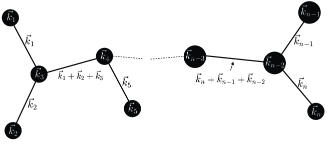
Figure 1: This figure shows the reduced tree diagram corresponding to one of the leading terms which constitute the $n$-point function whose arguments are ${\vec{k}_{1}},{\vec{k}_{2}},\cdots,{\vec{k}_{n}}$. The assignment of wavenumbers to the vertices and lines is illustrated.

After associating the wavenumbers with all lines, now we can assign the corresponding factors to the vertices and the lines. As for the vertex with $p$ lines attached, assign the factor $N_{a_{1}a_{2}\cdots a_{p}}$ to it. As for the lines, assign $A^{ab}P$, where the argument of the power spectrum $P$ is set to the length of the wavenumber associated with each line. By multiplying all these factors assigned to vertices and lines, and summing up all independent diagrams which are not mutually isomorphic, we obtain a function of $n$ wavenumbers, which constitutes the $n$-point function. The indices in $N_{a_{1}a_{2}\cdots a_{p}}$ assigned to each vertex are contracted with the indices of $p$ neighboring lines. Contraction is performed between lower and upper indices as usual.

Here, we did not associate a factor $1/p!$ with the vertex $N_{a_{1}a_{2}\cdots a_{p}}$ from the beginning for the following reason. A vertex with $p$ lines attached has $p$ lower indices to be contracted with the upper indices in $A^{ab}P$ associated with the $p$ attached lines. These $p$ lines are all to be distinguished because they are all labelled with different wavenumbers. Therefore there are $p!$ ways of contraction between two sets of $p$ indices. If we do not distinguish which indices are contracted, the factor $1/p!$ associated with the vertex is canceled.

Finally, by taking the sum over all the possible reduced tree diagrams, we obtain the $n$-point function. As an illustration, we show the diagrams for $n=3$ and $4$ in Figs. 2 and 3, respectively.

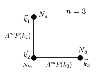
Figure 2: This diagram represents the leading term of the bi-spectrum of primordial curvature perturbations.

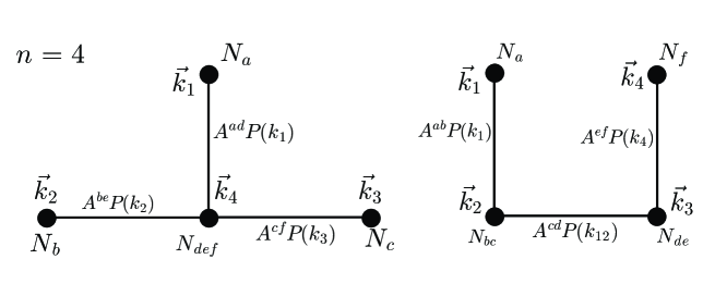
Figure 3: These diagrams represent the leading order terms of the tri-spectrum. These two distinct diagrams show different wavenumber dependence. Hence, two parameters are needed to describe the tri-spectrum.

It is not a trivial matter whether the functions constructed from two reduced tree diagrams that are not isomorphic to each other always yield a different functional dependence on the wavenumbers. As we explained in the appendix A, if the two reduced tree diagrams with $n$ vertices are not mutually isomorphic, the corresponding functions of $n$ wavenumbers are always different Ota . Therefore, the number of parameters necessary to determine the $n$-point function of $\zeta$ is equal to the number of independent reduced tree diagrams with $n$ vertices. As an illustration, we show in Table 1 the number of free parameters and the corresponding diagrams for $n=3,4,5$ and $6$.

A similar diagrammatic approach for the higher order correlation functions has been developed in the context of galaxy correlation or large scale structure. In Ref. Fry:1983cj , the author has given a numeration of the number of independent tree diagrams for general $n$, using the generating functions based on the combinatorial analysis Riorden:1958 . Applying this method to our discussion about the higher order correlation functions of the primordial curvature perturbations, we can find the number of independent reduced tree diagrams for general $n$, which corresponds to the number of free parameters for general $n$-point functions.

Table 1: This table shows the number of free parameters and the corresponding reduced tree diagrams for $n$-point correlation functions with $n=3,4,5,6$.

III A new method to compute $n$-point functions

In this section, we will provide an efficient method to compute the non-linearity parameters to characterize the $n$-point correlation functions.

III.1 tree-shaped diagrams

We start with the fact that $\zeta(N_{F})$ is independent of the choice of the time of the initial flat hypersurface $N_{*}$. By choosing $N_{*}$ to be identical to $N_{F}$ in (II.7), we obtain Lyth:2004gb

$$\zeta(N_{F}) = \sum{1\over n!}N^{F}_{a_{1}a_{2\cdots}a_{n}}\delta\varphi^{a_{1}}_{F}\delta\varphi^{a_{2}}_{F}\cdots\delta\varphi^{a_{n}}_{F}~{},$$ (III.1)

where $\delta\varphi^{a}_{F}=\delta\varphi^{a}(N_{F})$ are field perturbations evaluated on the flat slice at $N=N_{F}$. As we have mentioned in the previous section, $\zeta(N_{F})$ represents the curvature perturbation on the uniform energy density slice at $N=N_{F}$. Hence the above equation (III.1)means that the curvature perturbation $\zeta(N_{F})$ is simply caused by a time shift between the flat slice and the uniform energy density slice at the final time $N=N_{F}$. Hence, as shown in the appendix B, $N^{F}_{a_{1}a_{2\cdots}a_{n}}$ can be written only by local quantities at $N=N_{F}$. $N^{F}_{a_{1}a_{2\cdots}a_{n}}$ are therefore obtained immediately, once we specify $\varphi_{F}^{a}$.

What we need to evaluate is $\{\delta\varphi^{a}_{F}\}$ as functions of $\{\delta\varphi^{a}_{*}\}$. The evolution equations for $\delta\varphi^{a}$, which can be obtained by perturbing the background equation (II.3), are given by

$${d\over dN}\delta\varphi^{a}(N) \!= \!P^{a}_{~{}b}\delta\varphi^{b}(N)+{1\over 2}Q^{a}_{(3)bc}(N)\delta\varphi^{b}(N)\delta\varphi^{c}(N)+$$ (III.2)

$$\cdots+{1\over(\ell-1)!}Q^{a}_{(\ell)b_{1}b_{2}\cdots b_{\ell-1}}(N)\delta\varphi^{b_{1}}(N)\delta\varphi^{b_{2}}(N)\cdots\delta\varphi^{b_{\ell-1}}(N)+\cdots,$$

where $P^{a}_{~{}b}$ and $Q^{a}_{(\ell)b_{1}b_{2}\cdots b_{\ell-1}}$ are, respectively, defined by

$$\left.P^{a}_{~{}b}\equiv{\partial F^{a}\over\partial\varphi^{b}}\right|_{\varphi=\!{\stackrel{{\,{}_{(0)}}}{{\varphi}}}\!(N)}~{},~{}~{}Q^{a}_{(\ell)b_{1}b_{2}\cdots b_{\ell-1}}(N)\equiv{\partial^{\ell-1}F^{a}\over\partial\varphi^{b_{1}}\partial\varphi^{b_{2}}\cdots\partial\varphi^{b_{\ell-1}}}\biggr{|}_{\varphi=\!{\stackrel{{\,{}_{(0)}}}{{\varphi}}}\!(N)}~{}.$$ (III.3)

For the purpose of the evaluation of the $n$-point function, it is enough to truncate the expansion on the right hand side in Eq. (III.2) at $(n-1)$-th order. By solving the above equations from $N=N_{*}$ to $N_{F}$ with initial conditions $\delta\varphi^{a}(N_{*})=\delta\varphi^{a}_{*}$, we obtain $\delta\varphi^{a}_{F}$ expressed in terms of $\{\delta\varphi^{a}_{*}\}$. Due to the non-linear evolution after the horizon crossing, the distribution of $\{\delta\varphi^{a}_{F}\}$ is in general non-Gaussian even if that of $\{\delta\varphi^{a}_{*}\}$ is Gaussian.

If we solve the equations (III.2) iteratively, we can express formally $\delta\varphi^{a}_{F}$ as a Taylor expansion in terms of $\{\delta\varphi^{a}_{*}\}$. Let us denote the $m$-th order terms in the iterative expansion by $\delta\!{\stackrel{{\,{}_{(m)}}}{{\varphi}}}\!^{a}_{F}$. Then $\delta\varphi^{a}_{F}$ can be written as $\delta\varphi^{a}_{F}=\sum_{m=1}^{n-1}~{}\delta\!{\stackrel{{\,{}_{(m)}}}{{\varphi}}}\!^{a}_{F}$, where we truncate the expansion at the $(n-1)$-th order because higher order terms are irrelevant to the $n$-point function. By definition, $\delta\!{\stackrel{{\,{}_{(m)}}}{{\varphi}}}\!^{a}_{F}$ contains $m$ Gaussian random variables, $\{\delta\varphi^{a}_{*}\}$. Namely, there is a factor $\delta\varphi^{a_{1}}_{*}\cdots\delta\varphi^{a_{m}}_{*}$ in $\delta\!{\stackrel{{\,{}_{(m)}}}{{\varphi}}}\!^{a}_{F}$. The indices in this factor are to be contracted with the interaction vertices $Q^{a}_{(\ell)b_{1}b_{2}\cdots b_{\ell-1}}$ or the Green function $\Lambda^{a}_{~{}b}$, which obeys

$${d\over dN}\Lambda^{a}_{~{}b}(N,N^{\prime})=P^{a}_{~{}c}(N)\Lambda^{c}_{~{}b}(N,N^{\prime})~{},$$ (III.4)

$${d\over dN^{\prime}}\Lambda^{a}_{~{}b}(N,N^{\prime})=-\Lambda^{a}_{~{}c}(N,N^{\prime})P^{c}_{~{}b}(N^{\prime})~{}.$$ (III.5)

Here again an upper index is contracted with a lower index, as usual. All the possible ways of contraction contribute to $\delta\!{\stackrel{{\,{}_{(m)}}}{{\varphi}}}\!^{a}_{F}$.

We can associate a diagram as presented in Fig. 4 with each way of contraction. Hereinafter, we refer to such a diagram as a tree-shaped diagram, to distinguish it from the reduced tree diagram introduced earlier and from what is simply called a tree diagram which will be introduced later. A tree-shaped diagram is drawn obeying the following simple rules. We start with a solid circle $\bullet$ and attach a line downward to it. We attach an interaction vertex $\otimes$ to the other end of this line. From the vertex, several lines extend downward and they end with another interaction vertex $\otimes$ or a half open circle. This process is repeated until all the end points are terminated by a half open circle. The total number of half open circles should be $m$.

The solid circle $\bullet$ corresponds to $N_{a}^{F}$, and hence we assign the time $N=N_{F}$ to it. A half open circle corresponds to the initial Gaussian variables $\delta\varphi^{a}_{*}$, and hence the time $N=N_{*}$ is assigned to it. An interaction vertex $\otimes$ corresponds to the factor $Q^{b}_{(\ell)b_{1}\cdots b_{\ell-1}}(N)$, where $N$ ($N_{*}\leq N\leq N_{F}$) is the time assigned to this vertex and $\ell$ ($3\leq\ell\leq m$) is the number of attached lines. Here, we did not associate a factor $1/(\ell-1)!$ with $Q^{b}_{(\ell)b_{1}\cdots b_{\ell-1}}(N)$. The reason is the same as before in the case of $N_{a_{1}a_{2}\cdots a_{p}}$ discussed in Sec. II.2. Here, the half open circles are all supposed to be labelled, i.e. distinguishable. In this case dropping the factor $1/(\ell-1)!$ is exactly compensated by not distinguishing the order of lines attached to the same interaction vertex.

In this diagram the time flows from the bottom to the top as is indicated in Fig. 4. Finally, to each line segment, we assign the Green function (propagator) $\Lambda^{a}_{~{}b}(N,N^{\prime})$, where $N$ and $N^{\prime}$ are the time coordinates assigned to the upper and lower ends of the line, respectively. Contracting upper and lower indices between the adjacent objects (the solid circle, interaction vertices, half open circles and lines) and integrating over all the time coordinates assigned to the interaction vertices in the whole range of their possible variation, we obtain a quantity which constitutes $N_{a}^{F}\delta\!{\stackrel{{\,{}_{(m)}}}{{\varphi}}}\!^{a}_{F}$. Collecting all terms corresponding to different diagrams yields total $N_{a}^{F}\delta\!{\stackrel{{\,{}_{(m)}}}{{\varphi}}}\!^{a}_{F}$.

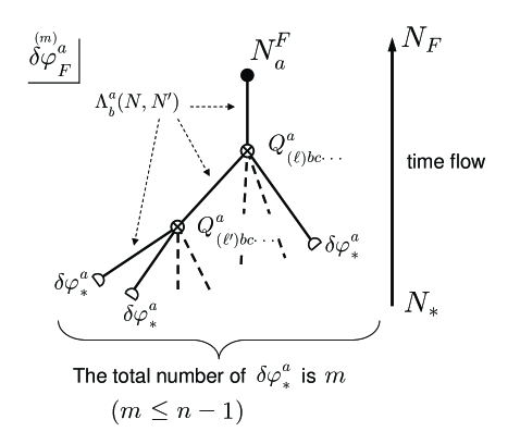
Figure 4: One example of tree-shaped diagram, which contributes to $\delta\!{\stackrel{{\,{}_{(m)}}}{{\varphi}}}\!^{a}_{F}$. The diagram branches off from the top to the bottom.

III.2 $n$-point correlation functions

Instead of $\zeta(N_{F})$, we first compute $n$-point functions of $\zeta^{(\rm lin)}_{F}$ defined by

$$\zeta^{(\rm lin)}_{F}=N_{a}^{F}\delta\varphi^{a}_{F},$$ (III.6)

which is the linear truncation of the Taylor expansion of $\zeta(N_{F})$ in terms of $\delta\varphi^{a}_{F}$. The $n$-point function of $\zeta^{(\rm lin)}_{F}$ is given by the sum of all the possible connected tree diagrams obtained by contracting all the half open circles $\{\delta\varphi_{*}^{a}\}$ in pair from a product of $n$ tree-shaped diagrams. (See Fig. 5.) Contraction between the half open circles within the same tree-shaped diagram can be neglected because it produces a loop. For the same reason, there is not more than one contraction between any pair of tree-shaped diagrams. Let us represent this contraction between a pair of half open circles, by a full open circle $\circ$, to which $A^{ab}$ defined in Eq. (II.9) is assigned. We refer to the diagram obtained by this contraction simply as a tree diagram. The leading terms of the $n$-point function of $\zeta^{(\rm lin)}_{F}$ are ${\cal O}(\delta^{2(n-1)})$, and hence the tree diagram should have $(n-1)$ open circles $\circ$. As any pair of tree-shaped diagrams does not have more than one contraction between them, all the half open circles belonging to a single tree-shaped diagram are contracted with different tree-shaped diagrams. Since all the tree-shaped diagrams are labelled with a different wavenumber $\vec{k}_{i}$, the assumption that all the half open circles are distinguishable holds. This contraction process does not produce any further statistical weight, and hence all the tree diagrams have the same weight of unity.

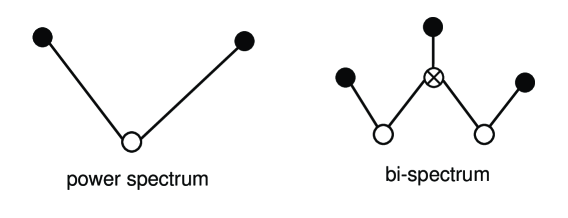
Figure 5: Tree diagrams corresponding to the power- and bi-spectra.

In addition to the linear term $\zeta^{(\rm lin)}_{F}$, $\zeta(N_{F})$ contains terms non-linear in $\delta\varphi^{a}_{F}$, which also contribute to the $n$-point functions of $\zeta(N_{F})$. There is one-to-one correspondence between the non-linear terms in $\zeta(N_{F})$ and the interaction vertex $\otimes$ that is directly connected to $\bullet$ by a line without any intervening vertices $\circ$ or $\otimes$. Hence, we can take into account this non-linear contribution simply by replacing the interaction vertices directly connected to $\bullet$ as

$$N^{F}_{a}\Lambda^{a}_{~{}c}(N_{F},N)Q^{c}_{(\ell)b_{1}\cdots b_{\ell-1}}(N)\longrightarrow N^{F}_{a}\Lambda^{a}_{~{}c}(N_{F},N)\hat{Q}^{c}_{(\ell)b_{1}\cdots b_{\ell-1}}(N)$$ (III.8)

$$\equiv N^{F}_{a}\Lambda^{a}_{~{}c}(N_{F},N)Q^{c}_{(\ell)b_{1}\cdots b_{\ell-1}}(N)+N^{F}_{b_{1}\cdots b_{\ell-1}}\delta~{}(N-(N_{F}-\varepsilon)),$$

where $\varepsilon$ is an infinitesimally small number. By this prescription, we can obtain the non-linearity parameters only from the tree diagrams.

Now we are ready to show that our method to evaluate the $n$-point functions can be reduced to the problem of solving the ordinary differential equations for vector variables that have only a single index $a$ ($1\leq a\leq 2{\cal N})$, which is the main result of this paper. Let us consider one tree diagram which constitutes the $n$-point function. We focus on one of sub-diagrams obtained by removing one vertex $\otimes$ or $\circ$ from a tree diagram, which we denote by $\Gamma_{a}$ or $\tilde{\Gamma}^{a}$. If the line which was attached to the removed object is pointing downward (upward), the vector has a lower (an upper) index. Suppose that the object attached to the other end of this line is an interaction vertex $\otimes$ with which $Q^{a}_{(\ell)b_{1}\cdots b_{\ell-1}}(N)$ associates. Let us consider the case of a vector $\tilde{\Gamma}^{a}$ with an upper index. Notice that the other lines connected to this vertex are also similar sub-diagrams which consist of smaller number of vertices than that we are focusing on. We denote the product of the vectors associated with all these sub-diagrams by a tensor $M^{c_{1}\cdots c_{\ell-1}}$. Those vectors appearing in $M^{c_{1}\cdots c_{\ell-1}}$ are already known by the induction assumption. Then, $\tilde{\Gamma}^{a}$ can be defined recursively as

$$\tilde{\Gamma}^{a}(N)=\int_{N_{*}}^{N}dN^{\prime}~{}\Lambda^{a}_{~{}b}(N,N^{\prime})Q^{b}_{(\ell)c_{1}\cdots c_{\ell-1}}(N^{\prime})M^{c_{1}\cdots c_{\ell-1}}(N^{\prime}).$$ (III.9)

From this equation, we find that $\tilde{\Gamma}^{a}(N)$ satisfies

$$\frac{d}{dN}\tilde{\Gamma}^{a}(N)=P^{a}_{~{}b}(N)\tilde{\Gamma}^{b}(N)+Q^{a}_{(\ell)c_{1}\cdots c_{\ell-1}}(N)M^{c_{1}\cdots c_{\ell-1}}(N).$$ (III.10)

The boundary conditions for $\tilde{\Gamma}^{a}(N)$ are set by $\tilde{\Gamma}^{a}(N_{*})=0$ at $N=N_{*}$, and hence the above equation is to be solved in the forward direction in time.

In the case of the vector with an upper index $\tilde{\Gamma}^{a}(N)$, the neighboring object can be $\circ$ instead of $\otimes$. In this case the initial conditions are given by $\tilde{\Gamma}^{a}(N_{*})=A^{ab}\Gamma_{b}(N_{*})$, where $\Gamma_{b}(N_{*})$ is the vector corresponding to the sub-diagram with the neighboring vertex $\circ$ being removed. The equation to solve is simply the homogeneous one given by

$${d\over dN}\Gamma_{a}(N)=-\Gamma_{b}(N)P^{b}_{~{}a}(N).$$ (III.11)

Similarly, for a vector $\Gamma_{a}$ with the neighboring object being $\otimes$, we have

$$\Gamma_{a}(N)=\int^{N_{F}}_{N}dN^{\prime}~{}\Lambda^{c_{1}}_{~{}a}(N^{\prime},N)\hat{Q}^{b}_{(\ell)c_{1}\cdots c_{\ell-1}}(N^{\prime})M_{b}^{~{}c_{2}\cdots c_{\ell-1}}(N^{\prime})~{},$$ (III.12)

and this vector obeys

$${d\over dN}\Gamma_{a}(N)=-\Gamma_{b}(N)P^{b}_{~{}a}(N)-\hat{Q}^{b}_{(k)ac_{2}\cdots c_{\ell-1}}(N)M_{b}^{~{}c_{2}\cdots c_{\ell-1}}(N)~{}.$$ (III.13)

The boundary conditions for $\Gamma_{a}(N)$ are set by $\Gamma_{a}(N_{F})=0$ at $N=N_{F}$, or equivalently $\Gamma_{a}(N_{F}-\epsilon)=N_{ac_{2}\cdots c_{\ell-1}}$ $M^{c_{2}\cdots c_{\ell-1}}(N_{F})$ taking into account the $\delta$-function term in the definition of $\hat{Q}^{c}_{(\ell)b_{1}\cdots b_{\ell-1}}$ in Eq. (III.8) as boundary conditions. In this manner, the effect of the non-linear terms in $\zeta(N_{F})$ in (III.1) can be absorbed by the boundary conditions in general. The equation is solved backward in time. There is another case in which the neighboring object is $\bullet$. This simplest case can be also handled in a similar manner. We defer its explanation to the succeeding section, where we exhibit some more explicit formulas. In Table 2, we summarize the notation of the vector quantities which will be used below, showing the correspondence to the tree-shaped diagram.

Table 2: This table shows the summary of the correspondence between the vector quantities used in this paper.

To obtain an expression for the $n$-point function written in terms of such vectors, we arbitrarily choose one vertex $\otimes$ or $\circ$ from a tree diagram at the beginning. Suppose that the chosen vertex is an interaction vertex $\otimes$ with which $Q^{a}_{(\ell)b_{1}\cdots b_{\ell-1}}(N)$ associates. After preparing all the necessary vectors, $\Gamma_{a}$ and $\tilde{\Gamma}^{b_{i}}_{(i)}$ $(1\leq i\leq\ell-1)$, which correspond to the sub-diagrams obtained when this vertex is removed, we can immediately write down the contribution to the $n$-point function from this tree diagram as

$$\int^{N_{F}}_{N_{*}}dN~{}\Gamma_{a}(N)Q^{a}_{(k)b_{1}\cdots b_{\ell-1}}(N)\prod_{i=1}^{\ell-1}\tilde{\Gamma}^{b_{i}}_{(i)}(N)~{}.$$ (III.14)

If the vertex which we initially focused on is $\circ$, with which $A^{ab}$ associates, we do not need the final integration over $N$. We denote the vectors that correspond to the sub-diagrams obtained by removing this $\circ$ by $\Gamma^{(1)}_{a}$ and $\Gamma^{(2)}_{b}$. Then, we compute

$$A^{ab}\Gamma^{(1)}_{a}(N_{*})\Gamma^{(2)}_{b}(N_{*}),$$ (III.15)

instead of the expression (III.14). In this diagrammatic method, the final expression for the spectrum in appearance depends on which vertex we chose at the beginning, but, of course, all different looking expressions are equivalent. Practically, it is more efficient to choose a vertex near the center so as to reduce the number of necessary vectors, although the definition of the center of a diagram is not so clear in many cases.

III.3 Relation to the reduced tree diagrams and statistical weight

As we mentioned in Sec. II.2, the reduced tree diagram is useful to classify the wavenumber dependence of the $n$-point functions, while the (full) tree diagram is a powerful tool for explicit computation of the $n$-point functions. We show that the reduced tree diagram introduced in Sec. II.2 is actually a simplified version of the tree diagram. It will be manifest that the solid circles attached to the ends of diagrams have the same meaning in both diagrams. In the reduced tree diagram the internal lines represent power spectrum of the initial Gaussian random field $\{\delta\varphi_{*}^{a}\}$, which is expressed by an open circle $\circ$ in the tree diagram. Hence, each line in the reduced tree diagram corresponds to a line with an open circle $\circ$ in the tree diagram. The sub-structure described by the interaction vertices $\otimes$ in the tree diagram is completely abbreviated in the reduced tree diagram. Hence, there is a degeneracy such that different tree diagrams contribute to the same reduced tree diagram. As explained in Sec. II.2 and proven in appendix A, the wavenumber dependence of the $n$-point functions is classified by the topology of the reduced tree diagram. This means that plural tree diagrams can give the contribution to $n$-point function with the same wavenumber dependence.

In Fig. 6, as an example, we show the diagrams corresponding to the tri-spectrum coefficient $g_{NL}$. We can decompose the top-left reduced tree diagram into 4 sub-diagrams by cutting all lines off. These sub-diagrams are counter parts of the tree-shaped diagrams. The lower part of this figure explains correspondence between these sub-diagrams and the tree-shaped diagrams. There are two tree-shaped diagrams with four half open circles as is explicitly shown in this figure. Hence, we find that the formula for $g_{NL}$ is composed of two different terms.

When we consider the statistical weight of the diagram, this correspondence between the reduced and full tree diagrams is important. The starting point is the fact that the statistical weight of each tree diagram is unity when each end point $\bullet$ is labelled by the assigned momentum. Therefore counting the statistical weight by writing down all different tree diagrams is straightforward. However, the non-linearity parameters are defined based on the reduced tree diagram. The most of the patterns which occur as a result of permutation of the momenta assigned to the end points $\bullet$ is taken care already in the definition of the non-linearity parameters. (See Eqs. (II.10) and (II.12).) However, here we should notice that some of the half open circles in the tree-shaped diagrams can be distinguishable, while the sub-diagrams obtained from the reduced tree diagram as mentioned above do not distinguish their legs at all. Therefore when there are several distinguishable patterns to assign the labels to the half open circles in a tree-shaped diagram, the term containing such a tree-shaped diagram has a factor corresponding to the number of patterns.

As an example, we again consider the case of $g_{NL}$. The tree-shaped diagram that has two three-point interaction vertices shown in Fig. 6 has three distinguishable patterns in assigning the labels $\{1,2,3\}$ to the three half open circles. This means that we need to add the corresponding factor $3$ to the contribution containing this tree-shaped diagram. (See the expression in Eq. (IV.6) below.)

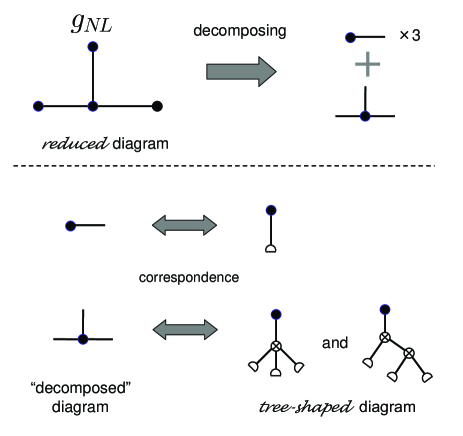
Figure 6: This figure shows the relation between the tree-shaped diagram and the reduced diagram for the non-linearity parameter $g_{NL}$. The upper one shows how to decompose the reduced diagram, and the lower one shows the correspondence between the ”decomposed” diagrams and the tree-shaped diagrams.

We want to emphasize that the above formulation simplifies the computation of higher order correlation functions a lot. In this formulation, we have only to solve vector quantities with only one index. Therefore our computation scheme requires the number of operations proportional to ${\cal N}$ in computing the non-linearity parameters in $n$-point function. If we performed a naive straightforward calculation, in which the derivatives of the $e$-folding number $N$ are computed by using the finite difference method numerically, the required number of operations is proportional to ${\cal N}^{n}$. If we naively performed perturbative expansion, in which we connect the interaction vertices by propagators $\Lambda^{a}_{~{}b}(N,N^{\prime})$ and perform integration over the time coordinates of the interaction vertices, the necessary number of operations would be even larger. When the number of inserted interaction vertices is $m$, naively we need $O({\rm several}~{}\times~{}{\rm(number~{}of~{}time~{}steps)}^{m})$ operations to compute the contribution of the single diagram. On the other hand, in our formulation we need only $O({\rm several}~{}\times~{}{\rm(number~{}of~{}time~{}steps)}~{}\times(m+{\rm a~{}few}))$ operations. Therefore our scheme is particularly useful for the computation of higher order correlation functions in the inflation models with a large number of field components.

IV Examples

In this section we apply our formalism to the computation of the power-, bi-, tri- and quad-spectrum to demonstrate the efficiency of our method.

IV.1 Power spectrum

Let us first consider the power spectrum. There is only one tree diagram that contributes to the power spectrum, which is shown on the left hand side in Fig. 5. Following the prescription given in the previous section, we focus on a unique vertex $\circ$.

Then, we can decompose this tree diagram into this open circle, with which $A^{ab}$ associates, and two identical sub-diagrams shown on the right hand side in Fig. 7. Corresponding to this simplest sub-diagram, we introduce a vector $N_{a}(N)$, whose explanation was deferred in the preceding section. This vector is defined by the equation

$$\frac{d}{dN}N_{a}(N)=-P^{b}_{~{}a}(N)N_{b}(N),$$ (IV.1)

with the boundary conditions $N_{a}(N_{F})=N_{a}^{F}$. The vector $N_{a}(N)$ represents the derivatives of the $e$-folding number with respect to $\varphi^{a}$ evaluated at $\varphi^{a}=\!{\stackrel{{\,{}_{(0)}}}{{\varphi}}}\!^{a}(N)$. Using this vector, the power spectrum of $\zeta(N_{F})$ is expressed as Yokoyama:2007dw

$$\frac{P_{\zeta}}{P}=A^{ab}N_{a}(N_{*})N_{b}(N_{*})\equiv W_{*},$$ (IV.2)

where $P_{\zeta}$ and $P$ are those which have already appeared in Eq. (II.8).

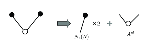
Figure 7: This figure shows how we decompose the tree diagram for the power spectrum, when we focus on the vertex $\circ$.

IV.2 Bi-spectrum

Just like the power spectrum, there is only one tree diagram that contributes to the bi-spectrum, which is presented on the right hand side in Fig. 5. Let us focus on the interaction vertex $\otimes$ to which $Q^{a}_{(3)bc}(N)$ is assigned, and decompose the diagram into the chosen vertex $\otimes$, a sub-diagram denoted by $N_{a}(N)$ and the two same sub-diagrams denoted by $\tilde{N}^{a}(N)$ as illustrated in Fig. 8.

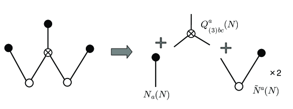
Figure 8: This figure shows how we decompose the tree diagram for the bi-spectrum, when we focus on the interaction vertex $\otimes$.

The sub-diagram denoted by $\tilde{N}^{a}(N)$ is reduced to that denoted by ${N}_{a}(N)$ if we remove one open circle $\circ$. Hence, following the general rule explained in the preceding section, the new vector $\tilde{N}^{a}(N)$ is obtained by integrating

$${d\over dN}\tilde{N}^{a}(N)=P^{a}_{~{}b}(N)\tilde{N}^{b}(N)~{},$$ (IV.3)

from $N=N_{*}$ with the initial conditions $\tilde{N}^{a}(N_{*})=A^{ab}N_{b}(N_{*})$. Applying the general formula (III.14) supplemented by (III.8), we recover the result previously obtained in Ref. Yokoyama:2007dw ,

$${6\over 5}f_{NL}=W_{*}^{-2}\left[N_{ab}^{F}\tilde{N}^{a}(N_{F})\tilde{N}^{b}(N_{F})+\int^{N_{F}}_{N_{*}}dNN_{a}(N)Q^{a}_{(3)bc}(N)\tilde{N}^{b}(N)\tilde{N}^{c}(N)\right]~{}.$$ (IV.4)

IV.3 Tri-spectrum

As we mentioned in the previous subsection II.2, we need two parameters, $\tau_{NL}$ and $g_{NL}$, for the tri-spectrum. The tree diagrams for the tri-spectrum were shown in Fig. 9. From this figure, we find that $g_{NL}$ consists of two tree diagrams.

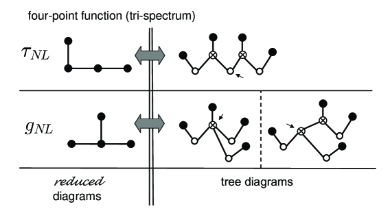
Figure 9: The diagrams for the tri-spectrum. As we have mentioned in the previous section II.2, for the tri-spectrum due to the difference of the scale dependence we need the two parameters $\tau_{NL}$ and $g_{NL}$, which can be also distinguished by using the reduced diagram. Using the tree diagram $g_{NL}$ is decomposed to two diagrams as shown in this figure. The arrows indicate the focused vertex in each diagram.

We choose a focused vertex in each diagram as indicated by arrows in Fig. 9. Following the prescription explained in the preceding section, we have

$$\tau_{NL}=W_{*}^{-3}\left[A^{ab}\Omega_{a}(N_{*})\Omega_{b}(N_{*})\right],$$ (IV.5)

$$g_{NL}={25\over 54}W_{*}^{-3}\Biggl{\{}N_{abc}^{F}\tilde{N}^{a}(N_{F})\tilde{N}^{b}(N_{F})\tilde{N}^{c}(N_{F})+\int^{N_{F}}_{N_{*}}dNN_{a}(N)Q^{a}_{(4)bcd}(N)\tilde{N}^{b}(N)\tilde{N}^{c}(N)\tilde{N}^{d}(N)~{}$$

$$\qquad\qquad\qquad\qquad\qquad+3\int^{N_{F}}_{N_{*}}dN\Omega_{a}(N)Q^{a}_{(3)bc}(N)\tilde{N}^{b}(N)\tilde{N}^{c}(N)\Biggl{\}}~{}.$$ (IV.6)

where $\Omega_{a}(N)$ is a new vector obtained by solving

$${d\over dN}\Omega_{a}(N)=-\Omega_{b}(N)P^{b}_{~{}a}(N)-N_{b}(N)Q^{b}_{(3)ac}(N)\tilde{N}^{c}(N)~{},$$ (IV.7)

backward in time from $N=N_{F}$ with the boundary conditions $\Omega_{a}(N_{F})=N_{ab}^{F}\tilde{N}^{b}(N_{F})$. The first (second) line on the right hand side of $g_{\rm NL}$ represents the contribution of the left (right) tree diagram corresponding to $g_{NL}$ in Fig. 9. In our formulation, it is enough to solve differential equations for three vectors $N_{a},~{}{\tilde{N}}^{a},~{}\Omega_{a}$ to compute $\tau_{\rm NL}$ and $g_{\rm NL}$.

IV.4 quad-spectrum

In order to demonstrate the efficiency of our formulation, we show the explicit formula for the quad-spectrum. We also show the correspondence between the reduced diagram and the tree diagram for the fifth-order spectrum (five-point correlation function) in Fig. 10.

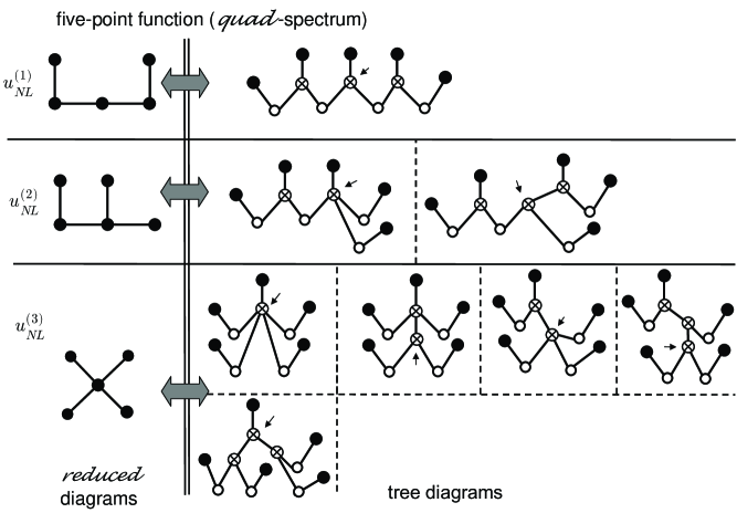
Figure 10: This shows the correspondence between reduced diagram and the tree diagram for the fifth-order spectrum as an example. The arrows indicate the focused vertex in each diagram.

Using the formula, we obtain an expression for the quad-spectrum as

$$\langle\zeta_{{\bf k}_{1}}\zeta_{{\bf k}_{2}}\zeta_{{\bf k}_{3}}\zeta_{{\bf k}_{4}}\zeta_{{\bf k}_{5}}\rangle_{c} = u^{(1)}_{NL}\left(P_{\zeta}(k_{1})P_{\zeta}(k_{12})P_{\zeta}(k_{45})P_{\zeta}(k_{5})+59~{}{\rm perms.}\right)$$ (IV.8)

$$+u^{(2)}_{NL}\left(P_{\zeta}(k_{1})P_{\zeta}(k_{12})P_{\zeta}(k_{4})P_{\zeta}(k_{5})+59~{}{\rm perms.}\right)$$

$$+u^{(3)}_{NL}\left(P_{\zeta}(k_{1})P_{\zeta}(k_{2})P_{\zeta}(k_{3})P_{\zeta}(k_{4})+4~{}{\rm perms.}\right),$$

with

$$u^{(1)}_{NL}=W_{*}^{-4}\Biggl{\{}\int^{N_{F}}_{N_{*}}dNN_{a}(N)\hat{Q}^{a}_{(3)bc}(N)\tilde{\Omega}^{b}(N)\tilde{\Omega}^{c}(N)\Biggr{\}}~{},$$ (IV.9)

$$u^{(2)}_{NL}=W_{*}^{-4}\int^{N_{F}}_{N_{*}}dN\Biggl{\{}N_{a}(N)\hat{Q}^{a}_{(4)bcd}(N)\tilde{\Omega}^{b}(N)\tilde{N}^{c}(N)\tilde{N}^{d}(N)+3\Omega_{a}(N)\hat{Q}^{a}_{(3)bcd}(N)\tilde{\Omega}^{b}(N)\tilde{N}^{c}(N)\Biggr{\}}~{},$$ (IV.10)

$$u^{(3)}_{NL}=W_{*}^{-4}\int^{N_{F}}_{N_{*}}dN\Biggl{\{}N_{a}(N)\hat{Q}^{a}_{(5)bcde}(N)\tilde{N}^{b}(N)\tilde{N}^{c}(N)\tilde{N}^{d}(N)\tilde{N}^{e}(N)+6\Phi_{a}(N)\hat{Q}^{a}_{(3)bc}(N)\tilde{N}^{b}(N)\tilde{N}^{c}(N)$$ (IV.11)

$$\qquad\qquad\quad\quad\quad\quad\quad\quad\quad+4\Omega_{a}(N)\hat{Q}^{a}_{(4)bcd}(N)\tilde{N}^{b}(N)\tilde{N}^{c}(N)\tilde{N}^{d}(N)+12\Psi_{a}(N)\hat{Q}^{a}_{(3)bc}(N)\tilde{N}^{b}(N)\tilde{N}^{c}(N)$$ (IV.12)

$$\qquad\qquad\quad\quad\quad\quad\quad\quad\quad\quad\quad+3N_{a}(N)\hat{Q}^{a}_{(3)bc}(N)\tilde{\Pi}^{b}(N)\tilde{\Pi}^{c}(N)\Biggr{\}}~{}.$$ (IV.13)

Here we introduced new vectors defined by the equations

$$\frac{d}{dN}\tilde{\Omega}^{a}(N)=P^{a}_{~{}b}(N)\tilde{\Omega}^{b}(N),$$ (IV.14)

$$\frac{d}{dN}\Phi_{a}(N)=-P^{b}_{~{}a}(N)\Phi_{b}(N)-N_{b}(N)Q^{b}_{(4)cda}(N){\tilde{N}}^{c}(N){\tilde{N}}^{d}(N),$$ (IV.15)

$$\frac{d}{dN}\Psi_{a}(N)=-P^{b}_{~{}a}(N)\Psi_{b}(N)-\Omega_{b}(N)Q^{b}_{(3)ca}(N){\tilde{N}}^{c}(N),$$ (IV.16)

$$\frac{d}{dN}\tilde{\Pi}^{a}(N)=P^{a}_{~{}b}(N)\tilde{\Pi}^{b}(N)+Q^{a}_{(3)bc}\tilde{N}^{b}(N)\tilde{N}^{c}(N),$$ (IV.17)

with the boundary conditions $\tilde{\Omega}^{a}(N_{*})=A^{ab}\Omega_{b}(N_{*})$, $\Phi_{a}(N_{F})=N_{abc}^{F}\tilde{N}^{b}(N_{F})\tilde{N}^{c}(N_{F})$, $\Psi_{a}(N_{F})=0$ and $\tilde{\Pi}^{a}(N_{*})=0$.

V Discussion and conclusion

The primordial non-Gaussianity has been focused on by many authors as a new probe of the inflation dynamics. The deviation from the Gaussian statistics affects not only the bi-spectrum of the primordial curvature perturbations but also the higher order correlation functions. In general, to describe the higher order correlation functions, we need more parameters and more complicated calculations. Instead of resorting to the direct calculations, we developed a diagrammatic method, which is useful in counting the number of necessary non-linearity parameters and computing the higher order correlation functions for non-Gaussianity of local type. We showed that the number of parameters to describe the $n$-point correlation function is equal to the number of reduced tree diagrams with $n$ vertices that are not isomorphic to each other. We also found that in the calculation of general $n$-point correlation function we have only to solve the vector quantities which follow the same linear perturbation equation for the background field or it’s dual Yokoyama:2007dw , but with a source term and different boundary conditions. Our formalism requires the number of operations proportional to ${\cal N}$ even for higher order correlation functions, in contrast to the naive expectation $\propto{\cal N}^{n}$, where ${\cal N}$ is the number of components of the inflaton field. It will be clear that our formulation is particularly powerful for the inflation models with many components of scalar field, including the models in which the slow-roll conditions are violated after the horizon crossing time.

In this paper, we assumed that the distribution of initial perturbations of the field $\{\delta\varphi_{*}^{a}\}$ is Gaussian. As a results, in the diagram the number of lines connected to the open circle, which corresponds to the contraction of $\delta\varphi_{*}^{a}$, is two. When we need to consider the effects of non-Gaussianity of $\delta\varphi_{*}^{a}$, we can easily extend our formalism by adding open circles with appropriate numbers of the attached lines. For example, it has been well known that the leading effect of non-Gaussianity in $\delta\varphi_{*}^{a}$ affects the three-point correlation function as Byrnes:2006vq ; Seery:2006vu ; Seery:2006js

$$\langle\zeta_{{\bf k}_{1}}\zeta_{{\bf k}_{2}}\zeta_{{\bf k}_{3}}\rangle\equiv\left[N_{a}^{*}N_{b}^{*}N_{c}^{*}B^{abc}(k_{1},k_{2},k_{3})+{6\over 5}f_{NL}^{G}\left(P_{\zeta}(k_{1})P_{\zeta}(k_{2})+2~{}{\rm perms.}\right)\right]\delta^{(3)}({\bf k}_{1}+{\bf k}_{2}+{\bf k}_{3})~{},$$ (V.1)

$$\langle\delta\varphi^{a}_{*}\delta\varphi^{b}_{*}\delta\varphi^{c}_{*}\rangle\equiv B^{abc}(k_{1},k_{2},k_{3})\delta^{(3)}({\bf k}_{1}+{\bf k}_{2}+{\bf k}_{3})~{},$$ (V.2)

where ${6\over 5}f_{NL}^{G}$ denotes the non-linearity parameter given by Eq. (IV.4), which has been obtained under the assumption that $\delta\varphi_{*}^{a}$ is Gaussian. In our diagrammatic method, the first term on the right hand side of Eq. (V.1) can be described by the diagram presented in Fig. 11. For this open circle $\circ$ with three legs we assign the factor $B^{abc}$ defined in (V.2). Generalization of taking into account the higher order correlators is straightforward. Application of our formulas to some explicit models will be reported in the forthcoming paper.

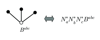
Figure 11: This diagram corresponds to the leading order correction due to the non-Gaussianity of the initial perturbation $\delta\varphi^{a}_{*}$ to the bi-spectrum.

Appendix A Proof of subsection II.2

We give a proof of the statement that the functions obtained by applying the rules in Sec. II.2 to two tree diagrams with $n$ vertices that are not isomorphic to each other show different wavenumber dependence Ota . To prove it, it is enough to show that we can uniquely reconstruct the tree diagram with $n$ vertices from a given function $f({\vec{k}_{1}},\cdots,{\vec{k}_{n}})$, which guarantees one-to-one correspondence between a diagram and a function $f({\vec{k}_{1}},\cdots,{\vec{k}_{n}})$. Here each wavenumber ${\vec{k}_{i}}$ is assigned to each vertex. By construction, the function $f$ should be a product of $(n-1)$ power spectra, $P$, whose arguments are the length of the sum of several wavenumbers taken from ${\vec{k}}_{i}(1\leq i\leq n)$.

Let us focus on one arbitrary vertex of the would-be reconstructed diagram. We refer to this vertex as $V_{m}$ and the vector attached to this vertex as ${\vec{k}}_{m}$. We eliminate ${\vec{k}}_{m}$ from the arguments of $P$ by using the relation ${\vec{k}}_{1}+\cdots+{\vec{k}}_{n}=0$. Then, the wavenumber assigned to a vertex connected to $V_{m}$ by a line must appear in $f$ only once. This is because such a wavenumber appears only in $P$ corresponding to the line that connects this vertex to $V_{m}$. By finding all such wavenumbers, we recognize all the vertices that are connected to the vertex $V_{m}$. By doing the same thing for each vertex, we completely recognize how all the vertices are mutually connected. Obviously, this fixes the shape of the diagram uniquely.

Appendix B Explicit formulas for derivatives of $N^{F}$

As mentioned in Sec. III.1, $N_{a_{1}a_{2\cdots}a_{n}}^{F}$ defined in Eq. (III.1) can be written in terms of local quantities evaluated at $N=N_{F}$. Here, as examples, we explicitly evaluate the coefficients $N_{a}^{F},N_{ab}^{F}$ and $N_{abc}^{F}$. Taking the hypersurface at $N=N_{F}$ to be a uniform Hubble one, which is equal to the uniform density slicing on super-horizon scales, we have the equation,

$$H\left(\varphi^{a}(N_{F}+\zeta(N_{F}))\right)=H\bigl{(}\!{\stackrel{{\,{}_{(0)}}}{{\varphi}}}\!^{a}(N_{F})\bigr{)}~{}.$$ (B.1)

The Hubble parameter $H$ is given by Eq. (II.5). In our previous paper Yokoyama:2007dw , solving Eq. (B.1) with respect to $\zeta(N_{F})$ up to the second order, we have obtained

$$N_{a}^{F}=-\frac{H_{a}(\varphi)}{H_{b}(\varphi)F^{b}(\varphi)}\biggr{|}_{\varphi=\!{\stackrel{{\,{}_{(0)}}}{{\varphi}}}\!(N_{F})}~{},$$ (B.2)

$$N_{ab}^{F}=-\frac{U_{ab}(\varphi)}{H_{c}(\varphi)F^{c}(\varphi)}\biggr{|}_{\varphi=\!{\stackrel{{\,{}_{(0)}}}{{\varphi}}}\!(N_{F})}~{},$$ (B.3)

where

$$U_{ab}=H_{ab}+2\left(H_{c}P^{c}_{~{}a}+F^{c}H_{ca}\right)N^{F}_{b}+\left(F^{c}H_{cd}F^{d}+H_{c}P^{c}_{~{}d}F^{d}\right)N_{a}^{F}N_{b}^{F}~{},$$ (B.4)

with $H_{a}\equiv\partial H/\partial\varphi^{a},~{}H_{ab}\equiv\partial^{2}H/\partial\varphi^{a}\partial\varphi^{b}$. Solving Eq. (B.1) up to the third order, we also obtain

$$N_{abc}^{F}=-{W_{abc}(\varphi)\over H_{d}(\varphi)F^{d}(\varphi)}\biggr{|}_{\varphi=\!{\stackrel{{\,{}_{(0)}}}{{\varphi}}}\!(N_{F})}~{},$$ (B.5)

where

$$W_{abc} \!=\! H_{abc}+\left[H_{d}\left(Q^{d}_{(3)ef}F^{e}+P^{d}_{~{}e}P^{e}_{~{}f}\right)F^{f}+H_{def}F^{d}F^{e}F^{f}+3F^{d}H_{de}P^{e}_{~{}f}F^{f}\right]N_{a}^{F}N_{b}^{F}N_{c}^{F}~{}$$ (B.6)

$$+3\left[2F^{d}H_{de}P^{e}_{~{}a}+\left(H_{ade}F^{d}+H_{ad}P^{d}_{~{}e}\right)F^{e}+H_{d}\left(Q^{d}_{(3)ea}F^{e}+P^{d}_{~{}e}P^{e}_{~{}a}\right)\right]N^{F}_{b}N^{F}_{c},~{}$$

$$+{3}\left(2H_{ad}P^{d}_{~{}b}+F^{d}H_{dab}+H_{d}Q^{d}_{(3)ab}\right)N_{c}^{F}~{}$$

$$+3\left(F^{d}H_{de}F^{e}+H_{d}P^{d}_{~{}e}F^{e}\right)N^{F}_{a}N^{F}_{bc}+3\left(F^{d}H_{da}+H_{d}P^{d}_{~{}a}\right)N^{F}_{bc}$$

with $H_{abc}\equiv{\partial^{3}H/\partial\varphi^{a}\partial\varphi^{b}\partial\varphi^{c}}$. Note that $U_{ab}$ and $W_{abc}$ are symmetric with respect to the indices. As we mentioned earlier, here we define the phase space variables as $\varphi^{I}_{1}=\phi^{I}$ and $\varphi^{I}_{2}=\dot{\phi}^{I}$.

References

- (1) E. Komatsu et al. [WMAP Collaboration], arXiv:0803.0547 [astro-ph].
- (2) E. Komatsu and D. N. Spergel, Phys. Rev. D 63, 063002 (2001) [arXiv:astro-ph/0005036].
- (3) N. Bartolo, E. Komatsu, S. Matarrese and A. Riotto, Phys. Rept. 402, 103 (2004) [arXiv:astro-ph/0406398].
- (4) T. Okamoto and W. Hu, Phys. Rev. D 66, 063008 (2002) [arXiv:astro-ph/0206155].
- (5) N. Bartolo, S. Matarrese and A. Riotto, JCAP 0508, 010 (2005) [arXiv:astro-ph/0506410].
- (6) N. Kogo and E. Komatsu, Phys. Rev. D 73, 083007 (2006) [arXiv:astro-ph/0602099].
- (7) G. D’Amico, N. Bartolo, S. Matarrese and A. Riotto, JCAP 0801, 005 (2008) [arXiv:0707.2894 [astro-ph]].
- (8) [Planck Collaboration], “Planck: The scientific programme,” arXiv:astro-ph/0604069.
- (9) C. T. Byrnes, K. Koyama, M. Sasaki and D. Wands, JCAP 0711, 027 (2007) [arXiv:0705.4096 [hep-th]].
- (10) S. Yokoyama, T. Suyama and T. Tanaka, JCAP 0707, 013 (2007) [arXiv:0705.3178 [astro-ph]].
- (11) S. Yokoyama, T. Suyama and T. Tanaka, Phys. Rev. D 77, 083511 (2008) [arXiv:0711.2920 [astro-ph]].
- (12) C. T. Byrnes, M. Sasaki and D. Wands, Phys. Rev. D 74, 123519 (2006) [arXiv:astro-ph/0611075].
- (13) A. A. Starobinsky, JETP Lett. 42, 152 (1985) [Pisma Zh. Eksp. Teor. Fiz. 42, 124 (1985)].
- (14) M. Sasaki and E. D. Stewart, Prog. Theor. Phys. 95, 71 (1996) [arXiv:astro-ph/9507001].
- (15) M. Sasaki and T. Tanaka, Prog. Theor. Phys. 99, 763 (1998) [arXiv:gr-qc/9801017].
- (16) D. H. Lyth, K. A. Malik and M. Sasaki, JCAP 0505, 004 (2005) [arXiv:astro-ph/0411220].
- (17) D. H. Lyth and Y. Rodriguez, Phys. Rev. Lett. 95, 121302 (2005) [arXiv:astro-ph/0504045].
- (18) H. R. S. Cogollo, Y. Rodriguez and C. A. Valenzuela-Toledo, JCAP 0808, 029 (2008) [arXiv:0806.1546 [astro-ph]].
- (19) D. Seery, J. E. Lidsey and M. S. Sloth, JCAP 0701, 027 (2007) [arXiv:astro-ph/0610210].
- (20) D. Seery and J. E. Lidsey, JCAP 0701, 008 (2007) [arXiv:astro-ph/0611034].
- (21) P. R. Jarnhus and M. S. Sloth, JCAP 0802, 013 (2008) [arXiv:0709.2708 [hep-th]].
- (22) F. Arroja and K. Koyama, Phys. Rev. D 77, 083517 (2008) [arXiv:0802.1167 [hep-th]].
- (23) The authors thank to Professor Katsuhiro Ohta at Keio University for providing the proof, private communication.
- (24) J. N. Fry, Astrophys. J. 279 (1984) 499.
- (25) J. Riorden, ”Introduction to Combinatorial Analysis”, Dover Publications, INC., Mineola, New York