CNO-driven winds of hot first stars

During the evolution of first stars, the CNO elements may emerge on their surfaces due to the mixing processes. Consequently, these stars may have winds driven purely by CNO elements. We study the properties of such stellar winds and discuss their influence on the surrounding environment. For this purpose, we used our own NLTE models and tested which stellar parameters of the first stars at different evolutionary stages result in CNO winds. If such winds are possible, we calculate their hydrodynamic structure and predict their parameters. We show that, while the studied stars do not have any wind driven purely by hydrogen and helium, CNO driven winds exist in more luminous stars. On the other hand, for very hot stars, CNO elements are too ionized to drive a wind. In most cases the derived mass-loss rate is much less than calculated with solar mixture of elements. This is because wind mass-loss rate in present hot stars is dominated by elements heavier than CNO. We conclude that, until a sufficient amount of these elements is created, the influence of line-driven winds is relatively small on the evolution of hot stars (which are not close to the Eddington limit).

1 Introduction

The only elements created in non negligible amounts during primordial nucleosynthesis are helium and hydrogen (e.g., Coc et al. 2004). Consequently, first stars, which formed from the pristine gas processed during this primordial nucleosynthesis, were pure hydrogen-helium stars. Numerical simulations of first star formation show that the primordial nucleosynthesis not only determined the chemical composition of these stars, but the absence of heavier elements also influenced the initial mass function of these stars (e.g., Bromm et al. 1999; Nakamura & Umemura 2002). In the absence of heavier elements, the only efficient cooling processes during the collapse of primordial haloes are those of molecular hydrogen. Since the molecular hydrogen line cooling is less efficient than, say cooling from dust, the temperature in the first star-forming regions was much higher than in the present-day star-forming regions. In the absence of fragmentation this led to very high masses of first stars (of the order of $10-100\,\text{M}_{\odot}$, Omukai & Palla 2003).

The general picture of the evolution of first stars is in many aspects different from the evolution of present hot stars (Marigo et al. 2001; Klapp et al. 2005; Hirschi 2007). One of the most important differences is the possible existence of pair-instability supernovae, which create a very typical pattern of nuclear yields (Heger & Woosley 2002). The possibility of creating a pair-instability supernova is closely connected to the total amount of mass lost by an individual star during its evolution. If the star does lose a significant fraction of the mass during its evolution, it may avoid the pair-instability supernova eruption (Ekström et al. 2007).

Current massive stars lose their mass via line-driven winds (see Kudritzki & Puls 2000; Krtička & Kubát 2007a, for reviews). These winds are accelerated mainly due to the absorption in the lines of heavier elements, such as iron, carbon, nitrogen, and oxygen. For these stars the amount of mass lost by the star per unit of time (the mass-loss rate) can be in principle derived both from observations and from theoretical modelling (e.g., Puls et al. 2006). However, given that there have not been any available observations of first stars up to now, we have to rely on the theoretical predictions alone in the case of first stars.

Stellar winds of pure hydrogen-helium extremely massive first stars were studied by Krtička & Kubát (2006, hereafter Paper II). We showed that the homogeneous line-driven winds of these stars are unlikely and that only an extremely weak pure hydrogen wind could be possible for stars very close to the Eddington limit. Stellar winds of very low-metallicity massive stars were studied by Kudritzki (2002) assuming the solar mixture of elements. On the basis of these models, Marigo et al. (2003) concludes that line-driven winds influence the evolution of non-rotating, very low-metallicity stars only negligibly. Stellar winds of stars at extremely low metallicity might be possible only if the star is very close to the Eddington limit (Kudritzki 2002; Vink & de Koter 2005; Gräfener & Hamann 2008).

During the core He-burning phase of first stars, primary nitrogen emerges on the stellar surface (Meynet et al. 2006; Hirschi 2007). This primary nitrogen is synthetised in the H-burning shell due to the rotational mixing of carbon and oxygen produced in the helium core. Moreover, evolutionary models of massive first stars (e.g., Meynet et al. 2006; Hirschi 2007) show that subsequent generation of stars could contain relatively large amounts of CNO elements, whereas the abundance of iron-peak elements was very low. This picture is also supported by observations of carbon-rich, extremely metal-poor stars (e.g., Norris et al. 1997).

However, the detailed study of stellar winds driven purely by CNO elements is still missing. Here we study such winds for the parameters typical of hot first stars.

2 Description of models

2.1 Basic assumptions

The models used in this paper are based on the NLTE wind models of Krtička & Kubát (2004, hereafter Paper I). Here we only summarise their basic features and describe improvements in atomic data.

We assume spherically symmetric stationary stellar wind. The excitation and ionization state of the considered elements is derived from the statistical equilibrium (NLTE) equations. For some ions we improved the atomic data and adopted the ionic models from the OSTAR2002 grid of model stellar atmospheres (Lanz & Hubeny 2003, 2007, see Table 1). These ionic models are based mainly on the Opacity Project data (Peach et al. 1988; Luo & Pradhan 1989; Tully et al. 1990; Seaton et al. 1992; Fernley et al. 1999). For some of these stars, the ionization fractions of some ions in the envelopes are so low that it is not meaningful to include these ions in the solution of the NLTE equations. The conditions for including such ions are also given in Table 1. The ionic list is modified in such a way that the highest considered ion is only included as its ground state.

Table 1: Atoms and ions included in the NLTE calculations.

Ion	Levels1	Data	Comment2
H i	9
H ii	1
He i	14		$T_{\text{eff}}<70\,000\,\text{K}$
He ii	14
He iii	1
C i	26		$T_{\text{eff}}<30\,000\,\text{K}$
C ii	14		$T_{\text{eff}}<35\,000\,\text{K}$
C iii	23	OSTAR20023	$T_{\text{eff}}<70\,000\,\text{K}$
C iv	25	OSTAR2002
C v	11
C vi	10		$T_{\text{eff}}>30\,000\,\text{K}$
C vii	1		$T_{\text{eff}}>50\,000\,\text{K}$
N i	21		$T_{\text{eff}}<30\,000\,\text{K}$
N ii	14		$T_{\text{eff}}<35\,000\,\text{K}$
N iii	32	OSTAR2002	$T_{\text{eff}}<70\,000\,\text{K}$
N iv	23	OSTAR2002
N v	16	OSTAR2002
N vi	15		$T_{\text{eff}}>20\,000\,\text{K}$
N vii	1		$T_{\text{eff}}>30\,000\,\text{K}$
O i	12		$T_{\text{eff}}<30\,000\,\text{K}$
O ii	50		$T_{\text{eff}}<35\,000\,\text{K}$
O iii	29	OSTAR2002	$T_{\text{eff}}<70\,000\,\text{K}$
O iv	39	OSTAR2002
O v	14
O vi	20	OSTAR2002	$T_{\text{eff}}>20\,000\,\text{K}$
O vii	1		$T_{\text{eff}}>30\,000\,\text{K}$

¹ An individual level or a set of levels merged into a superlevel.
² Note: the comment (if any) shows for which stars the individual ion is taken into an account. If the comment is missing, then the ion is considered for all models.
³ The ionic model taken from Lanz & Hubeny (2003).

As in Paper I, the radiative transfer problem is artificially split into two parts, namely the radiative transfer in continuum and the radiative transfer in lines. The solution of the radiative transfer equation in continuum is based on the Feautrier method in the spherical coordinates (Mihalas & Hummer 1974; Kubát 1993) with inclusion of all free-free and bound-free transitions of model ions, however neglecting line transitions.

The radiative transfer in lines is solved in the Sobolev approximation (Castor 1974) neglecting continuum opacity and line overlaps. The radiative force is calculated in the Sobolev approximation using data from the VALD database (Piskunov et al. 1995; Kupka et al. 1999). To test the completeness of our line list, we compared these data with the line-lists provided by the NIST database (Wiese et al. 1996) and given by Kurucz (1992) and enlarged the original data set when necessary. The radiative force due to the light scattering on free electrons is also included in the model calculations.

The surface emergent flux (i.e., the lower boundary condition for the radiative transfer in wind) is taken from H-He spherically symmetric NLTE model stellar atmospheres of Kubát (2003, and references therein).

Table 2: Radius $R_{*}$, mass $M$, and the effective temperature $T_{\text{eff}}$ of studied model stars

ZAMS stars					Evolved stars
Model	$R_{*}$	$M$	$T_{\text{eff}}$		Model	$R_{*}$	$M$	$T_{\text{eff}}$
	$[\text{R}_{\odot}]$	$[\text{M}_{\odot}$]	[kK]			$[\text{R}_{\odot}]$	$[\text{M}_{\odot}$]	[kK]
M999	4.23	100	94.4		M999-0	8.2	100	73.6
M700	3.44	70	89.5		M999-1	56.4	100	29.9
M500	2.82	50	84.1		M999-2	125	100	20.1
M300	2.10	30	74.0		M999-3	510	100	10.0
M200	1.65	20	65.3		M500-1	11.1	50	50.0
M150	1.48	15	57.3		M500-2	33.7	50	29.9
M120	1.42	12	49.9		M500-3	72.0	50	20.6
M100	1.37	10	44.5		M500-4	303	50	10.1
M090	1.34	9	41.6		M200-1	4.1	20	50.0
M080	1.31	8	38.5		M200-2	19.9	20	24.5
M070	1.30	7	34.8		M100-1	11.4	10	20.2
M060	1.27	6	31.4		M100-2	45.6	10	9.8
M050	1.23	5	27.7		M050-1	5.1	5	20.1
M040	1.17	4	23.6
M030	1.11	3	19.1
M020	1.00	2	13.7

Parameters of these stars (given in Table 2) were obtained according to the evolutionary calculations of initially zero-metallicity stars derived by Marigo et al. (2001). We selected stellar parameters corresponding to the zero-age main sequence of these models and to later evolutionary phases to cover a larger area of the HR diagram.

2.2 The wind tests

Since we do not know in advance whether the radiative force is strong enough for a given star and chemical composition to drive a wind, we first test whether a wind may even exist. For these tests (see also Paper II, ), the hydrodynamical variables (velocity, temperature, and the density) are kept fixed. This enables us to calculate the model occupation numbers and the radiative force even in the case when the wind does not exist. The comparison of calculated radiative force and the gravitational force serves as a test of whether the wind exists; i.e., the winds are only possible when the magnitude of the radiative acceleration $g^{\text{rad}}$ is greater than the magnitude of the gravity acceleration $g$,

$$g^{\text{rad}}>g.$$ (1)

Besides the cotribution of lines, we also include the radiative acceleration due to the bound-free and free-free transitions in the calculation of the total radiative acceleration $g^{\text{rad}}$.

The velocity structure of our models is given by an artificial velocity law (see the discussion in Paper II, )

$$v(r)=10^{-3}\sqrt{\frac{5}{3}\frac{kT_{\text{eff}}}{m_{\text{H}}}}+2\times 10^{8}\,\text{cm\,s}^{-1}\frac{r-R_{*}}{R_{*}},$$ (2)

where $T_{\text{eff}}$ is the stellar effective temperature, $R_{*}$ the stellar radius, and $m_{\text{H}}$ the mass of the hydrogen atom. The density structure is obtained from the equation of continuity. In these models we assume a constant wind temperature $0.8T_{\text{eff}}$, and the electron density is consistently calculated from the ionization balance. Since for these wind tests we do not solve the equation of motion, it is necessary to specify wind mass-loss rate for which the wind existence is tested. For each set of stellar parameters the wind existence is tested for mass-loss rates $10^{-8}\,\text{M}_{\odot}\,\text{year}^{-1}$, $10^{-10}\,\text{M}_{\odot}\,\text{year}^{-1}$, and $10^{-12}\,\text{M}_{\odot}\,\text{year}^{-1}$.

To obtain a correct surface flux we accounted for the Doppler effect during the calculation of radiative transfer in lines, i.e. we shifted the stellar surface flux according to the actual wind velocity (Babel 1996).

2.3 Hydrodynamic wind models

For those stars, for which the wind test showed that the wind is possible, we also calculated hydrodynamic wind models (described in Paper I, ). In these models we consistently solved the hydrodynamical equations, i.e. the continuity equation, the momentum equation, and the energy equation with radiative cooling and heating included using the electrons thermal balance method (Kubát et al. 1999).

These models enable us to derive the radial variations of wind density, velocity, temperature, and the occupation numbers of individual excitation states. They especially enable us to predict the wind mass-loss rate and the terminal velocity.

3 Pure H-He winds

In Paper II we showed that the extremely massive ($M\geq 100\,\text{M}_{\odot}$), hot, pure hydrogen-helium stars do not have any wind. Stars very close to the Eddington limit with $\Gamma\gtrsim 0.859$ might be the only exception to this, since these stars can have very weak pure hydrogen wind. The absence of winds is connected with the material in the vicinity of these stars beeing ionized and consequently the line transitions are not strong enough to drive a wind. On the other hand, the material in the envelopes of the cooler, less massive stars studied here may be less ionized, thus giving the possibility to drive a wind. Here we test whether studied stars may have winds driven purely by hydrogen and helium.

For very hot stars, with $T_{\mathrm{eff}}\gtrsim 5\cdot 10^{4}\,\text{K}$ both hydrogen and helium are completely ionized in the envelopes; consequently, the radiative force due to the line transitions of these elements is by three to four orders of magnitude lower than the absolute value of the gravitational force. The most significant contribution to the radiative force is caused by the light scattering on free electrons for these stars.

For cooler stars, helium may be partly singly ionized; however, these stars have very broad photospheric lines, making the flux at the line positions so low that it does not allow the wind to accelerate. For stars with $T_{\text{eff}}\lesssim 20\,000\,\text{K}$, helium may in addition become partly neutral (in the envelopes with highest densities). However, the flux in the ultraviolet part of the spectrum where the neutral helium resonance lines appear is so low that the radiative force due to these lines is too low to accelerate the wind. In all these envelopes the hydrogen is nearly completely ionized, so that the radiative force due to hydrogen lines is negligible.

4 Analytical models of CNO line-driven winds

Before discussing more detailed numerical NLTE wind models of CNO line-driven winds, we first provide simplified analytic models of these winds (c.f., Abbott 1980; Owocki 2004; Feldmeier & Shlosman 2002).

The radiative acceleration in the Sobolev approximation is the sum of the contributions by individual lines (Castor 1974)

$$g^{\text{rad}}=\frac{8\pi}{\rho c^{2}}\frac{v}{r}\sum_{\mathrm{lines}}\nu_{ij}H_{c}(\nu_{ij})\int_{\mu_{*}}^{1}\text{d}\mu\,\mu\left(1+\sigma\mu^{2}\right)\left(1-e^{-\tau_{\mu}}\right),$$ (3)

where $H_{c}(\nu_{ij})$ is the emergent flux from the stellar atmosphere at the frequency $\nu_{ij}$ of a given line, $v$ is the radial wind velocity, $\rho$ the wind density,

$$\sigma= \frac{r}{v}\frac{\text{d}v}{\text{d}r}-1,$$ (4)

$$\mu_{*}= \left(1-\frac{R_{*}^{2}}{r^{2}}\right)^{1/2},$$ (5)

and the Sobolev optical depth $\tau_{\mu}$ is given by (Castor 1974; Rybicki & Hummer 1978)

$$\tau_{\mu}=\frac{\pi e^{2}}{m_{\mathrm{e}}\nu_{ij}}\left(\frac{n_{i}}{g_{i}}-\frac{n_{j}}{g_{j}}\right)g_{i}f_{ij}\frac{r}{v\left(1+\sigma\mu^{2}\right)},$$ (6)

where $n_{i}$, $n_{j}$, $g_{i}$, $g_{j}$ are the number densities and the statistical weights of individual states giving rise to a given line with the oscillator strength $f_{ij}$.

4.1 Wind driven by optically thick lines

Generally, the stellar wind of present hot stars is driven by an ensemble of optically thick and thin lines, the optically thick lines being important due to their strength and the optically thin ones due to their large number (e.g., Puls et al. 2000). The situation in the winds driven purely by CNO elements is different. Contrary to say, iron, these elements do not have many lines to drive wind, and the optically thick lines become much more important. In many cases there are just few optically thick lines that drive a wind. In such cases (for $\tau_{\mu}\gtrsim 3$ to obtain a precision of $5\%$), the radiative acceleration Eq. (3) is given roughly by

$$g^{\text{rad}}_{\text{thick}}=\frac{4\pi vR_{*}^{2}}{\rho c^{2}r^{3}}\left[\frac{r}{v}\frac{\text{d}v}{\text{d}r}-\frac{1}{2}\left(\frac{r}{v}\frac{\text{d}v}{\text{d}r}-1\right)\frac{R_{*}^{2}}{r^{2}}\right]\sum_{\mathrm{thick}\atop\mathrm{lines}}\nu_{ij}H_{c}(\nu_{ij}).$$ (7)

The momentum equation neglecting the gas pressure term and introducing the Eddington parameter,

$$\Gamma=\frac{g_{\text{e}}^{\text{rad}}}{g}=\frac{1}{g}\frac{\sigma_{\text{e}}L}{4\pi cr^{2}},$$ (8)

takes the form

$$F(r,v,\frac{\text{d}v}{\text{d}r})=v\frac{\text{d}v}{\text{d}r}-g^{\text{rad}}_{\text{thick}}+\frac{(1-\Gamma)GM}{r^{2}}=0.$$ (9)

Here, $g_{\text{e}}^{\text{rad}}$ is the radiative acceleration due to the free electrons, $L$ the stellar luminosity, $\sigma_{\text{e}}={n_{\text{e}}s_{\text{e}}}/{\rho}$, $s_{\text{e}}$ the Thomson scattering cross-section, $n_{\mathrm{e}}$ the electron number density, and $g=GM/r^{2}$. The momentum equation (9) has the critical point defined by $\left.\partial F(r,v,\frac{\text{d}v}{\text{d}r})/\partial\left(\frac{\text{d}v}{\text{d}r}\right)\right|_{r_{\text{crit}}}=0$ ($r_{\text{crit}}$ is the critical point radius)

$$\dot{M}\equiv 4\pi r^{2}\rho v=\frac{16\pi^{2}R_{*}^{2}}{c^{2}}\left(1-\frac{1}{2}\frac{R_{*}^{2}}{r_{\text{crit}}^{2}}\right)\sum_{\mathrm{thick}\atop\mathrm{lines}}\nu_{ij}H_{c}(\nu_{ij}),$$ (10)

which yields the wind mass-loss rate. Contrary to the original analysis presented by Castor et al. (1975, hereafter CAK), the critical point condition is simpler, as the radiative force depends on the velocity gradient linearly here. It would be possible to use the regularity condition to derive $r_{\text{crit}}$ and $\dot{M}$ (as was done in CAK); however, as in most cases $r_{\text{crit}}\approx R_{*}$, the wind mass-loss rate can be roughly given by

$$\dot{M}\approx\frac{8\pi^{2}R_{*}^{2}}{c^{2}}\sum_{\mathrm{thick}\atop\mathrm{lines}}\nu_{ij}H_{c}(\nu_{ij}).$$ (11)

This equation states that the mass-loss rate of the wind driven purely by optically thick lines is approximately given by the photon mass-loss rate ($L/c^{2}$) multiplied by the number of thick lines (Lucy & Solomon 1970; Owocki 1994). It can be shown that Eq. (10) also defines the point where the wind velocity is equal to the speed of so-called Abbott waves (Abbott 1980; Feldmeier et al. 2008).

Using the mass-loss rate estimate Eq. (11) and the definition of the mass-loss rate ($\dot{M}=4\pi r^{2}\rho v$), the momentum equation Eq. (9) can be rewritten as

$$v\left(1-\frac{R_{*}^{2}}{r^{2}}\right)\frac{\text{d}v}{\text{d}r}=\frac{(1-\Gamma)GM}{r^{2}}-\frac{R_{*}^{2}v^{2}}{r^{3}}.$$ (12)

This equation has a critical point at $r_{\text{crit}}=R_{*}$. To ensure the finiteness of the velocity derivative at this point, the righthand side of Eq. (12) should be equal to zero. This yields the value of the wind velocity at the critical point

$$v_{\text{crit}}=\sqrt{\frac{(1-\Gamma)GM}{R_{*}}}.$$ (13)

The application of the l’Hôpital rule to the momentum equation Eq. (12) at the critical point (Lamers & Cassinelli 1999) gives the value of the velocity derivative at this point:

$$\frac{\text{d}v}{\text{d}r}=\frac{1}{4R_{*}}\sqrt{\frac{(1-\Gamma)GM}{R_{*}}}.$$ (14)

4.2 Theoretical limits for CNO line-driven winds

In an accelerating outflow, the radiative force and the thermal pressure have to overcome gravity and inertia at each point in wind. As the thermal pressure is only effective at the base of the wind, the necessary condition for launching line-driven stellar wind is that the magnitude of radiative force should exceed the magnitude of gravitational force at a certain point in the wind, Eq. (1). We apply this condition to derive the minimal mass-loss rate of homogeneous wind (i.e. composed of all constituents, namely hydrogen, helium, carbon, nitrogen, and oxygen).

For a given set of lines, the radiative force is maximum if the lines are not self-shadowed, i.e. if the lines are optically thin and the line optical depths $\tau<1$ (Gayley 1995). Thus, for given occupation numbers, the line acceleration Eq. (3) cannot be higher than (see also Paper II, Eq. (2))

$$g^{\text{rad, max}}=\frac{4\pi^{2}e^{2}}{\rho m_{\text{e}}c^{2}}\left(\frac{R_{*}}{r}\right)^{2}\sum_{\text{lines}}H_{c}(\nu_{ij})g_{i}f_{ij}\left(\frac{n_{i}}{g_{i}}-\frac{n_{j}}{g_{j}}\right).$$ (15)

The condition of the wind existence Eq. (1) then reads as (c.f. Kudritzki 2002)

$$g^{\text{rad, max}}+g_{\text{e}}^{\text{rad}}=\left(\bar{Q}+1\right)g_{\text{e}}^{\text{rad}}>g,$$ (16)

where the parameter $\bar{Q}\equiv g^{\text{rad, max}}/g_{\text{e}}^{\text{rad}}$ was introduced by Gayley (1995). Neglecting the term with the number density of the upper level in Eq. (15) (which means neglecting stimulated emission) and substituting $g=GM/r^{2}$, the wind condition (16) can be rewritten as

$$\frac{4\pi^{2}e^{2}R_{*}^{2}}{\rho m_{\text{e}}c^{2}G{M}}\sum_{\text{lines}}H_{c}(\nu_{ij})f_{ij}n_{i}+\Gamma>1.$$ (17)

For a very low density of CNO elements, only the strongest lines (i.e., the resonance lines of the most abundant ions) significantly contribute to the radiative force (e.g., Krtička et al. 2006). In such a case, condition (17) can be rewritten as

$$\frac{4\pi^{2}e^{2}R_{*}^{2}}{m_{\text{e}}c^{2}G{M}}\sum_{\text{res}}H_{c}(\nu_{ij})f_{ij}\frac{Z_{\text{el}}}{m_{\text{el}}}+\Gamma>1,$$ (18)

where $Z_{\text{el}}$ is the mass fraction of element corresponding to the transition $i\leftrightarrow j$ (the ratio of the element density to the wind density), $m_{\text{el}}$ is the element mass, and the summation goes over the resonance lines of only the most abundant ions. If there is only one such element, then the minimum mass fraction of this element needed to drive the wind is given by

$$Z_{\text{el}}=\frac{m_{\text{e}}m_{\text{el}}c^{2}G{M}}{4\pi^{2}e^{2}R_{*}^{2}}\left(1-\Gamma\right)\left(\sum_{\text{res}}H_{c}(\nu_{ij})f_{ij}\right)^{-1}.$$ (19)

In scaled quantities, Eq. (19) takes the form of

$$Z_{\text{el}}=0.04A_{\text{el}}\left(1-\Gamma\right)\left(\frac{M}{1\,\text{M}_{\odot}}\right)\left(\frac{R_{*}}{1\,\text{R}_{\odot}}\right)^{-2}\times\\ \left[\sum_{\text{res}}\left(\frac{H_{c}(\nu_{ij})}{10^{-7}\,\text{erg}\,\text{cm}^{-2}}\right)f_{ij}\right]^{-1},$$ (20)

where $A_{\text{el}}$ is the elemental mass in units of hydrogen mass. Consequently, the minimum metallicity necessary for driving a wind depends on the surface gravity $g=GM/R_{*}^{2}$, and on the stellar effective temperature that determines both the ionization balance and the radiation flux.

The minimum mass-loss rate that can be driven from the star is given by the condition that at least one line remains to be optically thick at the critical point, i.e. $\tau_{\mu}>1$, where $\tau_{\mu}$ is given by Eq. (6). Using Eqs. (13) and (14), we can show (assuming $r_{\text{crit}}\approx R_{*}$ and for radial rays $\mu=1$) that the mass-loss rate should fulfil the condition

$$\dot{M}>\frac{m_{\text{el}}m_{\text{e}}}{e^{2}}\frac{\nu_{ij}(1-\Gamma)GM}{f_{ij}Z_{\text{el}}}.$$ (21)

For a typical case where there is only one optically thick line left, it can be readily shown (using the mass-loss rate estimate Eq. (11)) that the condition Eq. (21)

$$\frac{8\pi^{2}e^{2}R_{*}^{2}Z_{\text{el}}}{m_{\text{e}}m_{\text{el}}c^{2}G{M}}H_{c}(\nu_{ij})f_{ij}+\Gamma>1,$$ (22)

is nearly the same as the condition Eq. (18) written for one line. Consequently, if there is a line capable of overcoming the gravity (according to Eq. (18)), it is automatically optically thick one, and this line sets the mass-loss rate (and vice versa). In other words, for very low-density winds the condition of maximum radiative force Eq. (16) and the critical point analysis Sect. 4.1 give the same results for the existence of the wind and the wind’s mass-loss rate.

5 CNO-driven wind models

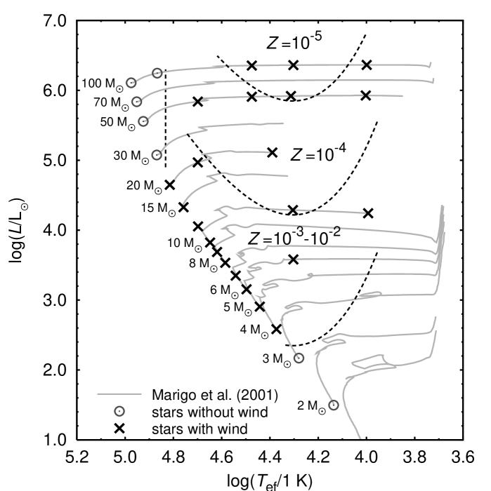
Figure 1: The HR diagram with minimal metallicity needed to drive a wind. Stars for which the winds are possible (for a studied range of metallicities) are denoted by crosses, and stars for which the winds are not possible are denoted by circles. The dashed lines denote boundaries separating stars with a different minimum metallicity necessary for driving a wind. The boundaries were derived using Eq. (18) and the Wien law. Overplotted are the evolutionary tracks of Marigo et al. (2001).

For the parameters of model stars given in Table 2, we tested whether these stars could have CNO driven winds. We tested the possibility of the wind for the mass-loss rates $10^{-12}\,\text{M}_{\odot}\,\text{year}^{-1}$, $10^{-10}\,\text{M}_{\odot}\,\text{year}^{-1}$, and $10^{-8}\,\text{M}_{\odot}\,\text{year}^{-1}$, and for the mass fraction of CNO elements in the range of $10^{-4}-0.1$ with a relative step of 10. We assumed the same number density for carbon, nitrogen, and oxygen.

The regions in the HR diagram corresponding to the parameters of stars for which the wind tests are positive are given in Fig. 1. The minimum mass fraction of CNO needed to drive the wind is also indicated there.

For parameters for which the wind may exist, we calculated hydrodynamic wind models and predicted the mass-loss rate (again assuming the same number density of CNO). Calculated wind parameters for individual stars are given in Appendix in Table A. The mass-loss rate of studied stars can be fitted by the formula

$$\dot{M}(L,Z,T_{\text{eff}})=\alpha_{0}\,L^{\alpha_{1}}\,10^{\textstyle\frac{\alpha_{2}\left(\log Z+\alpha_{3}\log L\right)}{\log Z(\alpha_{4}+\alpha_{5}\log L)+1}\scriptstyle+\alpha_{6}\log T_{\text{eff}}},$$ (23)

where the luminosity $L$ is expressed in the solar luminosity units $\text{L}_{\odot}$, $Z$ is the mass fraction of heavier elements, and $T_{\text{eff}}$ is expressed in the units of Kelvin. The values of parameters $\alpha_{0},\dots,\alpha_{6}$ fitted using the subroutine VARPRO (Golub & Pereyra 1973; Bolstad 1977) for the stellar groups with different effective temperatures are given in Table 3. For $\log Z(\alpha_{4}+\alpha_{5}\log L)+1<0$ the predicted mass-loss rate is set to zero.

In present-day hot stars, the modified wind momentum $\dot{M}{v}_{\infty}\left(R/\text{R}_{\sun}\right)^{1/2}$ depends mainly on the stellar luminosity (Kudritzki & Puls 2000, and references therein). According to its value, these stars can be divided into four groups (see Fig. 2).

Figure 2: The modified wind momentum-luminosity relationship for stars with different effective temperatures and $Z=0.01$. Stars with $T_{\text{eff}}\gtrsim 70\,000\,\text{K}$ do not have any wind. Overplotted is the mean dependence of the modified wind momentum predicted for O stars with solar metallicity by Krtička & Kubát (2007b).

Table 3: The best-fit parameters of Eq. (23) for individual stellar groups

$T_{\text{eff}}$ [K]	$\alpha_{0}$ [$\text{M}_{\odot}\,\text{year}^{-1}$]	$\alpha_{1}$	$\alpha_{2}$	$\alpha_{3}$	$\alpha_{4}$	$\alpha_{5}$	$\alpha_{6}$
$<28\,000$	$1.19\times 10^{-23}$	$0.8437$	$0.2936$	$0.7167$	$0.1208$	$0.0064$	$2.4369$
$28\,000-40\,000$	$8.92\times 10^{-11}$	$0.7895$	$0.6123$	$0.8181$	$0.2848$	$-0.020158$	$-0.7394$
$>40\,000$	$2.39\times 10^{11}$	$0.5722$	$0.8348$	$0.7995$	$0.3983$	$-0.03542$	$-5.363$

5.1 Stars with no wind: $T_{\text{eff}}\gtrsim 70\,000\,\text{K}$

For the hottest stars with the effective temperature $T_{\text{eff}}\gtrsim 70\,000\,\text{K}$, we did not find that the wind exists. Although these stars are very luminous, their envelope is highly ionized with ions vi– vii being the dominant ionization states of CNO elements. Since the factor $\left({M}/{1\,\text{M}_{\odot}}\right)\left({R_{*}}/{1\,\text{R}_{\odot}}\right)^{-2}$ in Eq. (20) is larger than one for all these stars, a strong flux at the line position is needed to accelerate the wind. However, ions vi– vii have strong resonance lines in the far UV region (for frequencies higher than the He ii ionization threshold), where very low flux is emitted, so we do not find any wind for these stars.

5.2 Hottest stars with winds: $40\,000\,\text{K}\lesssim T_{\text{eff}}\lesssim 70\,000\,\text{K}$

Stars with the effective temperatures in the range $40\,000\,\text{K}\lesssim T_{\text{eff}}\lesssim 70\,000\,\text{K}$ may have a line-driven wind accelerated mainly by the O v and O vi lines. The hydrogen-like ion C vi and the helium-like one N vi, which are dominant ionization fractions of carbon and nitrogen, do not contribute significantly to the radiative force. The latter ions do not have enough strong resonance lines at the wavelengths at which strong flux is emitted. The minimum mass fraction of CNO elements needed to drive a wind agrees with analytical estimate Eq. (20) and is relatively high, of the order of $10^{-3}$ for ZAMS stars and as low as $10^{-4}$ for more evolved stars with larger radii.

The winds of hottest stars in this sample are accelerated mainly by the O vi resonance doublet 2s $\@element[\text{e}][2]{\mathrm{S}}$ $\rightarrow$ 2p $\@element[\text{o}][2]{\mathrm{P}}$. The analytic formula Eq. (11) gives the asymptotic value of the mass-loss rate if both lines of the doublet are optically thick (i.e., for high metallicity), while for lower metallicity the lines become optically thinner and the mass-loss rate decreases. For example, for the model star M150, the agreement between the mass-loss rate given by Eq. (11) $7.5\times 10^{-10}\,\text{M}_{\odot}\,\text{year}^{-1}$ and the mass-loss rate $6.4\times 10^{-10}\,\text{M}_{\odot}\,\text{year}^{-1}$ predicted for $Z=0.02$ by our hydrodynamic wind models shows a reliability of Eq. (11).

The winds of ZAMS stars are very weak (with the mass-loss rate of the order of $10^{-10}\,\text{M}_{\odot}\,\text{year}^{-1}$ for the solar chemical composition) due to their relatively low luminosity, whereas the winds of supergiants may be stronger with the mass-loss close to $10^{-7}\,\text{M}_{\odot}\,\text{year}^{-1}$.

For these stars the fitting formula Eq. (23) only gives reliable predictions for $\dot{M}\gtrsim 10^{-9}\,\text{M}_{\odot}\,\text{year}^{-1}$, for winds with smaller $\dot{M}$ the error could be of a factor of 3.

5.3 Stars with $28\,000\,\text{K}\lesssim T_{\text{eff}}\lesssim 40\,000\,\text{K}$

For stars $28\,000\,\text{K}\lesssim T_{\text{eff}}\lesssim 40\,000\,\text{K}$, the wind is possible, and carbon and nitrogen become more important for the driving of the wind, especially for cooler stars. The metallicity needed to drive a wind is about $10^{-4}-10^{-3}$ for ZAMS stars and may be extremely low ($\sim 10^{-5}$) for most massive evolved stars. This is connected with the relatively large factor $\left({M}/{1\,\text{M}_{\odot}}\right)\left({R_{*}}/{1\,\text{R}_{\odot}}\right)^{-2}$ in Eq. (20) for ZAMS stars (these stars are relatively compact), whereas this factor is lower for massive evolved stars with large radii.

5.4 The coolest stars with $10\,000\,\text{K}\lesssim T_{\text{eff}}\lesssim 28\,000\,\text{K}$

The coolest ZAMS stars with $T_{\text{eff}}\lesssim 20\,000\,\text{K}$ do not have any wind because these stars have a too high surface gravity to accelerate the wind. On the other hand, evolved massive stars may have winds even for metallicities as low as $10^{-5}$. For $Z\approx 0.01$, Pop III supergiant winds may have relatively high mass-loss rates of about $10^{-6}\,\text{M}_{\odot}\,\text{year}^{-1}$, comparable to present-day hot star winds. The winds of these stars are mainly accelerated by singly and doubly ionized carbon and nitrogen. Oxygen does not contribute significantly to the radiative force in this temperature range as the resonance lines of singly and doubly ionized oxygen have higher frequencies than the hydrogen ionization frequency, and only a relatively weak radiative flux is emitted there.

For the coolest stars, the fitting formula Eq. (23) can only be used for higher mass-loss rates $\dot{M}\gtrsim 10^{-9}\,\text{M}_{\odot}\,\text{year}^{-1}$.

6 Consequences of the wind’s existence

6.1 Influence on the stellar evolution

Our results show that the winds of first stars driven by CNO elements are rather weak compared to the winds of present-day hot stars. This is caused by two effects, the smaller number of CNO lines compared to, e.g., iron ones, and by the large surface gravity of first stars. Consequently, the estimated total mass lost due to winds during the stellar evolution is rather small. For example, assuming that the final abundance of CNO elements is a solar one, the estimate of the total mass loss of a star with an initial mass $M_{0}=100\,\text{M}_{\odot}$ is arround $1\,\text{M}_{\odot}$, and that of a star with $M_{0}=20\,\text{M}_{\odot}$ is about $0.1\,\text{M}_{\odot}$. Consequently, such stars lose only up to a few percent of their mass via line-driven winds.

In reality, the total mass lost might be even lower because CNO elements may occur at the stellar surface only in the later phases of the stellar evolution and the surface metallicity might be lower than the solar one.

6.2 Metal enrichment of the primordial halos

The presence of a relatively small amount of metals (with $Z\approx 10^{-5}-10^{-4}$) in the primordial haloes might inhibit subsequent formation of supermassive stars (see Loeb et al. 2008, for a review). Consequently, if the stellar winds of massive stars are strong enough, they can change the initial mass function in the primordial haloes.

If in the halo with the baryonic mass of about $10^{5}\,\text{M}_{\odot}$ a first star forms with the mass of $100\,\text{M}_{\odot}$, it might lose mass arround $1\,\text{M}_{\odot}$ due to the line-driven winds. Consequently, roughly $10^{-2}\,\text{M}_{\odot}$ of freshly synthesized CNO elements occur in such a halo, leading to the mass fraction of heavier elements of about $10^{-7}$, which is too low to change the initial mass function. The metallicity of the primordial halo would be enhanced more significantly only after the considered star explodes as a supernova.

7 Discussion

7.1 The chemical composition

The mass-loss rate predictions were calculated for the same number density of each of the CNO elements. In reality, the fraction of these elements is not uniform as assumed here. In such a case an approximate estimate of the wind mass-loss rate can be obtained as for different temperatures the wind is accelerated by different elements. For the hottest stars with $T_{\text{eff}}\gtrsim 40\,000\,\text{K}$, the wind is accelerated mainly due to oxygen lines (as supported by our models driven purely by oxygen), consequently for these stars the mass-loss rate depends mainly on the oxygen abundance. For cooler stars the wind is accelerated because of both carbon and nitrogen, so it could be roughly assumed that the wind mass-loss rate scales either with carbon or nitrogen abundance.

Stellar winds of present luminuous hot stars are mainly accelerated thanks to numerous heavier element lines (especially of iron and also of, e.g., nickel or copper, e.g., Pauldrach 1987; Puls et al. 2000; Vink et al. 2001) in the region where the wind mass-loss rate is determined, i.e. below the wind critical point. CNO elements do not have many strong lines available to drive a wind as do heavier elements. In the formalism of line-strength distribution functions, CNO elements and iron-peak elements dominate in different parts of the line-strength distribution function (Puls et al. 2000). As the result of this, CNO elements in present hot stars are important in the case when their large abundance (compared to iron-peak elements) enables their lines to continue beeing optically thick, i.e., in the outer wind regions of luminuous stars or in the weak winds of less luminuous stars (e.g., Vink et al. 2001; Krtička 2006; Krtička et al. 2006). These trends are reflected in the CNO mass-loss rate predictions presented here. Presented mass-loss rate predictions of luminuous stars are significantly lower than those derived assuming solar mixture of heavier elements (e.g., Vink et al. 2001; Kudritzki 2002; Krtička & Kubát 2004; Gräfener & Hamann 2005). On the other hand, the pure CNO mass-loss rate of less luminuous stars (or stars with very low metallicity) corresponds roughly to what is calculated assuming solar mixture of elements.

7.2 Comparison with literature

Since the wind models driven purely by CNO elements were not, to our knowledge, calculated for the studied stars, a direct comparison between our results and the results available in the literature is not possible. Pure CNO wind models were calculated by Unglaub (2008), but for different stellar parameters. However, at a very low wind density, the stellar winds are accelerated mostly by CNO lines and the contribution of heavier elements is basically negligible (e.g., Vink et al. 2001; Krtička et al. 2006). Consequently, an indirect comparison between our predictions and the predictions available in the literature for the lowest metallicities is feasible.

Kudritzki (2002) provided mass-loss rate predictions for very massive O stars at very low metallicities. The selected stellar sample overlaps with ours for the stars with mass $100\,\text{M}_{\odot}$. For these stars the lowest metallicities for which Kudritzki (2002) provides the mass-loss rate predictions reasonably agree with our minimum values of the metallicity needed to drive a wind (see Fig. 1). There is also reasonable agreement between our models and the models with the lowest mass-loss rate calculated by Vink et al. (2001) and Vink & de Koter (2005).

7.3 Multicomponent effects and pure metallic wind

The hydrogen and helium components of the stellar wind are accelerated mainly because of the collisions of hydrogen and helium atoms with heavier elements. Consequently, stellar winds of hot stars have a multicomponent nature (e.g., Owocki & Puls 2002; Krtička 2006). For low-density winds the transfer of momentum between radiationally accelerated metals and hydrogen and helium becomes inefficient. In this case the frictional heating or the decoupling of wind components may influence the wind structure.

If the decoupling occurs for velocities that exceed the escape speed, then the multicomponent effects do not influence the mass-loss rate (e.g., Votruba et al. 2007). On the other hand, if the decoupling occurs close to the star or in the stellar atmosphere, then the existence of pulsating shells (Porter & Skouza 1999) or pure metallic wind (Babel 1996) is possible.

Following Krtička (2006), we calculated the nondimensional velocity difference $x_{h\text{p}}$ between a given heavier element $h$ and the hydrogen-helium component. For small velocity differences $x_{h\text{p}}\lesssim 0.1$, the wind is well-coupled and can be modelled as a one-component one. For larger velocity differences $0.1\lesssim x_{h\text{p}}\lesssim 1$, the frictional heating influences the wind temperature, and for large velocity differences $x_{h\text{p}}\gtrsim 1$, the wind components decouple. The tests showed that, for nearly all wind models of ZAMS stars and for the low metallicity models of evolved stars, the multicomponent effects are indeed important. However, in most cases the multicomponent effects start to be important in the outer wind regions, so these effects do not affect the wind mass-loss rate.

For the cases when homogeneous wind is not possible, a pure metallic wind may exist (Babel 1996). We postpone the study of such stellar winds to a separate paper.

7.4 Model simplifications

The radiative force in the models presented here is calculated neglecting line overlaps and the influence of the line transitions on the continuum radiative transfer (see Krtička & Kubát 2004, for a more detailed discussion of the simplification of our code). However, these effects do not significantly influence the results here. First, CNO elements do not have as many lines as iron-peak elements; consequently, the line overlaps in CNO winds do not play as significant role as in the winds driven also by heavier elements. Second, the calculated mass-loss rate is relatively low, so the number of strong optically thick lines is relatively even lower. Finally, even for the winds driven by the solar mixture of elements our models are able to predict reliable wind parameters.

Hot star winds display small-scale inhomogeneities (clumping) that may influence the predicted wind mass-loss rate (e.g., de Koter et al. 2008). As the effect of these inhomogeneities on the wind mass-loss rate is not yet known, we neglect this effect.

7.5 H-He winds and other ways how to lose mass

A question might appear as to why the stellar wind driven purely by hydrogen and helium lines is not possible. This question is even more appealing in view of the fact that, in some models, the radiative force due to hydrogen may contribute a few percent to the total radiative force. To obtain a wind, in such a case, one would have to decrease the wind density. However, as the neutral hydrogen originates from the recombination, the decrease in the wind density leads to the decrease in the neutral hydrogen fraction and, consequently, to the decrease in the radiative force due to hydrogen. Consequently, as a result of this coupling the winds driven purely by hydrogen are not possible. A similar effects also occur for helium.

We note that there are several other possibilities how massive stars can lose their mass, although these possibilities were not up to now studied in greater detail. Stars with the luminosity higher than the corresponding Eddington limit may lose mass due to porous winds (Owocki et al. 2004) or via $\eta$ Car type of explosions (Smith & Owocki 2006). Moreover, stars rotating with the critical rotation rate may lose their mass via equatorial disc (e.g., Meynet et al. 2006).

8 Conclusions

We have studied the stellar winds of massive first stars to show that pure hydrogen-helium, hot first stars do not have any stellar wind. Only stars very close to the Eddington limit may have very weak pure hydrogen wind (Paper II).

As soon as CNO elements are synthesized in the stellar core and transported to the surface via the mixing processes, the CNO driven wind may exist for stars that fulfil the wind condition Eq. (18). We calculated the models for this wind and provided an approximate formula for calculating the mass-loss rate as a function of stellar parameters.

With decreasing $Z$, both the mass-loss rate and the number of optically thick lines decrease. We have shown that the condition that at least one line is optically thick Eq. (22) is nearly the same as the wind condition, Eq. (18) according to which the radiative force should be greater than gravity. Consequently, the wind ceases to exist for decreasing $Z$ both because the radiative force is too low and because all lines become optically thin.

We discussed the influence of CNO driven stellar winds on the stellar evolution and circumstellar environment. As the CNO elements are not able to accelerate the wind as efficiently as heavier elements, the wind mass-loss rates of CNO winds are relatively low. Consequently, the CNO winds do not significantly influence the stellar evolution or the circumstellar and interstellar environments.

We conclude that line-driven winds strong enough to influence the evolution of stars far away from the Eddington limit did not occur before the first supernova explosions.

Appendix A The derived wind parameters

Table 4: The wind parameters of studied stars calculated using hydrodynamic models

Model	$Z$	$\dot{M}$	$v_{\infty}$
		[$\text{M}_{\odot}\,\text{year}^{-1}$]	[$\text{km}\,\text{s}^{-1}$]
M040	$1\times 10^{-2}$	$2.9\times 10^{-12}$	$950$
M040	$2\times 10^{-2}$	$1.2\times 10^{-11}$	$1520$
M050	$3\times 10^{-3}$	$1.4\times 10^{-11}$	$1010$
M050	$5\times 10^{-3}$	$3.5\times 10^{-11}$	$1430$
M050	$1\times 10^{-2}$	$7.1\times 10^{-11}$	$2120$
M050	$2\times 10^{-2}$	$6.7\times 10^{-11}$	$3220$
M050-1	$1\times 10^{-3}$	$1.3\times 10^{-10}$	$1100$
M050-1	$3\times 10^{-3}$	$2.9\times 10^{-10}$	$1570$
M050-1	$1\times 10^{-2}$	$7.2\times 10^{-10}$	$1220$
M050-1	$2\times 10^{-2}$	$1.2\times 10^{-09}$	$830$
M060	$3\times 10^{-3}$	$1.8\times 10^{-11}$	$1630$
M060	$5\times 10^{-3}$	$3.5\times 10^{-11}$	$2260$
M060	$1\times 10^{-2}$	$5.8\times 10^{-11}$	$3240$
M060	$2\times 10^{-2}$	$7.9\times 10^{-11}$	$4470$
M070	$5\times 10^{-3}$	$3.4\times 10^{-11}$	$2360$
M070	$1\times 10^{-2}$	$1.1\times 10^{-10}$	$3410$
M070	$2\times 10^{-2}$	$2.0\times 10^{-10}$	$4310$
M080	$3\times 10^{-3}$	$6.7\times 10^{-11}$	$2440$
M080	$5\times 10^{-3}$	$1.3\times 10^{-10}$	$3250$
M080	$1\times 10^{-2}$	$2.1\times 10^{-10}$	$4540$
M080	$2\times 10^{-2}$	$3.3\times 10^{-10}$	$5950$
M090	$5\times 10^{-3}$	$3.0\times 10^{-11}$	$3010$
M090	$1\times 10^{-2}$	$9.1\times 10^{-11}$	$3500$
M090	$2\times 10^{-2}$	$3.5\times 10^{-10}$	$4790$
M100	$3\times 10^{-3}$	$3.7\times 10^{-11}$	$2540$
M100	$5\times 10^{-3}$	$7.3\times 10^{-11}$	$3320$
M100	$1\times 10^{-2}$	$2.7\times 10^{-10}$	$3340$
M100	$2\times 10^{-2}$	$6.0\times 10^{-10}$	$3790$
M100-1	$1\times 10^{-4}$	$9.1\times 10^{-11}$	$420$
M100-1	$3\times 10^{-4}$	$5.4\times 10^{-10}$	$930$
M100-1	$1\times 10^{-3}$	$1.3\times 10^{-09}$	$1530$
M100-1	$3\times 10^{-3}$	$3.3\times 10^{-09}$	$1030$
M100-1	$1\times 10^{-2}$	$6.3\times 10^{-09}$	$870$
M100-1	$2\times 10^{-2}$	$7.5\times 10^{-09}$	$1330$
M100-2	$1\times 10^{-2}$	$8.1\times 10^{-10}$	$800$
M100-2	$2\times 10^{-2}$	$1.0\times 10^{-09}$	$1070$
M120	$1\times 10^{-3}$	$6.9\times 10^{-12}$	$1020$
M120	$2\times 10^{-3}$	$1.2\times 10^{-10}$	$2050$
M120	$3\times 10^{-3}$	$2.1\times 10^{-10}$	$2540$
M120	$5\times 10^{-3}$	$3.5\times 10^{-10}$	$3630$
M120	$1\times 10^{-2}$	$4.9\times 10^{-10}$	$5130$
M120	$2\times 10^{-2}$	$6.1\times 10^{-10}$	$7110$
M150	$1\times 10^{-3}$	$1.6\times 10^{-11}$	$1420$
M150	$2\times 10^{-3}$	$1.6\times 10^{-10}$	$2700$
M150	$3\times 10^{-3}$	$2.8\times 10^{-10}$	$3370$
M150	$5\times 10^{-3}$	$4.2\times 10^{-10}$	$4350$
M150	$1\times 10^{-2}$	$5.7\times 10^{-10}$	$5950$
M150	$2\times 10^{-2}$	$6.4\times 10^{-10}$	$8110$
M200	$3\times 10^{-3}$	$3.8\times 10^{-10}$	$3120$
M200	$5\times 10^{-3}$	$5.7\times 10^{-10}$	$4200$
M200	$1\times 10^{-2}$	$7.7\times 10^{-10}$	$5840$
M200	$2\times 10^{-2}$	$9.1\times 10^{-10}$	$7680$
M200-1	$3\times 10^{-4}$	$6.7\times 10^{-10}$	$1470$
M200-1	$1\times 10^{-3}$	$3.0\times 10^{-09}$	$2800$
M200-1	$3\times 10^{-3}$	$5.6\times 10^{-09}$	$4020$
M200-1	$1\times 10^{-2}$	$9.4\times 10^{-09}$	$5630$
M200-1	$2\times 10^{-2}$	$1.3\times 10^{-08}$	$5130$

Model	$Z$	$\dot{M}$	$v_{\infty}$
		[$\text{M}_{\odot}\,\text{year}^{-1}$]	[$\text{km}\,\text{s}^{-1}$]
M200-2	$1\times 10^{-4}$	$7.0\times 10^{-09}$	$1000$
M200-2	$3\times 10^{-4}$	$2.0\times 10^{-08}$	$660$
M200-2	$1\times 10^{-3}$	$4.2\times 10^{-08}$	$780$
M200-2	$3\times 10^{-3}$	$5.5\times 10^{-08}$	$1490$
M200-2	$1\times 10^{-2}$	$6.4\times 10^{-08}$	$2650$
M200-2	$2\times 10^{-2}$	$6.9\times 10^{-08}$	$3360$
M500-1	$1\times 10^{-4}$	$8.3\times 10^{-09}$	$1510$
M500-1	$3\times 10^{-4}$	$2.7\times 10^{-08}$	$2440$
M500-1	$1\times 10^{-3}$	$6.3\times 10^{-08}$	$2750$
M500-1	$3\times 10^{-3}$	$9.9\times 10^{-08}$	$3460$
M500-1	$1\times 10^{-2}$	$1.3\times 10^{-07}$	$4060$
M500-1	$2\times 10^{-2}$	$1.6\times 10^{-07}$	$4680$
M500-2	$1\times 10^{-4}$	$7.6\times 10^{-08}$	$1010$
M500-2	$3\times 10^{-4}$	$1.4\times 10^{-07}$	$1450$
M500-2	$1\times 10^{-3}$	$4.0\times 10^{-07}$	$1930$
M500-2	$3\times 10^{-3}$	$5.9\times 10^{-07}$	$2640$
M500-2	$1\times 10^{-2}$	$8.1\times 10^{-07}$	$3400$
M500-2	$2\times 10^{-2}$	$9.5\times 10^{-07}$	$3580$
M500-3	$1\times 10^{-5}$	$4.7\times 10^{-09}$	$300$
M500-3	$3\times 10^{-5}$	$2.1\times 10^{-08}$	$650$
M500-3	$1\times 10^{-4}$	$4.7\times 10^{-08}$	$1040$
M500-3	$3\times 10^{-4}$	$9.7\times 10^{-08}$	$990$
M500-3	$1\times 10^{-3}$	$2.1\times 10^{-07}$	$580$
M500-3	$3\times 10^{-3}$	$2.8\times 10^{-07}$	$960$
M500-3	$1\times 10^{-2}$	$3.4\times 10^{-07}$	$1790$
M500-3	$2\times 10^{-2}$	$3.7\times 10^{-07}$	$2480$
M500-4	$1\times 10^{-4}$	$1.1\times 10^{-09}$	$160$
M500-4	$3\times 10^{-4}$	$2.0\times 10^{-08}$	$330$
M500-4	$1\times 10^{-3}$	$3.8\times 10^{-08}$	$600$
M500-4	$3\times 10^{-3}$	$5.0\times 10^{-08}$	$970$
M500-4	$1\times 10^{-2}$	$6.3\times 10^{-08}$	$1540$
M500-4	$2\times 10^{-2}$	$7.2\times 10^{-08}$	$1900$
M999-1	$1\times 10^{-5}$	$1.5\times 10^{-08}$	$350$
M999-1	$3\times 10^{-5}$	$1.6\times 10^{-07}$	$790$
M999-1	$1\times 10^{-4}$	$4.0\times 10^{-07}$	$1190$
M999-1	$3\times 10^{-4}$	$6.1\times 10^{-07}$	$1460$
M999-1	$1\times 10^{-3}$	$1.7\times 10^{-06}$	$2010$
M999-1	$3\times 10^{-3}$	$2.3\times 10^{-06}$	$2620$
M999-1	$1\times 10^{-2}$	$3.3\times 10^{-06}$	$2930$
M999-1	$2\times 10^{-2}$	$3.9\times 10^{-06}$	$2870$
M999-2	$1\times 10^{-5}$	$3.9\times 10^{-08}$	$430$
M999-2	$3\times 10^{-5}$	$1.1\times 10^{-07}$	$710$
M999-2	$1\times 10^{-4}$	$2.3\times 10^{-07}$	$860$
M999-2	$3\times 10^{-4}$	$4.6\times 10^{-07}$	$720$
M999-2	$1\times 10^{-3}$	$7.5\times 10^{-07}$	$650$
M999-2	$3\times 10^{-3}$	$8.9\times 10^{-07}$	$1210$
M999-2	$1\times 10^{-2}$	$1.0\times 10^{-06}$	$2050$
M999-2	$2\times 10^{-2}$	$1.3\times 10^{-06}$	$2130$
M999-3	$1\times 10^{-4}$	$3.7\times 10^{-08}$	$310$
M999-3	$3\times 10^{-4}$	$8.6\times 10^{-08}$	$450$
M999-3	$1\times 10^{-3}$	$1.3\times 10^{-07}$	$710$
M999-3	$3\times 10^{-3}$	$1.6\times 10^{-07}$	$1020$
M999-3	$1\times 10^{-2}$	$1.9\times 10^{-07}$	$1450$
M999-3	$2\times 10^{-2}$	$2.3\times 10^{-07}$	$1490$