Integrability and Chaos – algebraic and geometric approach

Chapter 1 Introduction

The aim of the present work is to show how the algebraic approach to the question of integrability can be given geometric foundations. The notion of first integrals for dynamical systems (Hamiltonian in particular) is almost always formulated with the tacit assumptions that the underlying phase space is Euclidean (or given the additional symplectic structure). The concept of the metric structure, crucial for Manifolds, is usually omitted – and no wonder, since there is no clear way to introduce a distinguished norm for a general system.

For Lagrangian mechanics there is an equivalent description by means of the Jacobi or Eisenhart metric with which the flow of the system can be made geodesic with respect to precisely determined notion of length [21, 5]. However, this only takes into account the configuration space of the system, not the whole phase space, which means that for a Hamiltonian system one only considers the coordinate subspace with second order equations on it and nothing is said about momenta. This is unacceptable when the characteristic exponents, or chaos is to be investigated – the possibly exponential divergence of the trajectories has to be analysed in the full phase space.

Instead of trying to find one canonical structure, this work presents the general view that differential geometry has to offer in that topic. A dynamical system is analysed on a Riemannian manifold, to show how the well-known equations and definitions have to be modified, with a special view to the questions of integrability and Lyapunov exponents. The latter are examined in detail to obtain a differential equation whose solutions are the so called “time-dependent” exponents, which tend to the standard ones in infinite time.

The integrability chosen for study here is generally understood to be the existence of enough first integrals (in involution for the Hamiltonian systems), which are meromorphic functions over the complexified phase space. On the one hand, this bears clear consequences on the geometric picture and is easily translated into the language of differential geometry. On the other, the question of proving such existence leads to the deeply algebraic properties of the system such as the analytic continuation of the solutions in complex time, the differential Galois group and solvability of linear differential equations by quadratures.

The group-theoretic approach relies on particular solutions and computations of explicit equations in some coordinate systems. As mentioned before, it is usually silently assumed from the beginning that the manifold is Euclidean which leads to significant simplifications when it comes to derivations, vectors and matrices. Differential geometry requires that we use covariant derivatives, tensors and distinguish between 1-forms and vectors. It seems like an unnecessary complication to add but as it turns out, many theorems are much more straightforward to prove (like the existence of integrals of higher variational equations for example), some concepts like self-adjoint operators appear naturally and allow for applications of known theorems from other branches of mathematics and last but not least, it is possible to identify which structures are in fact of geometric origin, which can be defined as coordinate invariant and which are only justified by the efficiency of calculation.

The main body of this thesis is divided into two parts. In Chapter 2 the differential Galois group fundamentals are explained, and the basic definitions and steps in investigating integrability are described. Next, Chapter 3 deals with the geometric approach, showing how the concepts introduced earlier need to be changed, how general dynamical systems are described in this language and finally showing how Lyapunov exponents can be consistently introduced in a covariant way and how this leads directly into an easily applicable numerical routine. Since the notation is index-free (stressing the independence from coordinate systems or even coordinate bases) almost all derivations are given in detail. The reason for this is first to make it possible to follow exactly the flow of exposition if the reader so wishes, and second the fact that there seem to be very few practical applications of the notation. Hopefully, the successful formulation of the basics of phase space dynamics presented here will prove it is not reserved for pure mathematics only.

The third part of this work contains three examples on applying the Lyapunov exponents formula or algorithm, and simple comparison of the algebraic formulation of the normal variational equations versus the same equations as obtained for the simplest Euclidean manifold with the Levi-Civita connection.

Chapter 2 Algebraic Approach to Integrability

Integrability is mostly synonymous with existence of first integrals – functions that are constant along the solution. However, for some classes of dynamical systems there are additional, specific requirements.

Consider a general autonomous system

$$\dot{x_{i}}=\frac{\mathrm{d}x_{i}}{\mathrm{d}s}=v_{i}(x),\quad i=1,\ldots,N.$$ (2.1)

It is said to be integrable in the Euler sense if there exist $N-1$ first integrals $J_{i}$, which means that for $i=1,\ldots,N-1$

$$\dot{J}_{i}=\frac{\partial J_{i}}{\partial x_{k}}v_{k}=0.$$ (2.2)

Note that only $N-1$ integrals are required, since they formally reduce the system to a one dimensional one, which can be solved by a quadrature. That last step gives rise to another constant, which can be considered as the $N$-th first integral. In the case of autonomous systems this reflects the freedom of translating the solution “in time”, or along the trajectory.

Most physical systems posses additional structure of being Hamiltonian. The dimension is then necessarily even $N=2K$, with the first $K$ coordinates customarily denoted $q_{i}$, and the other $K$ – called momenta – denoted $p_{i}$. The system then has the following form

$$\dot{q_{i}} =\frac{\partial H}{\partial p_{i}},$$ (2.3)

$$\dot{p_{i}} =-\frac{\partial H}{\partial q_{i}},\quad i=1,\ldots,K,$$

where $H$ is called the Hamiltonian of the system.

While the first integrals are defined exactly as above, these systems are such a restricted class, that much less is needed for integrability. We say that s Hamiltonian system is integrable in the Liouville sense when it has $K$ first integrals which are in involution. The additional requirement means that for any two $J_{i}$ and $J_{k}$

$$[J_{i},J_{k}]:=\sum_{j=1}^{K}\left(\frac{\partial J_{i}}{\partial q_{j}}\frac{\partial J_{k}}{\partial p_{j}}-\frac{\partial J_{i}}{\partial p_{j}}\frac{\partial J_{k}}{\partial q_{j}}\right)=0.$$ (2.4)

By construction the Hamiltonian is itself a first integral, and is in involution with any other additional first integral, as

$$[J,H]=\dot{J}.$$ (2.5)

These are only the basic facts and notation needed here, and a complete exposition of the topic can be found in [1, 6]. The aspect of algebraic formulation of integrability that is of main interest in this work is the existence of first integrals and the criteria or tests of this property. There are no general algorithms for finding constants of motion explicitly, which goes hand in hand with the fact that solvable systems are a rare exception (zero measure set) among all dynamical systems. There are however conditions which integrable systems must satisfy (i.e. necessary conditions) and that allows of excluding most systems so that only a few particular cases potentially solvable are left. They can then be subject to a more detailed analysis not possible for a whole general class of systems. The method described in the next section deals with necessary conditions of existence of first integrals and is one of the most restrictive. It has been successfully applied to many systems, determining completely the cases which are non-integrable. For example, it has been proven that a Hamiltonian system with a homogeneous polynomial potential and natural kinetic part of any dimension is only integrable in at most finite number of cases [17]. For other examples of application see [16, 19, 15], and [14, 2] for a detailed introduction.

2.1 Differential Galois theory

The first step required for this approach is to linearise the general equations (2.1) around a particular, non-constant solution $\psi(s)$ so that

$$x_{i}(s)=\psi_{i}(s)+\varepsilon x_{i}^{(1)}+\varepsilon^{2}x_{i}^{(2)}+\ldots,$$ (2.6)

where $\epsilon$ is some small parameter, and each $x^{(n)}$ is called the $n$-th variation. The original equation then yields in each order of $\varepsilon$ the $n$-th variational equation

$$\dot{x}^{(n)}_{i}=\left.\frac{\partial v_{i}}{\partial x_{j}}\right|_{\psi}x^{(n)}_{j}+f_{i}^{(n)}(\psi,x^{(1)},\ldots,x^{(n-1)}),$$ (2.7)

with $f^{(1)}$ identically zero, and in general polynomial in the variations. It is the first variational equation (VE) that will be of most interest, although the higher ones are also influenced by integrability providing further necessary conditions [14].

As the VE is linear it has $N$ linearly independent solutions, and one of them is simply $\dot{\psi}$. If one imagines that the components of $x^{(1)}$ represent separation of two nearby trajectories of the full system then this trivial solution corresponds to the displacement relative to the same trajectory translated in the independent variable $s$. It is called the tangential part of the VE. Although it is easily solvable on its own, the complete VE might still as a whole indicate non-integrability. However, there are $N$ of them, and for the sake of practicality, one is almost often forced to work with the components left after discarding the tangential part. This fact gives rise to the normal variational equations.

Formally, the normal bundle is defined to be $\mathrm{N}_{\psi}M:=\mathrm{T}_{\psi}M/\mathrm{T}\psi$, where for brevity $\psi$ also denotes the trajectory associated with the particular solution $\psi(s)$, and $M$ is the base manifold of the original system. The projection $\pi:\mathrm{T}_{\psi}M\rightarrow\mathrm{N}_{\psi}M$ is then used to construct the normal variational equations

$$\dot{y}=\pi\left(\frac{\partial v}{\partial x}\circ\pi^{-1}(y)\right),\quad y\in\mathrm{N}_{\psi}M.$$ (2.8)

In this approach, there is no metric structure so, strictly speaking, there is no orthogonality of the normal components to the tangent ones. Usually, the particular solution appears when the first $N-1$ dependent variables $x$ are equal to some constants and $\psi$ is determined by 1 differential equation. Assuming the Euclidean structure (of both the base manifold $M$ and thus also of the fibre of $\mathrm{T}M$), the tangential part of VE is associated with the direction $x_{N}$ and the remaining directions are treated as normal.

With Hamiltonian systems, the reduction involves one more step, as there is the first integral $H$, which can also be used. One more degree of freedom is eliminated by considering the system (2.8) on the constant energy hyper-surface. In terms of the linear variations this means

$$\mathrm{d}H\circ\pi^{-1}(y)=0.$$ (2.9)

This time the particular solution is sought for so that $N-2$ variables are (e.g.) zero and a pair of $q_{K}$ and $p_{K}$ are left to provide a second order equation for $\psi$. The above reduction by 2 degrees of freedom then gives the NVE involving only $q_{i}$ and $p_{i}$ for $i=1,\ldots,K-1$ (where, as before, $N=2K$).

In any case what is left is a set of (non-autonomous) linear differential equations

$$\dot{y}=A(s)y,$$ (2.10)

for which it is possible to define the monodromy group $\mathcal{M}$. When the independent variable is considered as complex, one can ask how the fundamental matrix of solution changes after analytic continuation of the solutions in closed loops around a point $s_{0}$. Since it must be a linear function of the initial fundamental matrix, a matrix multiplier is obtained, and after considering all loops, one ends up with a whole group. This subgroup of $\mathrm{GL}(\mathbb{C})$ will be an image of the fundamental group $\pi_{1}(\Psi,s_{0})$ of the Riemann surface $\Psi$ defined by the solution $\psi$.

The existence of a first integrals $J$ of the main system implies there is also a first integrals of the (normal) variational equations

$$\left.\frac{\partial J}{\partial x_{i}}\right|_{\psi}x_{i}^{(1)}=\mathrm{const},$$ (2.11)

provided the gradient does not vanish on the trajectory $\psi$, but even then the higher derivatives yield a first integral (they cannot all vanish for then $J$ would trivially be zero). This will be presented in more detail in the next chapter, as at present it is enough to notice that the above formula gives a function $f$ such that

$$f(x^{(1)})=f(g(x^{(1)})),$$ (2.12)

for all $g$ in $\mathcal{M}$. Such $f$ is called a first integral of the group and it was shown by Ziglin [23] that if the main system has a meromorphic first integral then the monodromy group has a rational first integral. That fact alone can be used for the study of integrability, but since the above can be refined still, let us pass to the Galois theory itself.

For a linear system (2.10), with the coefficients in some differential field $K\ni A(s)$ (for example the rational functions of $s$, $\mathbb{C}(s)$, with the standard derivation of $\mathrm{d}/\mathrm{d}s$), the solution almost never lies in $K$ but in a larger field $F\supset K$. If the field extension is generated by all the linearly independent solutions of the given equation, the field $F$ is called a Piccard-Vessiot extension of $K$. It is (up to an isomorphism) unique, and allows to define the differential Galois group $\mathcal{G}$ of (2.10), as the group of automorphisms of $F$ that leave elements of $K$ fixed and commute with the derivation.

The Galois group is bigger than the monodromy group, and in the special case of the equations being Fuchsian, $\mathcal{M}$ is dense in $\mathcal{G}$. It is still an algebraic subgroup of $\mathrm{GL}(K^{\prime})$, where $K^{\prime}$ is the field of constants of $K$ ($\mathbb{C}$ in most applications). It is still the case that there exist integrals of the Galois group, when there are integrals of the dynamical system. This leads to two important properties.

1. When the system is integrable in the Euler sense with meromorphic first integrals, the Galois group of the normal variational equations is finite.

2. For Hamiltonian systems which are integrable in the Liouville sense with meromorphic first integrals in involution, the identity component of the Galois group of the (normal) variational equations is abelian.

The above are fundamental theorems of the theory, but for practical applications one is usually interested in the consequences for the solutions of the NVE. In the former case the solutions lie in an algebraic extension of the field $K$, and in the latter in a (generalised) Liouvillian extension. Such an extension is a formally defined concept of a solution in a “closed form” and arises from $K$ after finitely many steps each of which consists of including one of three types of a new element: one that is algebraic over $K$, its derivative lies in $K$ or the derivative of its logarithm lies in $K$.

In physical applications, the NVE are usually of the order two, and there is a general tool for checking the above property: the Kovacic algorithm [10]. There are also particular results for special families of equations like the Riemann P-equation [8] or Lamé equation [4], which give explicit conditions on the equations’ parameters for their solution to be Liouvillian. The examples cited in the previous section show how effective the method is – reducing a general problem of the existence of first integrals to the question of solvability of linear differential equations.

Before the other (geometric) description is presented, one remark is in order. Although the Galois group approach is applied to physical systems, for which one naturally considers the variables to be real, the mathematical “workshop” is located in the complex domain. This means that not only the dependent variables but also the time itself can be imaginary, and this has several implications. First of all, for all physical systems where one assumes sufficient smoothness, the lack of complex integrals implies the lack of real ones (as a special case). However, there are systems for which there exist real smooth integrals, that are not even real-analytic [7]. Thus, integrability is always depends on the domain considered, and the family of functions considered “good enough” to be first integrals.

Secondly, some systems although non-integrable behave chaotically in the imaginary phase space and not in the real one. A particular example of that is the Gross-Neveu system analysed in [12], which will also be studied here with the help of Lyapunov exponents. Since the algebraic theory is usually studied without much input of differential geometry (as there is usually no need for metric structure) the exact connection between integrability and geometric concepts like exponential separation of trajectories or topological chaos remains elusive. The next chapter is thus devoted to treating dynamical system with more detailed differential geometry and, as an example, giving a new formulation of the Lyapunov exponents together with some implications that first integrals enforce and practical results.

Chapter 3 Geometric View

Throughout this chapter the index-free, operator notation will be used, and the convention is mostly that of [18] or [9] – the reader can find in depth introduction to the subject in those two books.

Vectors and 1-forms will be denoted by bold symbols, and $\boldsymbol{A}$, $\boldsymbol{B}$, $\boldsymbol{X}$, $\boldsymbol{X}_{1}$, $\boldsymbol{X}_{2}$ and so on will mean arbitrary vectors and $\boldsymbol{\phi}$ will signify any 1-form (usually used to define an operator or prove an equality). Vectors will be considered to act on functions as differential operators so that in a coordinate map $u$

$$\boldsymbol{X}(f)=\sum_{i=1}^{N}X^{i}\frac{\partial f}{\partial u^{i}},$$ (3.1)

where $N$ is the dimension of the base manifold.

The covariant derivative $\nabla$ is defined for $\binom{1}{k}$ type tensors (the exterior tangent bundle strictly speaking) by the property

$$\nabla(\beta\otimes\boldsymbol{X})=\mathrm{d}\beta\otimes\boldsymbol{X}+(-1)^{k}\beta\wedge\nabla\boldsymbol{X},$$ (3.2)

with $\beta$ being a $k$-form (or a function for $k=0$). And the connection itself is fully characterised by its action on any basis $\{\boldsymbol{E}_{i}\}$

$$\nabla\boldsymbol{E_{i}}=\sum_{j}\Omega_{ij}\otimes\boldsymbol{E}_{j},$$ (3.3)

where $\Omega$ is a matrix of 1-forms (not a tensor). It allows to define the torsion tensor, the curvature endomorphism and the Ricci tensor as

$$T(\boldsymbol{X}_{1},\boldsymbol{X}_{2}) :=\nabla_{\boldsymbol{X}_{1}}\boldsymbol{X}_{2}-\nabla_{\boldsymbol{X}_{2}}\boldsymbol{X}_{1}-[\boldsymbol{X}_{1},\boldsymbol{X}_{2}],$$ (3.4)

$$R(X_{1},X_{2})\boldsymbol{A} :=(\nabla_{\boldsymbol{X}_{1}}\nabla_{\boldsymbol{X}_{2}}-\nabla_{\boldsymbol{X}_{2}}\nabla_{\boldsymbol{X}_{1}}-\nabla_{[\boldsymbol{X}_{1},\boldsymbol{X}_{2}]})\boldsymbol{A}$$

$$\mathcal{R}(\boldsymbol{A},\boldsymbol{B}) :=\mathrm{tr}(\boldsymbol{X}\rightarrow R(\boldsymbol{A},\boldsymbol{X})\boldsymbol{B}).$$

With the introduction of the metric structure (a symmetric tensor) $\mathfrak{g}$

$$\mathfrak{g}(\boldsymbol{X}_{1},\boldsymbol{X}_{2})\rightarrow\left\langle\boldsymbol{X}_{1},\boldsymbol{X}_{2}\right\rangle\in\mathbb{R},$$ (3.5)

the Levi-Civita (torsionless and Riemannian) connection can be introduced by taking

$$T =0,$$ (3.6)

$$\mathrm{d}\left\langle\boldsymbol{X}_{1},\boldsymbol{X}_{2}\right\rangle =\left\langle\nabla\boldsymbol{X}_{1},\boldsymbol{X}_{2}\right\rangle+\left\langle\boldsymbol{X}_{1},\nabla\boldsymbol{X}_{2}\right\rangle.$$

The second requirement implies also

$$\mathrm{d}\eta(\boldsymbol{X}_{1},\ldots,\boldsymbol{X}_{N})=\sum_{j}\eta(\boldsymbol{X}_{1},\ldots,\nabla\boldsymbol{X}_{j},\ldots,\boldsymbol{X}_{N}),$$ (3.7)

for the volume form $\eta$. The metric also allows to define the Riemann tensor

$$R(\boldsymbol{X}_{1},\boldsymbol{X}_{2},\boldsymbol{A},\boldsymbol{B})=\left\langle R(\boldsymbol{X}_{1},\boldsymbol{X}_{2})\boldsymbol{A},\boldsymbol{B}\right\rangle.$$ (3.8)

The interior product $\iota$ is defined as

$$(\iota_{\boldsymbol{X}}\zeta)(\boldsymbol{X}_{1},\ldots,\boldsymbol{X}_{k}):=\zeta(\boldsymbol{X},\boldsymbol{X}_{1},\ldots,\boldsymbol{X}_{k}),$$ (3.9)

where $\zeta$ is some $(k+1)$-form. The following property of the Lie derivative $\pounds$ will also be useful at some point

$$\pounds_{\boldsymbol{X}}\zeta=\mathrm{d}(\iota_{\boldsymbol{X}}\zeta)+\iota_{\boldsymbol{X}}(\mathrm{d}\zeta).$$ (3.10)

3.1 The variational equations

Consider now the following construction (Figure 3.1). Given the field $\boldsymbol{V}$ and a curve $\gamma(0,l)$ (not being one of the field’s integral curves), we can construct the image of $\gamma(l)$ under the flow of $\boldsymbol{V}$ with $s=s_{1}$. The image curve will be denoted by $\gamma(s_{1},l)$, and by using the same $l$ we understand, that each point of the new curve is the image of a point of the original curve for that value of $l$. Thus, the parameter $l$, which needs not be the natural parameter, gives rise to a new vector field $\boldsymbol{Z}:=\frac{\partial}{\partial l}$ tangent to family of transformed curves (along with the original one).

Figure 3.1: A visualisation of the family of curves $\gamma(s,l)$ generated by the fields $\boldsymbol{V}$ and $\boldsymbol{Z}$ (with their dependence on the point indicated).

By construction, for any two points $p$ and $q$ on $\gamma(0,l)$ carried into $r$ and $x$ on $\gamma(s_{1},l)$ the differences of their $l$ values are the same. Or, in other words, that the flows generated by $\boldsymbol{V}$ and $\boldsymbol{Z}$ ($g$ and $h$ respectively) commute

$$g_{s_{1}}(h_{l_{1}}(p))=h_{l_{1}}(g_{s_{1}}(p))\iff[\boldsymbol{V},\boldsymbol{Z}]=0.$$ (3.11)

Taking into account that the connection is torsion-free, this will allow us to transform the derivative of $\boldsymbol{Z}$ along $\gamma(s)$.

$$T(\boldsymbol{V},\boldsymbol{Z})-[\boldsymbol{V},\boldsymbol{Z}]=\nabla_{\boldsymbol{V}}\boldsymbol{Z}-\nabla_{\boldsymbol{Z}}\boldsymbol{V}=0\quad\Rightarrow\quad\frac{D}{\partial s}\boldsymbol{Z}:=\nabla_{\boldsymbol{V}}\boldsymbol{Z}=\nabla_{\boldsymbol{Z}}\boldsymbol{V},$$ (3.12)

which is, in fact, the first variational equation (VE)

$$\dot{\boldsymbol{Z}}=(\nabla\boldsymbol{V})(\boldsymbol{Z}),$$ (3.13)

where the dot will, from now on, denote the covariant derivative along the field $\boldsymbol{V}$.

3.2 Projected variational and deviation equations

Let us introduce the operator $h$ projecting a vector field on the normal (with respect to $\boldsymbol{V}$) bundle $\mathrm{N}M$

$$h=\boldsymbol{1}-\boldsymbol{\upsilon}\otimes\boldsymbol{V},$$ (3.14)

where $\boldsymbol{\upsilon}$ is a one-form dual to $\boldsymbol{V}$ given by

$$\boldsymbol{\upsilon}(\boldsymbol{X})=\frac{\langle\boldsymbol{V},\boldsymbol{X}\rangle}{\langle\boldsymbol{V},\boldsymbol{V}\rangle},$$ (3.15)

so that $\boldsymbol{\upsilon}(\boldsymbol{V})=1$. Obviously we have

$$h^{2}=h,\qquad h(\boldsymbol{V})=0,$$ (3.16)

and for constant norm of $\boldsymbol{V}$

$$\left\langle\nabla\boldsymbol{V},\boldsymbol{V}\right\rangle=0\;\Rightarrow\;\boldsymbol{\upsilon}(\nabla\boldsymbol{V})=0.$$ (3.17)

The norm will also be written shortly as $1/\mathcal{N}:=\langle\boldsymbol{V},\boldsymbol{V}\rangle$, and will be included explicitly in calculations so that all the formulae hold also in the Lorentzian case $\mathcal{N}=-1$. For brevity, a projected vector will also be denoted by

$${}_{\perp}\!\boldsymbol{Z}:=h(\boldsymbol{Z}).$$

Consider now the derivative of the projection along the curve $\gamma(s)$

$$\frac{D}{\partial s}{}_{\perp}\!\boldsymbol{Z} =\nabla_{\boldsymbol{V}}(\boldsymbol{Z}-\boldsymbol{\upsilon}(\boldsymbol{Z})\boldsymbol{V})$$ (3.18)

$$=\nabla_{\boldsymbol{Z}}\boldsymbol{V}-\boldsymbol{\upsilon}(\boldsymbol{Z})\nabla_{\boldsymbol{V}}\boldsymbol{V}-(\nabla_{\boldsymbol{V}}\boldsymbol{\upsilon}(\boldsymbol{Z}))\boldsymbol{V}$$

$$=\nabla_{(\boldsymbol{Z}-\boldsymbol{\upsilon}(\boldsymbol{Z})\boldsymbol{V})}\boldsymbol{V}-(\nabla_{\boldsymbol{V}}\boldsymbol{\upsilon}(\boldsymbol{Z}))\boldsymbol{V}$$

$$=\nabla_{{}_{\perp}\!\boldsymbol{Z}}\boldsymbol{V}-\boldsymbol{V}(\boldsymbol{\upsilon}(\boldsymbol{Z}))\boldsymbol{V},$$

where we have used the commutation property (3.12). Acting with $h$ on both sides of the above equality we obtain

$${}_{\perp}\!\frac{D}{\partial s}{}_{\perp}\!\boldsymbol{Z}={}_{\perp}\!\nabla_{{}_{\perp}\!\boldsymbol{Z}}\boldsymbol{V}.$$ (3.19)

To obtain the deviation equation we differentiate again

$$\frac{D}{\partial s}{}_{\perp}\!\frac{D}{\partial s}{}_{\perp}\!\boldsymbol{Z} =\nabla_{\boldsymbol{V}}{}_{\perp}\!\nabla_{{}_{\perp}\!\boldsymbol{Z}}\boldsymbol{V}$$ (3.20)

$$=\nabla_{\boldsymbol{V}}\nabla_{{}_{\perp}\!\boldsymbol{Z}}\boldsymbol{V}-\nabla_{\boldsymbol{V}}(\boldsymbol{\upsilon}(\nabla_{{}_{\perp}\!\boldsymbol{Z}}\boldsymbol{V})\boldsymbol{V})$$

$$=R(\boldsymbol{V},{}_{\perp}\!\boldsymbol{Z})\boldsymbol{V}+\nabla_{{}_{\perp}\!\boldsymbol{Z}}\dot{\boldsymbol{V}}+\nabla_{[\boldsymbol{V},{}_{\perp}\!\boldsymbol{Z}]}\boldsymbol{V},$$

and project onto $\mathrm{N}M$

$${}_{\perp}\!\frac{D}{\partial s}{}_{\perp}\!\frac{D}{\partial s}{}_{\perp}\!\boldsymbol{Z} =h\left(R(\boldsymbol{V},{}_{\perp}\!\boldsymbol{Z})\boldsymbol{V}\right)+{}_{\perp}\!\nabla_{{}_{\perp}\!\boldsymbol{Z}}\dot{\boldsymbol{V}}+{}_{\perp}\!\nabla_{[\boldsymbol{V},{}_{\perp}\!\boldsymbol{Z}]}\boldsymbol{V}$$ (3.21)

$$=R(\boldsymbol{V},{}_{\perp}\!\boldsymbol{Z})\boldsymbol{V}-\mathcal{N}\langle\boldsymbol{V},R(\boldsymbol{V},{}_{\perp}\!\boldsymbol{Z})\boldsymbol{V}\rangle+{}_{\perp}\!\nabla_{{}_{\perp}\!\boldsymbol{Z}}\dot{\boldsymbol{V}}+{}_{\perp}\!\nabla_{[\boldsymbol{V},{}_{\perp}\!\boldsymbol{Z}]}\boldsymbol{V}$$

$$=R(\boldsymbol{V},{}_{\perp}\!\boldsymbol{Z})\boldsymbol{V}+{}_{\perp}\!\nabla_{{}_{\perp}\!\boldsymbol{Z}}\dot{\boldsymbol{V}}+{}_{\perp}\!\nabla_{[\boldsymbol{V},{}_{\perp}\!\boldsymbol{Z}]}\boldsymbol{V}.$$

The commutator can be further simplified

$$\left[\boldsymbol{V},{}_{\perp}\!\boldsymbol{Z}\right] =[\boldsymbol{V},\boldsymbol{Z}-\boldsymbol{\upsilon}(\boldsymbol{Z})\boldsymbol{V}]$$ (3.22)

$$=[\boldsymbol{V},-\boldsymbol{\upsilon}(\boldsymbol{Z})\boldsymbol{V}]$$

$$=-\boldsymbol{V}\left(\boldsymbol{\upsilon}(\boldsymbol{Z})\right)\boldsymbol{V}-\boldsymbol{\upsilon}(\boldsymbol{Z})[\boldsymbol{V},\boldsymbol{V}]$$

$$=-\mathcal{N}\boldsymbol{V}\left(\left\langle\boldsymbol{V},\boldsymbol{Z}\right\rangle\right)\boldsymbol{V}$$

$$=-\mathcal{N}\left(\left\langle\dot{\boldsymbol{V}},\boldsymbol{Z}\right\rangle+\left\langle\boldsymbol{V},\nabla_{\boldsymbol{Z}}\boldsymbol{V}\right\rangle\right)\boldsymbol{V}$$

$$=-\mathcal{N}\left\langle\dot{\boldsymbol{V}},{}_{\perp}\!\boldsymbol{Z}\right\rangle\boldsymbol{V},$$

the scalar coefficient above is

$$\boldsymbol{V}(\boldsymbol{\upsilon}(\boldsymbol{Z})) =\mathcal{N}(\left\langle\dot{\boldsymbol{V}},\boldsymbol{Z}\right\rangle+\left\langle\boldsymbol{V},\dot{\boldsymbol{Z}}\right\rangle)-2\mathcal{N}^{2}\left\langle\boldsymbol{V},\dot{\boldsymbol{V}}\right\rangle\left\langle\boldsymbol{V},\boldsymbol{Z}\right\rangle$$ (3.23)

$$=\mathcal{N}\left(\left\langle\dot{\boldsymbol{V}},{}_{\perp}\!\boldsymbol{Z}\right\rangle+\left\langle\dot{\boldsymbol{V}},\boldsymbol{V}\right\rangle\boldsymbol{\upsilon}(\boldsymbol{Z})+\left\langle\boldsymbol{V},\nabla_{\boldsymbol{Z}}\boldsymbol{V}\right\rangle-2\left\langle\boldsymbol{V},\dot{\boldsymbol{V}}\right\rangle\boldsymbol{\upsilon}(\boldsymbol{Z})\right)$$

$$=\mathcal{N}\left(\left\langle\dot{\boldsymbol{V}},{}_{\perp}\!\boldsymbol{Z}\right\rangle-\left\langle\dot{\boldsymbol{V}},\boldsymbol{V}\right\rangle\boldsymbol{\upsilon}(\boldsymbol{Z})+\left\langle\boldsymbol{V},\nabla_{{}_{\perp}\!\boldsymbol{Z}}\boldsymbol{V}\right\rangle+\boldsymbol{\upsilon}(\boldsymbol{Z})\left\langle\boldsymbol{V},\dot{\boldsymbol{V}}\right\rangle\right)$$

$$=\mathcal{N}(\left\langle\dot{\boldsymbol{V}},{}_{\perp}\!\boldsymbol{Z}\right\rangle+\left\langle\boldsymbol{V},\nabla_{{}_{\perp}\!\boldsymbol{Z}}\boldsymbol{V}\right\rangle).$$

Substituting the above, the second derivative becomes

$${}_{\perp}\!\frac{D}{\partial s}{}_{\perp}\!\frac{D}{\partial s}{}_{\perp}\!\boldsymbol{Z}=R(\boldsymbol{V},{}_{\perp}\!\boldsymbol{Z})\boldsymbol{V}+{}_{\perp}\!\nabla_{{}_{\perp}\!\boldsymbol{Z}}\dot{\boldsymbol{V}}-\mathcal{N}\left\langle{}_{\perp}\!\dot{\boldsymbol{V}},{}_{\perp}\!\boldsymbol{Z}\right\rangle{}_{\perp}\!\dot{\boldsymbol{V}}.$$ (3.24)

This can be written in a shorter form, which allows further analysis to be simpler, upon introducing the Fermi derivative. Since $\boldsymbol{V}$ does not necessarily define a geodesic flow, we want to define a new derivation along $\gamma(s)$ which would satisfy the following properties:

1. $\dfrac{D_{F}}{\partial s}\boldsymbol{V}=0$.

2. $\dfrac{D_{F}}{\partial s}\boldsymbol{X}=\dfrac{D}{\partial s}\boldsymbol{X}$, for geodesic $\boldsymbol{V}$.

3. If $\dfrac{D_{F}}{\partial s}\boldsymbol{X}=0=\dfrac{D_{F}}{\partial s}\boldsymbol{U}$, then $\dfrac{\mathrm{d}}{\mathrm{d}s}\langle\boldsymbol{X},\boldsymbol{U}\rangle=0$.

4. $\dfrac{D_{F}}{\partial s}\boldsymbol{X}={}_{\perp}\!\dfrac{D}{\partial s}\boldsymbol{X}$, for $\boldsymbol{X}$ orthogonal to $\boldsymbol{V}$.

The last property allows us to find the explicit form of the Fermi derivative

$$\frac{D_{F}}{\partial s}\boldsymbol{X}=\frac{D}{\partial s}\boldsymbol{X}-\mathcal{N}\left\langle\boldsymbol{V},\boldsymbol{X}\right\rangle\dot{\boldsymbol{V}}+\mathcal{N}\left\langle\dot{\boldsymbol{V}},\boldsymbol{X}\right\rangle\boldsymbol{V}.$$ (3.25)

Equations (3.19) and (3.24) now read

$$\frac{D_{F}}{\partial s}{}_{\perp}\!\boldsymbol{Z} ={}_{\perp}\!\nabla_{{}_{\perp}\!\boldsymbol{Z}}\boldsymbol{V}=:{}_{\perp}\!\mathcal{A}({}_{\perp}\!\boldsymbol{Z}),$$ (3.26)

$$\frac{D_{F}^{2}}{\partial s^{2}}{}_{\perp}\!\boldsymbol{Z} =R(\boldsymbol{V},{}_{\perp}\!\boldsymbol{Z})\boldsymbol{V}+{}_{\perp}\!\nabla_{{}_{\perp}\!\boldsymbol{Z}}\dot{\boldsymbol{V}}-\mathcal{N}\left\langle{}_{\perp}\!\boldsymbol{Z},{}_{\perp}\!\dot{\boldsymbol{V}}\right\rangle{}_{\perp}\!\dot{\boldsymbol{V}}=:\Phi({}_{\perp}\!\boldsymbol{Z}).$$

These can be called the projected variational and deviation equation respectively. For both operators introduced here we have

$${}_{\perp}\!\mathcal{A},\;\Phi:\mathrm{T}M\rightarrow\mathrm{N}M,$$ (3.27)

where the normal bundle is taken with respect to $\boldsymbol{V}$, so that the matrix of components of ${}_{\perp}\!\mathcal{A}$ explicitly only has non-zero elements for directions orthogonal to $\boldsymbol{V}$, and is effectively a $(N\!-\!1)\times(N\!-\!1)$ matrix (when acting on $\mathrm{N}M$).

3.3 The Raychaudhuri equation

Usually one decomposes $\mathcal{A}$ into its symmetric and antisymmetric parts using the corresponding index notation

$$V_{\mu;\nu}=V_{(\mu;\nu)}+V_{[\mu;\nu]}.$$ (3.28)

However, with the assumed definition of the covariant derivative, $\mathcal{A}$ is not a tensor of type $\binom{0}{2}$, but can rather be identified with a tensor of type $\binom{1}{1}$. The question of “transposing” such an operator can be dealt with naturally, when one recalls that the metric tensor defines the musical isomorphism, so that the following diagram commutes

$$\begin{CD}\mathcal{A}@>{\mathfrak{g}}>{}>\flat\mathcal{A}\\ @V{{\dagger}}V{}V@V{}V{T}V\\ \mathcal{A}^{{\dagger}}@<{\mathfrak{g}^{-1}}<{}<(\flat\mathcal{A})^{T}\end{CD},$$ (3.29)

where the new symbols above are defined as

$$(\flat{A})(\boldsymbol{X},\boldsymbol{U})=\langle A(\boldsymbol{X}),\boldsymbol{U}\rangle,$$ (3.30)

$$(\boldsymbol{\phi}^{T})(\boldsymbol{X},\boldsymbol{U})=\boldsymbol{\phi}(\boldsymbol{U},\boldsymbol{X}),$$

$$\langle(\sharp\boldsymbol{\phi})(\boldsymbol{X}),\boldsymbol{U}\rangle=\boldsymbol{\phi}(\boldsymbol{X},\boldsymbol{U}),$$

It is, of course, possible to only define the Hermitian adjoint operator of $A$ as

$$\langle A^{{\dagger}}(\boldsymbol{X}),\boldsymbol{U}\rangle:=\langle\boldsymbol{X},A(\boldsymbol{U})\rangle,$$ (3.31)

but then the analogy with simple transposition is not as clearly visible. As can be seen the adjoint is really a transposition of arguments in the 2-form $\phi$ canonically isomorphic to the given endomorphism $A$. In the index notation the above operations take the form

$$(\flat A)_{\mu\nu}=\mathfrak{g}_{\mu\sigma}A^{\sigma}_{\phantom{\sigma}\nu}, (\boldsymbol{\phi}^{T})_{\mu\nu}=\phi_{\nu\mu},$$ (3.32)

$$(\sharp\boldsymbol{\phi})^{\mu}_{\phantom{\mu}\nu}=\mathfrak{g}^{\mu\sigma}\phi_{\sigma\nu}, (A^{{\dagger}})^{\mu}_{\phantom{\mu}\nu}=A_{\nu}^{\phantom{\nu}\mu}.$$

The adjoint is especially simple for operators of the form $\boldsymbol{\phi}\otimes\boldsymbol{X}$ as can be directly checked

$$\left\langle\boldsymbol{A},(\boldsymbol{\phi}\otimes\boldsymbol{X})(\boldsymbol{B})\right\rangle =\left\langle\boldsymbol{A},\boldsymbol{\phi}(\boldsymbol{B})\boldsymbol{X}\right\rangle$$ (3.33)

$$=\boldsymbol{\phi}(\boldsymbol{B})\left\langle\boldsymbol{A},\boldsymbol{X}\right\rangle$$

$$=\flat\boldsymbol{X}(\boldsymbol{A})\left\langle\sharp\boldsymbol{\phi},\boldsymbol{B}\right\rangle$$

$$=\left\langle(\flat\boldsymbol{X}\otimes\sharp\boldsymbol{\phi})(\boldsymbol{A}),\boldsymbol{B}\right\rangle,$$

or $(\boldsymbol{\phi}\otimes\boldsymbol{X})^{{\dagger}}=(\flat\boldsymbol{X})\otimes(\sharp\boldsymbol{\phi})$.

We are now ready to decompose ${}_{\perp}\!\nabla\boldsymbol{V}$ into its self-adjoint (Hermitian) and anti-self-adjoint (anti-Hermitian) parts. This is essentially the symmetric splitting of the associated 2-form $\phi$. The reason for carrying out this procedure in the operator approach is that we are dealing with linear differential equations and any eigenvalue problem will be much more straightforward. We will be able to use all the standard theorems regarding Hermitian operators.

Decomposing now with regard to ${\dagger}$ we have

$$\frac{D_{F}}{\partial s}\boldsymbol{{}_{\perp}\!Z}=\theta({}_{\perp}\!\boldsymbol{Z})+\omega({}_{\perp}\!\boldsymbol{Z}),$$ (3.34)

with

$$\theta ={}_{\perp}\!\mathcal{A}^{H}:=\frac{1}{2}({}_{\perp}\!\mathcal{A}+{}_{\perp}\!\mathcal{A}^{{\dagger}}),$$ (3.35)

$$\omega ={}_{\perp}\!\mathcal{A}^{A}:=\frac{1}{2}({}_{\perp}\!\mathcal{A}-{}_{\perp}\!\mathcal{A}^{{\dagger}}),$$

so that

$$\theta^{{\dagger}}=\theta,\quad\omega^{{\dagger}}=-\omega.$$ (3.36)

One could think of $\theta$ and $\omega$ as generating the flow’s expansion and rotation respectively.

We turn next to the deviation equation to obtain the derivative of ${}_{\perp}\!\mathcal{A}$

$$\frac{D^{2}_{F}}{\partial s^{2}}{}_{\perp}\!\boldsymbol{Z}=\Phi({}_{\perp}\!\boldsymbol{Z})=\frac{D_{F}}{\partial s}({}_{\perp}\!\mathcal{A}(\boldsymbol{Z}))=:\frac{D_{F}{}_{\perp}\!\mathcal{A}}{\partial s}({}_{\perp}\!\boldsymbol{Z})+{}_{\perp}\!\mathcal{A}\left(\frac{D_{F}}{\partial s}{}_{\perp}\!\boldsymbol{Z}\right),$$ (3.37)

which we rewrite as

$$\frac{D_{F}{}_{\perp}\!\mathcal{A}}{\partial s} =\frac{D_{F}\theta}{\partial s}+\frac{D_{F}\omega}{\partial s}=\Phi-{}_{\perp}\!\mathcal{A}^{2},$$ (3.38)

$$=\Phi-\theta^{2}-\omega^{2}-\{\theta,\omega\},$$

where $\{,\}$ stand for the anti-commutator. It is straightforward to construct the Hermitian decomposition of the left-hand side of the above equation, but one must ask if the derivatives of $\theta$ and $\omega$ are themselves the (anti-)Hermitian parts of the left-hand side. Or, in other words, if

$$\frac{D_{F}A^{{\dagger}}}{\partial s}\overset{?}{=}\left(\frac{D_{F}A}{\partial s}\right)^{{\dagger}}.$$ (3.39)

First we prove this holds for the covariant derivative (which is expected for a Riemannian connection)

$$\left\langle\left(\frac{DA}{\partial s}\right)^{{\dagger}}\boldsymbol{X},\boldsymbol{U}\right\rangle =\left\langle\boldsymbol{X},\frac{DA}{\partial s}(\boldsymbol{U})\right\rangle$$ (3.40)

$$=\left\langle\boldsymbol{X},\frac{D}{\partial s}A(\boldsymbol{U})\right\rangle-\left\langle\boldsymbol{X},A\left(\frac{D\boldsymbol{U}}{\partial s}\right)\right\rangle$$

$$=\boldsymbol{V}(\left\langle\boldsymbol{X},A(\boldsymbol{U})\right\rangle)-\left\langle\frac{D\boldsymbol{X}}{\partial s},A(\boldsymbol{U})\right\rangle-\left\langle A^{{\dagger}}(\boldsymbol{X}),\frac{D\boldsymbol{U}}{\partial s}\right\rangle$$

$$=\boldsymbol{V}(\left\langle A^{{\dagger}}(\boldsymbol{X}),\boldsymbol{U}\right\rangle)-\left\langle A^{{\dagger}}\left(\frac{D\boldsymbol{X}}{\partial s}\right),\boldsymbol{U}\right\rangle$$

$$\phantom{=}-\boldsymbol{V}(\left\langle A^{{\dagger}}(\boldsymbol{X}),\boldsymbol{U}\right\rangle)+\left\langle\frac{D}{\partial s}A^{{\dagger}}(\boldsymbol{X}),\boldsymbol{U}\right\rangle$$

$$=\left\langle\frac{D}{\partial s}A^{{\dagger}}(\boldsymbol{X})-A^{{\dagger}}\left(\frac{D\boldsymbol{X}}{\partial s}\right),\boldsymbol{U}\right\rangle$$

$$=\left\langle\frac{DA^{{\dagger}}}{\partial s}\boldsymbol{X},\boldsymbol{U}\right\rangle.$$

For the Fermi derivative it thus suffices to check the behaviour of the last two terms, which are all of the form (3.33). They can be written as

$$W_{1}=-\mathcal{N}(\flat\boldsymbol{V}\otimes\dot{\boldsymbol{V}}-\flat\dot{\boldsymbol{V}}\otimes\boldsymbol{V}),$$

so one immediately has $W_{1}^{{\dagger}}=-W_{1}$. The question (3.39) can now be rephrased as

$$(W_{1}\circ A-A\circ W_{1})^{{\dagger}}\stackrel{{\scriptstyle?}}{{=}}W_{1}\circ A^{{\dagger}}-A^{{\dagger}}\circ W_{1}.$$ (3.41)

As $(A\circ B)^{{\dagger}}=B^{{\dagger}}\circ A^{{\dagger}}$, the above is identically satisfied for this particular $W_{1}$.

As we assume zero torsion, and the connection to be Riemannian, we have for the Riemann tensor

$$R(A,B,X,Y)=R(X,Y,A,B)$$

so that using an auxiliary operator

$$W_{R}(\boldsymbol{X})=R(\boldsymbol{V},\boldsymbol{X})\boldsymbol{V}$$

it is possible to obtain the adjoint of $R$ as a function of its second argument

$$\langle W_{R}(\boldsymbol{X}),\boldsymbol{U}\rangle =R(\boldsymbol{V},\boldsymbol{U},\boldsymbol{V}\boldsymbol{X}):=\langle R(\boldsymbol{V},\boldsymbol{U})\boldsymbol{V},\boldsymbol{X}\rangle$$ (3.42)

$$=\langle\boldsymbol{X},R(\boldsymbol{V},\boldsymbol{U})\boldsymbol{V}\rangle$$

$$=\langle\boldsymbol{X},W_{R}^{{\dagger}}(\boldsymbol{U})\rangle=\langle\boldsymbol{X},W_{R}(\boldsymbol{U})\rangle,$$

and it turns out to be self-adjoint. This allows us to write

$$\Phi^{{\dagger}}=W_{R}+({}_{\perp}\!\nabla\dot{\boldsymbol{V}})^{{\dagger}}-\mathcal{N}\flat{}_{\perp}\!\dot{\boldsymbol{V}}\otimes{}_{\perp}\!\dot{\boldsymbol{V}},$$ (3.43)

or

$$\Phi^{H} =W_{R}+({}_{\perp}\!\nabla\dot{\boldsymbol{V}})^{H}-\mathcal{N}(\flat{}_{\perp}\!\dot{\boldsymbol{V}})\otimes{}_{\perp}\!\dot{\boldsymbol{V}},$$ (3.44)

$$\Phi^{A} =({}_{\perp}\!\nabla\dot{\boldsymbol{V}})^{A}.$$

Together with equation (3.38) this gives

$$\frac{D_{F}\theta}{\partial s} =W_{R}+({}_{\perp}\!\nabla\dot{\boldsymbol{V}})^{H}-\mathcal{N}(\flat{}_{\perp}\!\dot{\boldsymbol{V}})\otimes{}_{\perp}\!\dot{\boldsymbol{V}}-\theta^{2}-\omega^{2},$$ (3.45)

$$\frac{D_{F}\omega}{\partial s} =({}_{\perp}\!\nabla\dot{\boldsymbol{V}})^{A}-\{\theta,\omega\}.$$

We introduce here a new quantity $\vartheta=\mathrm{tr}\,\theta$

$$\mathrm{tr}\frac{D_{F}\theta}{\partial s}=\frac{D_{F}}{\partial s}(\mathrm{tr}\,\theta)=\dot{\vartheta},$$ (3.46)

since the Fermi derivative of a scalar function is just the derivative with respect to $s$. Taking the trace of the right-hand side of the first of equations (3.45) yields

$$\mathrm{tr}\frac{D_{F}\theta}{\partial s} =\mathcal{R}(\boldsymbol{V},\boldsymbol{V})+\mathrm{tr}({}_{\perp}\!\nabla\dot{\boldsymbol{V}})-\mathcal{N}\left\langle\dot{\boldsymbol{V}},\dot{\boldsymbol{V}}\right\rangle-\mathrm{tr}(\theta^{2}+\omega^{2})$$ (3.47)

$$=\mathcal{R}(\boldsymbol{V},\boldsymbol{V})+\mathrm{tr}(\nabla\dot{\boldsymbol{V}}-\mathcal{N}\left\langle\nabla\dot{\boldsymbol{V}},\boldsymbol{V}\right\rangle\otimes\boldsymbol{V})-\mathcal{N}\left\langle\dot{\boldsymbol{V}},\dot{\boldsymbol{V}}\right\rangle-\mathrm{tr}(\theta^{2}+\omega^{2})$$

$$=\mathcal{R}(\boldsymbol{V},\boldsymbol{V})+\mathrm{tr}(\nabla\dot{\boldsymbol{V}})+\mathcal{N}\left\langle\dot{\boldsymbol{V}},\nabla_{\boldsymbol{V}}\boldsymbol{V}\right\rangle-\mathcal{N}\left\langle\dot{\boldsymbol{V}},\dot{\boldsymbol{V}}\right\rangle-\mathrm{tr}(\theta^{2}+\omega^{2})$$

$$=\mathcal{R}(\boldsymbol{V},\boldsymbol{V})+\mathrm{tr}(\nabla\dot{\boldsymbol{V}})-\mathrm{tr}(\theta^{2}+\omega^{2}),$$

where we have used the fact that

$$\nabla\left\langle\dot{\boldsymbol{V}},\boldsymbol{V}\right\rangle=0$$

and that

$$\mathrm{tr}(\boldsymbol{\phi}\otimes\boldsymbol{X})=\boldsymbol{\phi}(\boldsymbol{X}).$$

Writing conventionally

$$\theta=\sigma+\frac{\vartheta}{N\!-\!1}\mathbbm{1}$$

to separate the trace-free part $\sigma$, one finally arrives at the Raychaudhuri equation

$$\frac{\mathrm{d}}{\mathrm{d}s}\vartheta=\mathcal{R}(\boldsymbol{V},\boldsymbol{V})-\mathrm{tr}\,\omega^{2}-\mathrm{tr}\,\sigma^{2}-\frac{1}{N\!-\!1}\vartheta^{2}+\mathrm{tr}(\nabla\dot{\boldsymbol{V}}).$$ (3.48)

3.4 Higher order variational equations

Let us turn now to the flows generated by the fields $\boldsymbol{V}$ and $\boldsymbol{Z}$ as shown on Figure 3.1. Let $u:M\rightarrow\mathbb{R}^{N}$ denote a local set of coordinates, and consider a function $f$ at point $r=g_{s}(p)$, where the local diffeomorphism $g_{s}$ is associated to the vector field $\boldsymbol{V}$ so that

$$\frac{\mathrm{d}}{\mathrm{d}s}u(g_{s}(p))=:\boldsymbol{V}_{r}(u)=f_{r}.$$ (3.49)

These are simply the field’s components in the coordinate basis associated with $u$ (not that the subscript indicates the point, not a vector component). Taking their derivative with respect to $s$ we write

$$\frac{\mathrm{d}}{\mathrm{d}s}f_{r}=\boldsymbol{V}_{r}(f),$$ (3.50)

or

$$\frac{\mathrm{d}^{2}}{\mathrm{d}s^{2}}u(g_{s}(p))=\boldsymbol{V}_{r}\left(\boldsymbol{V}_{r}(u)\right),$$ (3.51)

so that

$$\frac{\mathrm{d}^{n}}{\mathrm{d}s^{n}}u(g_{s}(p))=\boldsymbol{V}_{r}^{(n)}(u).$$ (3.52)

Take now another point $q=h_{l}(p)$, generated with the flow of $\boldsymbol{Z}$, and expand its coordinates, as is always possible in a local map

$$u(q)=u(h_{l}(p)) =\sum_{n=0}^{\infty}\frac{l^{n}}{n!}\left[\frac{\mathrm{d}^{n}}{\mathrm{d}l^{n}}u(h_{l}(p))\right]_{l=0}$$ (3.53)

$$=\sum_{n=0}^{\infty}\frac{l^{n}}{n!}\left[\boldsymbol{Z}^{(n)}_{h_{l}(p)}u(h_{l}(p))\right]_{p}$$

$$=\sum_{n=0}^{\infty}\frac{l^{n}}{n!}\boldsymbol{Z}^{(n)}_{p}(u)=\exp(l\boldsymbol{Z})_{p}(u).$$

We define the sequence of displacements $u_{n}$ to be $\boldsymbol{Z}_{p}^{(n)}(u)$, and call it variations of the $n$-th order. The partial sums correspond to points $p_{n}$ such that $u(p_{n})=\sum_{i\leq n}u_{i}$, and the $n$-th variation is then a vector in $\mathbb{R}^{N}$ (coordinate space) connecting the point $p_{n-1}$ to $p_{n}$.

Thus, only one vector field is needed to describe all the variations, although we can formally write the higher order equation (HVE) as

$$\frac{\mathrm{d}}{\mathrm{d}s}u_{n}=\boldsymbol{V}\left(\boldsymbol{Z}^{(n)}(u)\right)=\boldsymbol{Z}^{(n)}\left(\boldsymbol{V}(u)\right),$$ (3.54)

by analogy to the original dynamical system

$$\dot{u}=\boldsymbol{V}(u)\iff\dot{u}^{\mu}=V^{\mu}.$$

For example, the first VE equation is

$$\frac{\mathrm{d}}{\mathrm{d}s}\left(\boldsymbol{Z}(u^{\mu})\right) =\boldsymbol{Z}(\boldsymbol{V}(u^{\mu}))=\boldsymbol{Z}(V^{\mu}),$$ (3.55)

$$\dot{Z}^{\mu} =Z^{\nu}\frac{\partial V^{\mu}}{\partial u^{\nu}},$$

and the second

$$\frac{\mathrm{d}}{\mathrm{d}s}\left(\boldsymbol{Z}(\boldsymbol{Z}(u^{\mu}))\right) =\boldsymbol{Z}(\boldsymbol{Z}(V^{\mu})),$$ (3.56)

$$\frac{\mathrm{d}}{\mathrm{d}s}\left(Z^{\nu}\frac{\partial Z^{\mu}}{\partial u^{\nu}}\right) =Z^{\nu}Z^{\lambda}\frac{\partial^{2}V^{\mu}}{\partial u^{\nu}\partial u^{\lambda}}+Z^{\nu}\frac{\partial Z^{\lambda}}{\partial u^{\nu}}\frac{\partial V^{\mu}}{\partial u^{\lambda}},$$

or, in the usual notation,

$$\dot{u}_{1}^{\mu} =u_{1}^{\nu}\partial_{\nu}V^{\mu}$$ (3.57)

$$\dot{u}_{2}^{\mu} =u_{1}^{\nu}u_{1}^{\lambda}\partial_{\nu\lambda}^{2}V^{\mu}+u_{2}^{\nu}\partial_{\nu}V^{\mu}.$$

The whole construction is evidently coordinate-dependent, as the chart $u$ enters explicitly into the definitions, and although the first variation can be made into a single vector $\boldsymbol{Z}=\sum_{\mu}u_{1}^{\mu}\partial_{\mu}$, the same cannot be done for the higher variations. It follows from the fact that a single field $\boldsymbol{Z}$ is enough to define the diffeomorphism $h_{l}$ which gives the full transformation of one trajectory onto another, for a small but finite separation $l$. In practise however, we only know the values of $\boldsymbol{Z}$ on the particular trajectory $\gamma$, and not its dependence on the coordinates $u$, and we cannot construct the derivatives of $\boldsymbol{Z}$ (except in the $\boldsymbol{V}$ direction). That is why the Taylor series of (3.53) is analysed term by term, each with its own equation. Note that a HVE of a given order $n$ requires the knowledge of the solutions of all the lower HVE’s up to $n-1$, which makes the equations non-homogeneous (and non-autonomous).

3.5 First integrals

With the present notation, a first integral of the system is a function $J:M\rightarrow\mathbb{R}$ such that

$$\frac{\mathrm{d}}{\mathrm{d}s}J=\boldsymbol{V}(J)=\mathrm{d}J(\boldsymbol{V})=0.$$ (3.58)

A key fact regarding these quantities is that, if there exists a first integral $J$ of the original system then there also exist first integrals $J_{n}$ of the variational equations of all orders

$$J_{n}:=\boldsymbol{Z}^{(n)}(J).$$ (3.59)

To see that these are in fact first integrals of the VE, we make use of the commutation property again

$$\frac{\mathrm{d}}{\mathrm{d}s}J_{n}=\boldsymbol{V}(\boldsymbol{Z}^{(n)}(J_{n}))=\boldsymbol{Z}^{(n)}(\boldsymbol{V}(J))=0.$$ (3.60)

Just as the HVE, the integral explicitly involves the solutions of the HVE’s of lower order.

However, it can so happen, when taking a particular trajectory $\gamma(s)$ of $\boldsymbol{V}$ along which the variations are considered, that

$$\mathrm{d}J|_{\gamma(s)}\equiv 0$$

or in general that

$$\partial^{j}J|_{\gamma(s)}\equiv 0,\quad\mathrm{for}\quad j<m,$$ (3.61)

where $m$ must necessarily be finite or the whole first integral would be a constant function, and is taken to be the smallest integer with the above property. Note first that $\partial^{m}J$ is a well defined tensor of type $\binom{0}{m}$ because all the partial derivatives of orders lower than $m$ vanish so that only the highest derivative is left

$$(\partial^{m}J)_{\gamma(s)}(\underbrace{\boldsymbol{Z},\ldots,\boldsymbol{Z}}_{m})=\underbrace{\boldsymbol{Z}(\ldots\boldsymbol{Z}}_{m}(J)\ldots)|_{\gamma(s)}.$$ (3.62)

The reason to choose $\partial$ to denote this derivative is that $\nabla$ is understood to act on the (possible exterior) tangent bundle, while for $\mathrm{d}$ one has $\mathrm{d}^{2}=0$. It is to be remembered, though, that we do not associate $\partial$ with derivation in any particular coordinate system, as can be seen in (3.62).

Let us take now a VE of $n$-th order with $\partial^{n}J\equiv 0$, and a following function of the $n$-th variation

$$\boldsymbol{Z}^{(n)}\boldsymbol{Z}^{(n^{\prime})}J=\boldsymbol{Z}^{(n)}J_{n^{\prime}}$$ (3.63)

where $n^{\prime}$ is such that $n+n^{\prime}=m$ constructed as above. Then $(\partial^{n}J_{n^{\prime}})_{\gamma(s)}$ is a first integral, expressed explicitly as a function of the $n$-th variation.

Imagine now, that the system has $N$ functionally independent first integrals in a neighbourhood of $\gamma(s)$. This means that there are $N$ independent first integrals of the first variational equation (insert Ziglin Lemma), and if the original integrals are independent on $\gamma(s)$ itself, this means they all have non-vanishing associated 1-forms $\mathrm{d}J_{i}$. Consequently we have $N$ independent vectors

$$\boldsymbol{Y}_{i}=\sharp(\mathrm{d}J_{i}),$$ (3.64)

with which the integrals of the variational equation can be written as

$$J_{i,1}=\boldsymbol{Z}(J_{i})=\mathrm{d}J_{i}(\boldsymbol{Z})=\left\langle\boldsymbol{Y}_{i},\boldsymbol{Z}\right\rangle.$$ (3.65)

Since that expression is constant

$$0 =\left\langle\nabla_{\boldsymbol{V}}\boldsymbol{Y}_{i},\boldsymbol{Z}\right\rangle+\left\langle\boldsymbol{Y}_{i},\nabla_{\boldsymbol{V}}\boldsymbol{Z}\right\rangle$$ (3.66)

$$=\left\langle\dot{\boldsymbol{Y}}_{i},\boldsymbol{Z}\right\rangle+\left\langle\boldsymbol{Y}_{i},\nabla_{\boldsymbol{Z}}\boldsymbol{V}\right\rangle$$

$$=\left\langle\dot{\boldsymbol{Y}}_{i},\boldsymbol{Z}\right\rangle+\left\langle(\nabla\boldsymbol{V})^{{\dagger}}\boldsymbol{Y}_{i},\boldsymbol{Z}\right\rangle,$$

or

$$\frac{D}{\partial s}\boldsymbol{Y}_{i}=-(\nabla\boldsymbol{V})^{{\dagger}}\boldsymbol{Y}_{i},$$ (3.67)

and we say that $\boldsymbol{Y}_{i}$ satisfied the adjoint equation to the variational equation. In fact, we have just shown that $N$ first integrals give us a basis of solutions of the adjoint equation. From them, the solution of the VE can be obtained by means of the fundamental matrix (or rather operator).

Let $F$ be the fundamental operator of the VE and the adjoint equation respectively, defined as follows

$$F=\sum_{i=1}^{N}\boldsymbol{Z}_{i0}^{*}\otimes\boldsymbol{Z}_{i},$$ (3.68)

where $\boldsymbol{Z}_{i0}$ are the initial conditions of a basis of solutions $\{\boldsymbol{Z}_{i}\}$, and $\{\boldsymbol{Z}^{*}_{i}\}$ is the dual basis. The above operator acts on a constant vector to yield a solution of the variational equation with the constant vector as the initial value. When the constant vector is prolonged (along the trajectory $\gamma$) with the equation $\nabla_{\boldsymbol{V}}\boldsymbol{Z}_{i0}=0$ (which is not the same as the VE), then the derivative of the above operator is simply

$$\frac{D}{\partial s}F=\mathcal{A}F.$$ (3.69)

Another way of making the initial values global is to require that the field $\{\boldsymbol{Z}_{i}\}$ is, at some point, equal to a basis $\{\boldsymbol{E}_{i}\}$ which is globally parallel: $\nabla\boldsymbol{E}_{i}=0$. This is the usual case with the impilcit assumption of the base manifold (and connection) being Euclidean.

Define now $P$ to be the fundamental operator of the adjoint equation, and $\boldsymbol{Y}_{i0}$ be the initial conditions of the appropriate vector fields; then

$$c_{ij} =\left\langle\boldsymbol{Y}_{i},\boldsymbol{Z}_{j}\right\rangle=\left\langle F\boldsymbol{Y}_{i0},P\boldsymbol{Z}_{j0}\right\rangle$$ (3.70)

$$=\left\langle P^{{\dagger}}F\boldsymbol{Y}_{i0},\boldsymbol{Z}_{j0}\right\rangle=\left\langle\boldsymbol{Y}_{i0},\boldsymbol{Z}_{j0}\right\rangle,$$

where the last equality is the consequence of this scalar product being conserved as the first integral. As the initial conditions are arbitrary, this means that

$$P=\left(F^{{\dagger}}\right)^{-1}.$$ (3.71)

3.6 Normal variational equations

As was mentioned in the chapter on algebraic theory, the variational equation can be reduced in order by 2, when a first integral is known. We have already seen how the first part of this reduction works – by projecting the variational equation on the subspace orthogonal to the trajectory (tangent vector). The second step is carried out almost identically, only this time the vector used for projecting is

$$\boldsymbol{Y}=\sharp\mathrm{d}J,$$ (3.72)

where $J$ is the known constant of motion. By definition $\boldsymbol{Y}$ is orthogonal to $\boldsymbol{V}$

$$\left\langle\boldsymbol{Y},\boldsymbol{V}\right\rangle=\mathrm{d}J(\boldsymbol{V})=0.$$ (3.73)

Thus ${}_{\perp}\!\boldsymbol{Z}$ can be further decomposed as

$${}_{\perp}\!\boldsymbol{Z}=\frac{\left\langle\boldsymbol{Y},{}_{\perp}\!\boldsymbol{Z}\right\rangle}{\left\langle\boldsymbol{Y},\boldsymbol{Y}\right\rangle}\boldsymbol{Y}+{}_{\perp\!\!\!\perp}\!\boldsymbol{Z}.$$ (3.74)

The last vector ${}_{\perp\!\!\!\perp}\!\boldsymbol{Z}$ is tangent to the hyper-surface of constant $J$ and orthogonal to $\boldsymbol{V}$. Just as $\boldsymbol{Z}(J)$ is the first integral of variational equations ${}_{\perp}\!\boldsymbol{Z}(J)$ is a first integral of the projected equations because (3.73) implies

$$\left\langle\boldsymbol{Y},\boldsymbol{Z}\right\rangle=\left\langle\boldsymbol{Y},{}_{\perp}\!\boldsymbol{Z}\right\rangle.$$ (3.75)

The reduced variational equation can be obtained from (3.74) by taking the covariant derivative $\nabla_{\boldsymbol{V}}$ and projecting on the subspace orthogonal to both $\boldsymbol{V}$ and $\boldsymbol{Y}$ or, which amounts to the same, by applying the Fermi derivative

$$\frac{D_{F}}{\partial s}{}_{\perp\!\!\!\perp}\!\boldsymbol{Z} =\frac{D_{F}}{\partial s}{}_{\perp}\!\boldsymbol{Z}-\frac{D_{F}}{\partial s}\left(\frac{\left\langle\boldsymbol{Y},{}_{\perp}\!\boldsymbol{Z}\right\rangle}{\left\langle\boldsymbol{Y},\boldsymbol{Y}\right\rangle}\boldsymbol{Y}\right)$$ (3.76)

$$={}_{\perp}\!\mathcal{A}({}_{\perp}\!\boldsymbol{Z})-\frac{\left\langle\boldsymbol{Y},{}_{\perp}\!\boldsymbol{Z}\right\rangle}{\left\langle\boldsymbol{Y},\boldsymbol{Y}\right\rangle^{2}}\left(2\left\langle{}_{\perp}\!\mathcal{A}^{{\dagger}}(\boldsymbol{Y}),\boldsymbol{Y}\right\rangle\boldsymbol{Y}-\left\langle\boldsymbol{Y},\boldsymbol{Y}\right\rangle{}_{\perp}\!\mathcal{A}^{{\dagger}}(\boldsymbol{Y})\right),$$

and projecting with respect to $\boldsymbol{Y}$

$${}_{\perp\!\!\!\perp}\!\frac{D}{\partial s}{}_{\perp\!\!\!\perp}\!\boldsymbol{Z}={}_{\perp\!\!\!\perp}\!\mathcal{A}\left({}_{\perp\!\!\!\perp}\!\boldsymbol{Z}+\frac{\left\langle\boldsymbol{Y},{}_{\perp}\!\boldsymbol{Z}\right\rangle}{\left\langle\boldsymbol{Y},\boldsymbol{Y}\right\rangle}\boldsymbol{Y}\right)+{}_{\perp\!\!\!\perp}\!\mathcal{A}^{{\dagger}}(\boldsymbol{Y})\frac{\left\langle\boldsymbol{Y},{}_{\perp}\!\boldsymbol{Z}\right\rangle}{\left\langle\boldsymbol{Y},\boldsymbol{Y}\right\rangle},$$ (3.77)

where the Fermi derivative of $\boldsymbol{Y}$ is known from (3.67), so that finally one gets a familiar looking equation

$${}_{\perp\!\!\!\perp}\!\frac{D}{\partial s}{}_{\perp\!\!\!\perp}\!\boldsymbol{Z}={}_{\perp\!\!\!\perp}\!\mathcal{A}({}_{\perp\!\!\!\perp}\!\boldsymbol{Z})+2{}_{\perp\!\!\!\perp}\!\theta(\boldsymbol{Y})\frac{\left\langle\boldsymbol{Y},{}_{\perp}\!\boldsymbol{Z}\right\rangle}{\left\langle\boldsymbol{Y},\boldsymbol{Y}\right\rangle}.$$ (3.78)

In contrast with the (once) projected equation, the above contains an additional term, which means it is coupled with the degree of freedom parallel to $\boldsymbol{Y}$, albeit the “coupling” $\left\langle\boldsymbol{Y},{}_{\perp}\!\boldsymbol{Z}\right\rangle$ is constant, as it is the first integral.

When it comes to the normal variational equation, one is interested in the full derivative of the variations, not only its transverse value, so that it is necessary to go back to equation (3.18) and change it to

$$\frac{D}{\partial s}{}_{\perp}\!\boldsymbol{Z} =\mathcal{A}({}_{\perp}\!\boldsymbol{Z})-\mathcal{N}\boldsymbol{V}(\left\langle\boldsymbol{V},\boldsymbol{Z}\right\rangle)\boldsymbol{V}$$ (3.79)

$$=\mathcal{A}({}_{\perp}\!\boldsymbol{Z})-\mathcal{N}\left(\left\langle\dot{\boldsymbol{V}},\boldsymbol{Z}\right\rangle+\left\langle\boldsymbol{V},\nabla_{\boldsymbol{Z}}\boldsymbol{V}\right\rangle\right)\boldsymbol{V}$$

$$=\mathcal{A}({}_{\perp}\!\boldsymbol{Z})-\mathcal{N}\left\langle\dot{\boldsymbol{V}},{}_{\perp}\!\boldsymbol{Z}\right\rangle\boldsymbol{V}.$$

The normal part is by definition the variation tangent to the hyper-surface of the first integral, so that $\left\langle\boldsymbol{Y},{}_{\perp}\!\boldsymbol{Z}\right\rangle=0$, and one can simply write the normal variational equation as

$$\frac{D}{\partial s}{}_{\perp\!\!\!\perp}\!\boldsymbol{Z}=\mathcal{A}({}_{\perp\!\!\!\perp}\!\boldsymbol{Z})-\mathcal{N}\left\langle\dot{\boldsymbol{V}},{}_{\perp\!\!\!\perp}\!\boldsymbol{Z}\right\rangle\boldsymbol{V}.$$ (3.80)

3.7 Lyapunov exponents

Define new operators $L$ and $\Lambda$

$$L=F^{{\dagger}}F=e^{2(s+1)\Lambda(s)},$$ (3.81)

so that

$$\Lambda=\frac{\log(L)}{2(s+1)}=\frac{\log\sqrt{F^{{\dagger}}F}}{s+1}.$$ (3.82)

The Lyapunov exponents are then defined as the eigenvalues of

$$\Lambda_{0}=\lim_{s\rightarrow\infty}\Lambda.$$ (3.83)

By construction $L$ is self-adjoint, and has positive eigenvalues, so that $\Lambda$ is well defined. Clearly, the operator $\Lambda_{0}$ depends on the particular solution one uses for $s$ tending to infinity. Or, in terms of $F$, it depends on the points in the phase space of the variational flow. There is also a slight difference from the usual notation, where $s$ is present instead of $s+1$. This change is introduced to make $\Lambda$ well defined for $s=0$ by formula (3.81).

The above formulae require the knowledge of the fundamental matrix $F$ in order to be able to determine the values of the exponents. In practise one uses various algorithms [22, 3] to reconstruct the spectrum, and they mostly rely on integration of the variational equation and, if the system is nonlinear, the original equation as well.

The following considerations provide a differential equation for the Lyapunov spectrum, or, strictly speaking, an equation determining a operator whose eigenvalues are the same as those of $\Lambda$ and accordingly tend to the Lyapunov exponents with $s\rightarrow\infty$. This is achieved through a similarity transformation

$$FLF^{-1}=FF^{{\dagger}}=e^{2(s+1)F\Lambda F^{-1}}=:e^{2(s+1)\mathcal{L}}.$$ (3.84)

Let us turn next to the formula for the derivative of matrix (or operator) exponential

$$e^{-M}\frac{\mathrm{d}}{\mathrm{d}s}e^{M}=\int_{0}^{1}e^{-\alpha M}\dot{M}e^{\alpha M}\mathrm{d}\alpha.$$ (3.85)

It is directly applicable to the covariant derivative (or Fermi derivative) thanks to formula (3.37), which could be rewritten as

$$\frac{D_{F}M}{\partial s}=\left[\frac{D_{F}}{\partial s},M\right],$$ (3.86)

with each side of the above understood as acting on some vector. The standard derivation now gives

$$\frac{\mathrm{d}}{\mathrm{d}\alpha}\left(e^{-\alpha M}\frac{D_{F}}{\mathrm{d}s}e^{\alpha M}\right)=e^{-\alpha M}\left[\frac{D_{F}}{\partial s},M\right]e^{\alpha M}=e^{-\alpha M}\frac{D_{F}M}{\partial s}e^{\alpha M},$$ (3.87)

which, when integrated over $\alpha$ leads to (3.85).

Applying the above for $M=2(s+1)\mathcal{L}$

$$(FF^{{\dagger}})^{-1}(\dot{F}F^{{\dagger}}+F\dot{F}^{{\dagger}}) =\int_{0}^{1}e^{-2\alpha(s+1)\mathcal{L}}(2\mathcal{L}+2(s+1)\dot{\mathcal{L}})e^{2\alpha(s+1)\mathcal{L}}\mathrm{d}\alpha,$$ (3.88)

$$F^{-{\dagger}}F^{-1}(\mathcal{A}FF^{{\dagger}}+FF^{{\dagger}}\mathcal{A}^{{\dagger}}) =2\mathcal{L}+2\int_{0}^{1}e^{-2\alpha(s+1)\mathcal{L}}(s+1)\dot{\mathcal{L}}e^{2\alpha(s+1)\Lambda}\mathrm{d}\alpha,$$

$$e^{-2(s+1)\mathrm{Ad}\mathcal{L}}\mathcal{A}+\mathcal{A}^{{\dagger}} =2\mathcal{L}+2(s+1)\int_{0}^{1}e^{-2\alpha(s+1)\mathrm{Ad}\mathcal{L}}\dot{\mathcal{L}}\mathrm{d}\alpha,$$

where the adjoint (not to be confused with the other adjoint, which will be explicitly denoted as “Hermitian adjoint” throughout this section) operator has been introduced as

$$(\mathrm{Ad}W)(U):=[W,U]$$ (3.89)

and satisfies

$$e^{W}Ue^{-W}=e^{\mathrm{Ad}W}U.$$ (3.90)

The integral can now be evaluated symbolically (treating the exponent as a scalar), which is justified by the direct computation of the exponential series. It gives

$$(e^{-2(s+1)\mathrm{Ad}\mathcal{L}}\mathcal{-}\mathbbm{1})\mathcal{A}+\mathcal{A}+\mathcal{A}^{{\dagger}} =2\mathcal{L}-\frac{e^{-2(s+1)\mathrm{Ad}\mathcal{L}}-\mathbbm{1}}{\mathrm{Ad}\mathcal{L}}\dot{\mathcal{L}},$$ (3.91)

$$[\mathcal{L},\mathcal{A}]+\frac{2\mathrm{Ad}\mathcal{L}}{e^{-2(s+1)\mathrm{Ad}\mathcal{L}}-\mathbbm{1}}\theta =-\frac{1}{s+1}\mathcal{L}-\dot{\mathcal{L}},$$

or, upon defining

$$\psi(x)=\frac{x}{1-e^{-x}},$$ (3.92)

we finally obtain

$$\dot{\mathcal{L}}=\frac{1}{s+1}\psi\big{(}2(s+1)\mathrm{Ad}\mathcal{L}\big{)}(\theta)+[\mathcal{A},\mathcal{L}]-\frac{1}{s+1}\mathcal{L}.$$ (3.93)

Equivalently, by including the $(s+1)$ factor into the operator $\widetilde{\mathcal{L}}=(s+1)\mathcal{L}$, we have

$$\dot{\widetilde{\mathcal{L}}}=\psi\big{(}2\mathrm{Ad}\widetilde{\mathcal{L}}\big{)}(\theta)+[\mathcal{A},\widetilde{\mathcal{L}}].$$ (3.94)

This equation appears to be much simpler than the preceding one, but one has to remember that $\widetilde{\mathcal{L}}$ diverges at infinity for non-zero Lyapunov exponents.

The above derivation requires a few crucial remarks. First of all, the adjoint operator, trivially has a zero eigenvalue, as any operator commutes with itself. $\mathrm{Ad}\mathcal{L}$ is thus not invertible. Thus, it is important to remember that the fraction notation is meant as symbolic - the “division” by an operator is used to write the infinite series obtained by integration as a simple function. On the other hand, the behaviour of the fraction at “zero” (a non-invertible operator) is regular because the function $1/\psi(x)$ has a removable singularity at $x=0$ and is taken to be equal to its limit there: $1/\psi(0)=\psi(0)=1$. This also makes clear, that neither $\psi$ nor $1/\psi$ is zero on the real axis.

Although $1/\psi$, when viewed as a series, has infinite radius of convergence, the same is not true for the other fraction, which is represented by $\psi$ (the radius at zero is $2\pi$). The function is, however, well defined for all real values of the argument because its singularities lie on the imaginary axis. That is why one first replaces the well-behaved series by $1/\psi$ and then consequently uses only $\psi$.

Finally, the adjoint operator is also Hermitian as $\mathcal{L}$ is, by definition, Hermitian. To see this, let us define a natural metric in the vector space of operators

$$\left\langle A,B\right\rangle=\mathrm{tr}(A^{{\dagger}}B),$$ (3.95)

so that

$$\mathrm{tr}(A^{{\dagger}}\mathrm{Ad}\mathcal{L}B) =\mathrm{tr}(A^{{\dagger}}\mathcal{L}B-A^{{\dagger}}B\mathcal{L})$$ (3.96)

$$=\mathrm{tr}((\mathcal{L}A)^{{\dagger}}B-(A\mathcal{L})^{{\dagger}}B)$$

$$=\mathrm{tr}([\mathcal{L},A]^{{\dagger}}B)$$

$$=\left\langle\mathrm{Ad}\mathcal{L}A,B\right\rangle,$$

which means that $\mathrm{Ad}\mathcal{L}$ has real eigenvalues and $\psi$ is well behaved on its spectrum.

Equation (3.93) is thus a matrix differential equation with the initial condition $\mathcal{L}(0)=\mathbbm{1}$, and involving an operator on the space of operators $\psi(\mathrm{Ad}\mathcal{L})$. Since Ad is linear, the adjoint can be considered as an $N^{2}\times N^{2}$ matrix acting on an $N^{2}\times 1$ vector (representing a $N\times N$ matrix). The equation is solved for the derivative which means it is easily implementable numerically. It only requires the knowledge of a particular solution $\gamma$ around which the linear approximation is considered. And although the operator $\mathcal{L}$ is defined with the use of the fundamental matrix, there is no need of obtaining the basis of linear solutions to solve for $\Lambda$ because their spectra are the same.

The dimension of the equation seems to complicate matters a lot because, for example, a Hamiltonian system of two spatial degrees of freedom, which requires a four dimensional phase space, gives rise to a $16\times 16$ adjoint matrix. Evaluating $\psi$ on such a matrix cannot be achieved by a series, as mentioned earlier, and requires an eigenvalue decomposition, which would make the calculations cumbersome. Fortunately, this is not a general $N^{2}\times N^{2}$ operator, and the knowledge of $\mathcal{L}$ is all we need.

Take any Hermitian operator $A$ with an orthonormal basis of eigenvectors $\{\boldsymbol{U}_{i}\}$ such that $A(\boldsymbol{U}_{i})=\lambda_{i}\boldsymbol{U}_{i}$, another operator $B$, constructed from those eigenvectors, and forms of the dual basis

$$B=\boldsymbol{U}^{*}_{k}\otimes\boldsymbol{U}_{l},$$ (3.97)

for given $k$ and $l$. The action of the adjoint of $A$ on $B$ is as follows

$$AB =\boldsymbol{U}^{*}_{k}\otimes A(\boldsymbol{U}_{l})=\lambda_{l}\boldsymbol{U}^{*}_{k}\otimes\boldsymbol{U}_{l},$$ (3.98)

$$(BA)^{{\dagger}} =AB^{{\dagger}}=\boldsymbol{U}^{*}_{l}\otimes A(\boldsymbol{U}_{k})=\lambda_{k}\boldsymbol{U}^{*}_{l}\otimes\boldsymbol{U}_{k},$$

so that $BA=\lambda_{k}\boldsymbol{U}^{*}_{k}\otimes\boldsymbol{U}_{l}$ and

$$\mathrm{Ad}A(B)=(\lambda_{l}-\lambda_{k})B,$$ (3.99)

where the previously obtained properties of Hermitian adjoint of a simple tensor product of orthonormal bases were used.

We thus have constructed a full set of eigenvectors and eigenvalues, of which $N$ are identically zero. This knowledge makes the practical computation of $\psi(\mathrm{Ad}\mathcal{L})$ much faster and, in theory, allows of writing all terms of equation (3.93) explicitly when the characteristic polynomial is soluble.

3.8 On some additional properties

This section is devoted to describing how the Lyapunov exponents, and the system in general, behave when there are special constraints present. The first is simply the Hamiltonian structure, and the second is the more general conserved integral invariant of the flow.

The Hamiltonian structure is usually introduced by means of a symplectic form $\omega_{S}$, but here, since there is already a distinguished metric structure, a new operator $\mathcal{I}$ ($\binom{1}{1}$ tensor) can be used to create symplectic structure. We have

$$\omega_{S}(\boldsymbol{X},\boldsymbol{U})=\left\langle\mathcal{I}\boldsymbol{X},\boldsymbol{U}\right\rangle,$$ (3.100)

so that for the Hamiltonian $H$ the associated vector field is

$$\boldsymbol{V}=\mathcal{I}(\sharp\mathrm{d}H)\iff\omega_{S}(\boldsymbol{V},\boldsymbol{U})=\mathrm{d}H(\boldsymbol{U}).$$ (3.101)

This will also mean that there is a particular coordinate system $\{q,p\}$ for which the coordinate basis is orthonormal and, consequently, in which the connection is Euclidean, i.e. $\nabla\partial_{q}=\nabla\partial_{p}=0$, so that

$$\mathcal{I}=\sum_{i=1}^{K}(\mathrm{d}{p_{i}}\otimes\partial_{q_{i}}-\mathrm{d}{q_{i}}\otimes\partial_{p_{i}}),$$ (3.102)

where as before $2K=N$ is the dimension of the manifold. By definition the operator is anti-Hermitian $\mathcal{I}^{{\dagger}}=-\mathcal{I}$, anti-involutive $\mathcal{I}^{2}=-\mathbbm{1}$ and, because the connection is euclidean, it is also parallel $\nabla\mathcal{I}=0$.

As follows from previous sections $\left\langle\sharp\mathrm{d}H,\boldsymbol{Z}\right\rangle=\mathrm{const}$ and $\left\langle\sharp\mathrm{d}H,\boldsymbol{V}\right\rangle=0$. Consider next two solutions of the variational equation $\boldsymbol{Z}_{1}$ and $\boldsymbol{Z}_{2}$ and the question of conservation

$$\boldsymbol{V}(\left\langle\boldsymbol{Z}_{1},\mathcal{I}\boldsymbol{Z}_{2}\right\rangle) =\left\langle\mathcal{A}\boldsymbol{Z}_{1},\mathcal{I}\boldsymbol{Z}_{2}\right\rangle+\left\langle\boldsymbol{Z}_{1},\mathcal{I}\mathcal{A}\boldsymbol{Z}_{2}\right\rangle$$ (3.103)

$$=\left\langle\mathcal{I}\nabla_{\boldsymbol{Z}_{1}}(\sharp\mathrm{d}H),\mathcal{I}\boldsymbol{Z}_{2}\right\rangle-\left\langle\boldsymbol{Z}_{1},\nabla_{\boldsymbol{Z}_{2}}(\sharp\mathrm{d}H)\right\rangle$$

$$=\left\langle\sharp\mathrm{d}H,\nabla_{\boldsymbol{Z}_{1}}\boldsymbol{Z}_{2}\right\rangle-\left\langle\nabla_{\boldsymbol{Z}_{2}}\boldsymbol{Z}_{1},\sharp\mathrm{d}H\right\rangle$$

$$=\mathrm{d}H([\boldsymbol{Z}_{1},\boldsymbol{Z}_{2}])$$

$$=\boldsymbol{Z}_{1}(\mathrm{const})-\boldsymbol{Z}_{2}(\mathrm{const})=0,$$

where the appearance of the commutator follows from the zero torsion condition. The above product is thus conserved, and this means the following for the fundamental operator

$$\left\langle F\boldsymbol{Z}_{10},\mathcal{I}F\boldsymbol{Z}_{20}\right\rangle =\left\langle\boldsymbol{Z}_{10},\mathcal{I}\boldsymbol{Z}_{20}\right\rangle,$$ (3.104)

$$F^{{\dagger}}\mathcal{I}F =\mathcal{I},$$

$$FF^{{\dagger}} =-F\mathcal{I}F^{-1}\mathcal{I},$$

$$(FF^{{\dagger}})^{-1} =-\mathcal{I}F\mathcal{I}F^{-1}=\mathcal{I}(FF^{{\dagger}})\mathcal{I}^{-1},$$

so that the operator $L$ defined in the previous section has the same eigenvalues as its inverse, which means the Lyapunov matrix $\mathcal{L}$ has pairs of eigenvalues of opposite signs $\{\lambda,-\lambda\}$. This also implies the flow conserves the phase space volume, as the sum of all such eigenvalues is zero. It should be stressed, that although the symplectic structure is enough to define volume as $\eta=\omega_{S}^{\wedge K}$, it does not give a metric structure and the respective Levi-Civitta connection. This is the reason for the introduction of the particular canonical basis $\{\partial_{q},\partial_{p}\}$ defined as orthonormal.

This brings us to the next property, which is preserving the integral of an $N$-form, only this time it needs not be the volume form $\eta$. Because the space of $N$-forms is one dimensional the new quantity is a multiple of $\eta$, say $\alpha\eta$. Let us assume that

$$\int_{D(s)}\alpha\eta=\int_{D_{0}}g^{*}_{s}(\alpha\eta)=\mathrm{const},$$ (3.105)

where $D(s)$ is the image of some region $D_{0}$ through the diffeomorphism $g_{s}$. Differentiating one gets

$$\int_{D_{0}}\pounds_{\boldsymbol{V}}(\alpha\eta) =\int_{D_{0}}\mathrm{d}(\iota_{\boldsymbol{V}}(\alpha\eta))+\iota_{\boldsymbol{V}}\mathrm{d}(\alpha\eta)$$ (3.106)

$$=\int_{D_{0}}\mathrm{d}(\iota_{\alpha\boldsymbol{V}}\eta)$$

$$=\int_{D_{0}}\pounds_{\alpha\boldsymbol{V}}\eta$$

$$=:\int_{D_{0}}\mathrm{div}(\alpha\boldsymbol{V})\eta.$$

The usual notion of divergence-free flows is just a special case when $\alpha=1$. To see how this definition of divergence works with the volume, and the how to compute with the covariant derivative, recall first an identity for the Lie derivative

$$(\pounds_{\boldsymbol{V}}\eta)(\boldsymbol{E}_{1},\ldots,\boldsymbol{E}_{N})=\boldsymbol{V}(\eta(\boldsymbol{E}_{1},\ldots,\boldsymbol{E}_{N}))-\sum_{i=1}^{N}\eta(\boldsymbol{E}_{1},\ldots,[\boldsymbol{V},\boldsymbol{E}_{i}],\ldots,\boldsymbol{E}_{N}),$$ (3.107)

for any basis $\{\boldsymbol{E}_{i}\}$. Together with the equality (3.7), and the fact that the torsion is zero, the above amounts to

$$(\pounds_{\boldsymbol{V}}\eta)(\boldsymbol{E}_{1},\ldots,\boldsymbol{E}_{N}) =\sum_{i=1}^{N}\eta(\boldsymbol{E}_{1},\ldots,\nabla_{\boldsymbol{E}_{i}}\boldsymbol{V},\ldots,\boldsymbol{E}_{N}),$$ (3.108)

$$\mathrm{div}(\boldsymbol{V})\eta(\boldsymbol{E}_{1},\ldots,\boldsymbol{E}_{N}) =\sum_{i=1}^{N}\eta(\boldsymbol{E}_{1},\ldots,\boldsymbol{E}^{*}_{i}(\nabla_{\boldsymbol{E}_{i}}\boldsymbol{V})\boldsymbol{E}_{i},\ldots,\boldsymbol{E}_{N}),$$

$$\mathrm{div}\boldsymbol{V} =\mathrm{tr}(\nabla\boldsymbol{V}),$$

where the middle line is a direct consequence of the volume form being completely anti-symmetric and $\{\boldsymbol{E}_{i}\}$ constituting a basis. To put it shortly, a invariant measure exists when there exists what is called the last multiplier $\alpha$ such that

$$\mathrm{tr}(\nabla(\alpha\boldsymbol{V}))=0.$$ (3.109)

The special case of $\alpha=1$ (which holds for Hamiltonian systems, but not only), means simply that the flow conserves volume, as can be seen from the integral formulation above. This has a straightforward consequence on the Lyapunov exponents, since

$$\eta(\boldsymbol{Z}_{1},\ldots,\boldsymbol{Z}_{N})=(\det F)\eta(\boldsymbol{Z}_{10},\ldots,\boldsymbol{Z}_{N0}),$$ (3.110)

which holds for any $N$-form. The determinant changes according to

$$\boldsymbol{V}(\eta(\boldsymbol{Z}_{1},\ldots,\boldsymbol{Z}_{N})) =\sum_{i=1}^{N}\eta(\boldsymbol{Z}_{1},\ldots,\mathcal{A}\boldsymbol{Z}_{i},\ldots,\boldsymbol{Z}_{N}),$$ (3.111)

$$\frac{\mathrm{d}}{\mathrm{d}s}(\det F)\eta(\boldsymbol{Z}_{10},\ldots,\boldsymbol{Z}_{N0}) =\mathrm{tr}(\mathcal{A})\eta(\boldsymbol{Z}_{1},\ldots,\boldsymbol{Z}_{N}),$$

$$\frac{\mathrm{d}}{\mathrm{d}s}(\det F) =\mathrm{tr}(\mathcal{A})\det F.$$

Since $2\mathrm{tr}(\mathcal{L})=\ln\det(FF^{{\dagger}})=2\ln|\det F|$, the exponents add up to zero when the divergence of $\boldsymbol{V}$ vanishes.

Chapter 4 Examples

The following dynamical systems will be used to show how the Lyapunov exponents equation (3.93) can be used in practise, and also how the normal variational equations are computed in the geometric context versus the algebraic one. Only the geometric considerations are in fact new, as the Galoisian obstructions to integrability of these systems were all analysed in details in the papers cited in each respective section.

In practise, the evolution of the exponents is considered in the time $t$ which is not the natural parameter, so that the results coincide with the standard ones. This does not change any of the formulae, as the requirement that the vector field $\boldsymbol{V}$ be normalised only matters when the projections are introduced, while the exponents are calculated for the full $N$ dimensional system. The equation (3.93) itself is then integrated using the Runge-Kutta method of the fourth order.

4.1 Arnold-Beltrami-Childress flow

The system is given by

$$\boldsymbol{W}=\begin{pmatrix}\dot{x}\\ \dot{y}\\ \dot{z}\end{pmatrix}=\begin{pmatrix}A\sin z+C\cos y\\ B\sin x+A\cos z\\ C\sin y+B\cos x\end{pmatrix}.$$ (4.1)

We consider $A^{2}=B^{2}$ and $ABC\neq 0$. By shifting the variables, all parameters can be made positive, and as was shown in [11] the system is not integrable in the sense that there is no meromorphic first integral on the complex torus $T_{\mathbb{C}}^{3}$ which is the system’s phase space and if $\mu^{2}:=C^{2}/(2A^{2})\leq 1$ there are no real integrals either. Only one first integral is needed for integrability, because the flow has also zero divergence and accordingly has a trivial last multiplier. For a three dimensional system that is enough to prove there must also exist two additional integrals [6]. Obviously for $\mu=0$ the system is separable, and solvable, and this facts allows for testing how the Lyapunov exponents behave.

First, the integrable case with initial conditions $x(0)=y(0)=0$ and $z(0)=0.001$. Using formula (3.93) the exponents are evolved in time $t$, and can be plotted as functions of $1/t$ – so that the origin of the horizontal axis corresponds to $t\rightarrow\infty$. The results are presented in figures 4.1 and 4.2.

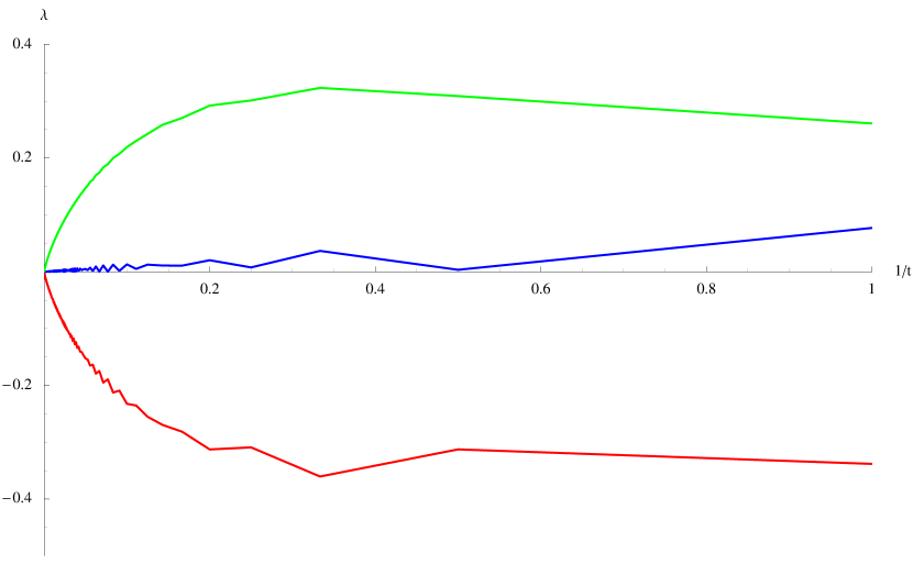
Figure 4.1: The Lyapunov exponents for the ABC flow in the integrable case $\mu=0$.

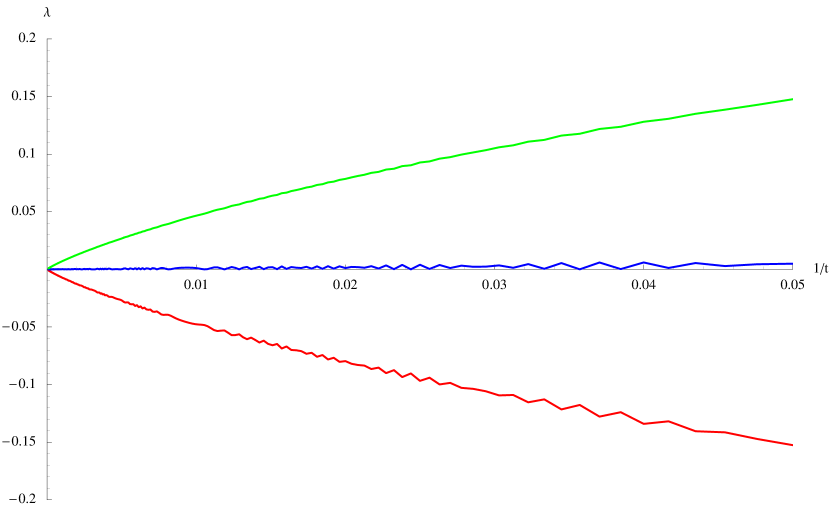
Figure 4.2: The Lyapunov exponents for the ABC flow in the integrable case ($\mu=0$) - a magnification of the $1/t=0$ vicinity.

The maximal value of $t$ was $10000$, and the values of the exponents at that point are

$$\lambda=(-9.173\times 10^{-4},9.099\times 10^{-4},7.404\times 10^{-7}).$$

Taking now the value of $\mu=1/2$ to investigate a non-integrable scenario, and the same initial conditions, the exponents can be seen to no longer all be zero, there is one tending to zero and two non zero of opposite signs, as it to be expected for a flow with conserved volume. Their values at $t=10000$ are

$$\lambda=(5.9\times 10^{-2},-5.886\times 10^{-2},-1.385\times 10^{-4}),$$

and their time dependence is shown in figures 4.3 and 4.4.

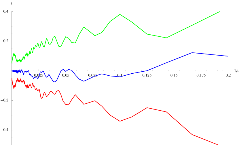
Figure 4.3: The Lyapunov exponents for the ABC flow in a non-integrable case $\mu=1/2$.

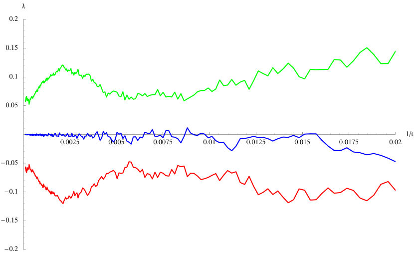
Figure 4.4: The Lyapunov exponents for the ABC flow in a non-integrable case ($\mu=1/2$) - a magnification of the $1/t=0$ vicinity.

When it comes to the variational equation, since there are no known first integral (a priori), we can only go as far as projecting it with respect to the trajectory. As shown in [11] there is a particular solution for which $y=\pi/4$, $z=x+\pi/2$, so that the trajectory is described by a single equation in $x(t)$ and gives as the projected VE

$$\dot{\xi} =\xi\sin(x)-2\mu\eta$$ (4.2)

$$\dot{\eta} =\xi\cos(x),$$

where $\xi$ and $\eta$ are the variations.

In the other approach, taking the coordinate basis $(\partial_{x},\partial_{y}\partial_{z})$ to be orthonormal, equation (3.79) becomes

$$\frac{\mathrm{d}}{\mathrm{d}s}{}_{\perp}\!Z^{\beta}=(\mathcal{A}^{\beta}_{\nu}-V^{\beta}\dot{V_{\nu}}){}_{\perp}\!Z^{\nu}.$$ (4.3)

which we want to change to involve time $t$, to compare it with the equations obtained above. Since the relation between the vectors is $\boldsymbol{W}=\left\langle\boldsymbol{W},\boldsymbol{W}\right\rangle\boldsymbol{V}$, the required derivations are rather cumbersome, but using the particular solution and the relation $\mathrm{d}s=\sqrt{\left\langle\boldsymbol{W},\boldsymbol{W}\right\rangle}\mathrm{d}t$, the above is finally reduced to

$${}_{\perp}\!\dot{Z}^{\beta}=\tilde{\mathcal{A}}^{\beta}_{\nu}{}_{\perp}\!Z^{\nu},$$ (4.4)

with

$$\tilde{\mathcal{A}}=\frac{A}{2}\begin{pmatrix}\sin(x)&-2\mu&-\sin(x)\\ 2\cos(x)&0&-2\cos(x)\\ -\sin(x)&2\mu&\sin(x)\end{pmatrix}.$$ (4.5)

This is in fact the same equation as before, when one defines $\xi$ to be ${}_{\perp}\!Z^{x}-{}_{\perp}\!Z^{z}$ and $\eta={}_{\perp}\!Z^{y}$ (in the cited paper the coefficient $A$ was taken to be 1). Obviously only two degrees of freedom are needed after the projection.

The geometric thus gives the same “starting” equation for further investigation. Its details – the determination of the differential Galois group can be found in the cited article.

4.2 $so(5)$ Gross-Neveu system

The Hamiltonian reads

$$H=\frac{1}{2}(p_{1}^{2}+p_{2}^{2})-2\cos(q_{1})-2\cos(q_{2})-4\cos(q_{1})\cos(q_{2}),$$ (4.6)

which translates into the appropriate vector $\boldsymbol{W}$

$$\frac{\mathrm{d}}{\mathrm{d}t}\begin{pmatrix}q_{1}\\ q_{2}\\ p_{1}\\ p_{2}\end{pmatrix}=\begin{pmatrix}p_{1}\\ p_{2}\\ -2\sin(q_{1})-4\sin(q_{1})\cos(q_{2})\\ -2\sin(q_{2})-4\cos(q_{1})\sin(q_{2})\end{pmatrix}.$$ (4.7)

As mentioned before, this system is never integrable meromorphically in the Liouville sense as shown it [12]. As the cited paper indicates, it has the interesting feature of appearing regular in the original variables, and clearly chaotic when a complex canonical transformation $q\rightarrow iq$, $p\rightarrow-ip$ is performed. The equations presented above are those after the transformation. In both cases the “effective” coordinates remain real, that is, when the initial conditions are real the variables remain real, and when they start as imaginary, they remain purely imaginary.

The first set of Lyapunov exponents was obtained for the imaginary domain (explicitly the above Hamiltonian) for the initial conditions of $q_{1}(0)=0.01$, $q_{2}(0)=0$, $p_{1}(0)=0.01$ and $p_{2}(0)$ positive, determined by the condition $H=3$. At the maximal time of $10000$ the spectrum was

$$\lambda=(0.2169,-0.2169,-2.64\times 10^{-3},2.64\times 10^{-3}).$$

It is clear that two of the exponents remain non zero as depicted in figure 4.5.

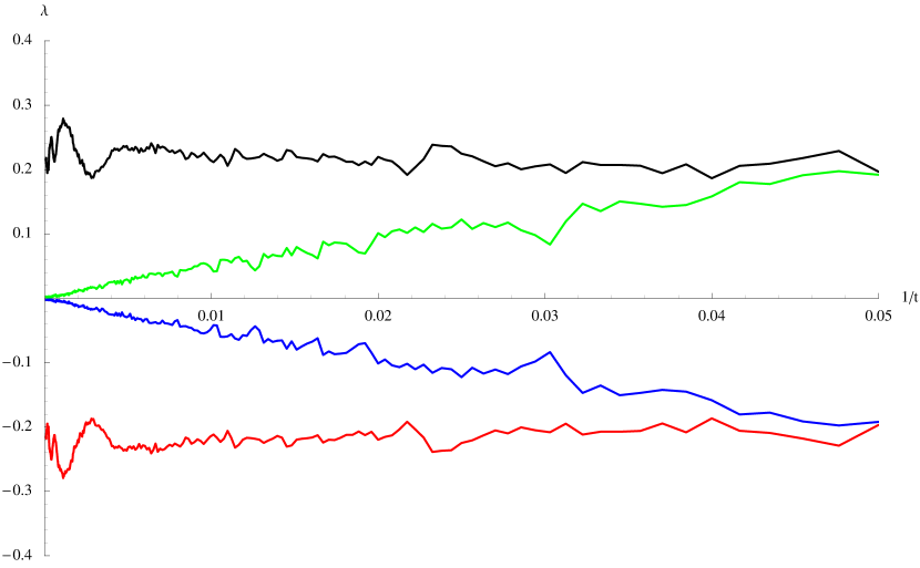
Figure 4.5: The Lyapunov exponents for the Gross-Neveu system in the imaginary domain.

For the real domain, where the Hamiltonian becomes

$$H=-\frac{1}{2}(p_{1}^{2}+p_{2}^{2})-2\cosh(q_{1})-2\cosh(q_{2})-4\cosh(q_{1})\cosh(q_{2}),$$ (4.8)

taking the initial conditions of $q_{1}(0)=0.01$, $q_{2}(0)=0$, $p_{1}(0)=0.01$ and $p_{2}(0)$ positive such that $H=-3$, the exponents all tend to zero with

$$\lambda=(1.753\times 10^{-3},-1.753\times 10^{-3},-3.651\times 10^{-4},3.651\times 10^{-4})$$

at $t=10000$. The results for this case is shown in figure 4.6.

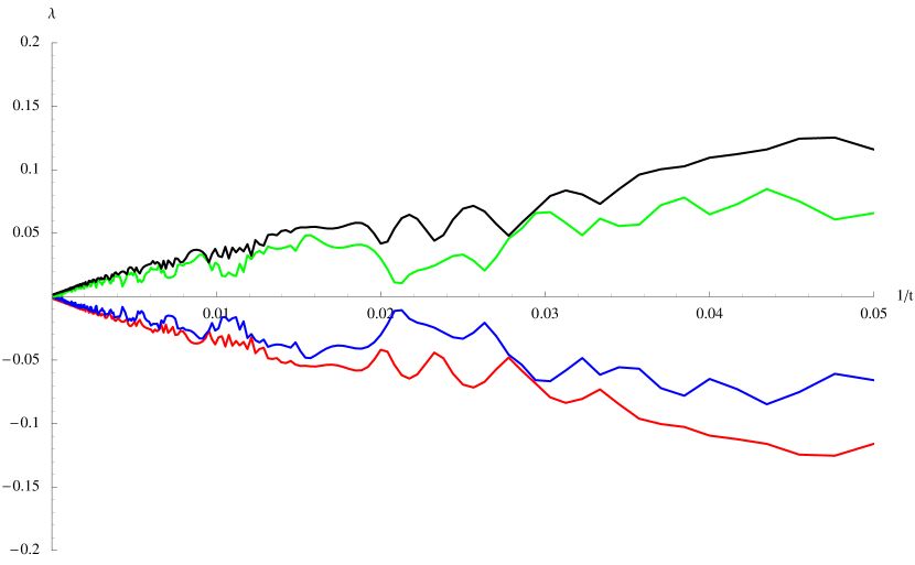
Figure 4.6: The Lyapunov exponents for the Gross-Neveu system in the real domain.

Let us see now how the double projection works to produce the normal variational equations in this case. In the algebraic approach the invariant plane $q_{2}=p_{2}=0$ is used to find a particular solution $(q_{1}(t),p_{1}(t))$, for which the Jacobian matrix of $\boldsymbol{W}$ is

$$A=\begin{pmatrix}0&0&1&0\\ 0&0&0&1\\ -6\cos(q_{1}(t))&0&0&0\\ 0&-2-4\cos(q_{1}(t))&0&0\end{pmatrix}.$$ (4.9)

Taking now only the variations in the directions $q_{2}$ and $p_{2}$ we get the NVE

$$\dot{\xi} =\eta$$ (4.10)

$$\dot{\eta} =-2-4\cos(q_{1}(t)),$$

where $\xi$ and $\eta$, as before, are the variations.

The geometric procedure is essentially the same as for the ABC flow, in that it consists of normalising the field $\boldsymbol{W}$, and the appropriate equation (3.80) is now

$${}_{\perp\!\!\!\perp}\!\dot{\boldsymbol{Z}}=\begin{pmatrix}-36f\sin^{2}(q_{1})&0&-6fp1\sin(q1)&0\\ 0&0&0&1\\ -6fp1\sin(q_{1})&0&-6fp_{1}^{2}&0\\ 0&-2-4\cos(q_{1})&0&0\end{pmatrix}{}_{\perp\!\!\!\perp}\!\boldsymbol{Z},$$ (4.11)

with

$$f=\frac{6p_{1}(6\cos(q_{1})-1)\sin(q_{1})}{(p_{1}^{2}+36\sin^{2}(q_{1}))^{2}}.$$ (4.12)

This is, again, the same as the algebraic NVE, when two of the degrees of freedom corresponding to $p_{1}$ and $q_{1}$ are suppressed. Alternatively one can check that the two vectors with respect to which the projection takes place, span the $p_{1}$, $q_{1}$ subspace, because on the trajectory

$$\boldsymbol{W} =(p1,0,-6\sin(q_{1}),0),$$ (4.13)

$$\boldsymbol{Y}=\sharp\mathrm{d}H =(6\sin(q_{1}),0,p1,0).$$

The above means that the next steps – checking if the NVE are soluble in the Liouvillian sense – is the same in both approaches. The proof that there are no such solutions can be found in the paper cited at the beginiing of this section.

4.3 Friedmann-Robertson-Walker cosmology

The last example is a cosmological system obtained for the FRW universe with a scalar field conformally coupled to gravity. It was analysed in great detail in [13], and includes both integrable and non-integrable sub-cases.

The particular Hamiltonian taken here is

$$H=\frac{1}{2}(p_{1}^{2}+p_{2}^{2})-\frac{1}{2}m^{2}q_{1}^{2}q_{2}^{2}+\frac{1}{4}(\Lambda q_{1}^{4}+\lambda q_{2}^{4}).$$ (4.14)

When

$$\Lambda=\lambda=-m^{2}$$

there is another first integral

$$J=q_{1}p_{2}-q_{2}p_{1},$$ (4.15)

and no additional integral exists if the parameters are varied slightly. It is thus convenient to substitute $m^{2}=-\lambda\epsilon$, so that the vector $\boldsymbol{V}$ is

$$\frac{\mathrm{d}}{\mathrm{d}t}\begin{pmatrix}q1\\ q2\\ p1\\ p2\end{pmatrix}=\begin{pmatrix}p1\\ p2\\ -\lambda q_{1}(q_{1}^{2}+q_{2}^{2}(1+\epsilon))\\ -\lambda q_{2}(q_{2}^{2}+q_{1}^{2}(1+\epsilon))\end{pmatrix}.$$ (4.16)

This example is used to show, that even though the system is integrable only when $\epsilon=0$, the Lyapunov exponents remain zero until the “perturbation” is big enough. Specifically, when $\epsilon=-1$, the spectrum at $t=10000$ is

$$\lambda=(-8.461\times 10^{-4},8.461\times 10^{-4},-7.909\times 10^{-4},7.909\times 10^{-4}).$$

Its time evolution is presented in figure 4.7. The initial conditions were $q_{1}(0)=0.01$, $q_{2}(0)=0$, $p_{1}(0)=0.01$ and $p_{2}(0)$ positive, determined by $H=0.01$.

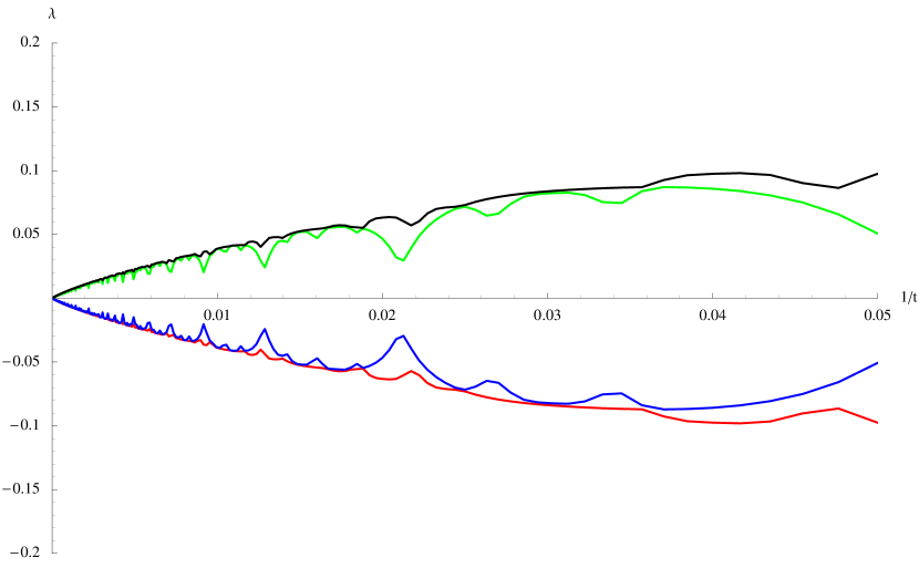
Figure 4.7: The Lyapunov exponents for the FRW system for $\epsilon=-1$.

Changing the value of $\epsilon$ to $-1.9$, with the same initial conditions gives a completely different picture. The exponents now read

$$\lambda=(-0.1388,0.1388,-8.078\times 10^{-4},8.078\times 10^{-4}).$$

This is to be expected for a Hamiltonian system – that the chaos becomes visible only for sufficient perturbation.

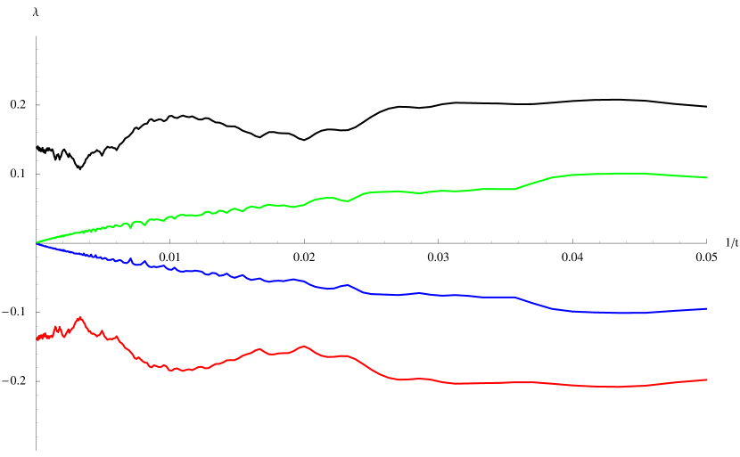
Figure 4.8: The Lyapunov exponents for the FRW system for $\epsilon=-1.9$.

Chapter 5 Final Matters

The study presented here can only be considered a beginning of further exploration of the subject, but it can be definitely said, that the two approaches – geometric and algebraic – can be successfully conflated to yield a better insight into integrability. Also, which is not to be underestimated, trying to use both descriptions immediately shows that some objects are ill-defined and some can be defined in many non-equivalent ways.

To be more concrete, the variations or small perturbations to a given dynamical system are an example of an object that reveals more when looked at from the geometric point of view. It is fundamentally different from the original system itself, as it really a vector on the tangent bundle of the main trajectory. It also turns out that it should commute with the vector field defining the system, as only then the transition to a nearby trajectory makes sense. It is also the only additional field we need to reconstruct the congruence of solutions if we can obtained the (first) variation as a function of the point on the manifold. As it is usually not the case, and we only solve an equation that gives the values of the variation on a particular trajectory, higher variations are needed.

Here also the basic notions of differential geometry are helpful to prove the existence of first integrals of the higher variational equations when the main system has a first integral. Unfortunately it appears, that higher variations, when defined to agree with the algebraic definitions, are not coordinate independent. A fact hard to notice when analysing the equation only in the coordinates in which it is introduced or obtained from physical considerations.

Another example of clear formulation is the Lyapunov matrix and the Lyapunov exponents. By definition they are constructed in a covariant way, but there is a price to pay for that. Namely the additional metric structure is required. Lyapunov exponents are usually computed using the time parameter that is naturally present in system of physical origin, but in general relativistic problems or those whose formulation admits the freedom of time reparametrisation it is not clear which variable is the real time. And it is obvious that a simple exponential change of that variable could make positive exponents zero [20].

The calculations presented here do not require any particular choice of metric, so that they can be applied to any case and guarantee consistency. On the other hand, without any particular choice it is impossible to obtain any results. That is why the examples included are treated as is usually the case – with the tacit assumption that the coordinates in which the system is defined are orthonormal. Until a distinguished metric structure can be canonically defined for dynamical systems (or at least the physical systems), this freedom of choice will remain unresolved.

As mentioned in the introduction there are attempts to geometrise the system by finding some metric which would make the equations be the geodesic equations on a suitable manifold, but so far this has been done for a small class of systems with natural kinetic energy. It also immediately collides with the problem of the base space – in the case of Jacobi metric for example, only the configuration space is taken into account, instead of the whole phase space.

This is best visible for Hamiltonian mechanics where we end up with analysing second order equations in the coordinates and the momenta (although also formally included in the solutions) do not play any role in the behaviour of neighbouring trajectories. Because the Jacobi geometrisation hinges heavily on the natural form of the kinetic energy, it is even impossible to obtain an analogous picture with a space of half the dimension involving only the momenta and suppressing the coordinates. The present work also shows that the symplectic structure of such systems requires some serious additional metric assumptions to speak about volume conservation. Even with the freedom that differential geometry gives, Hamiltonian systems become highly structured in this context.

Finally, among the still open problems, there is the question of studying more than just the Levi-Civita connection for which the results reduce to the algebraic ones. Introducing non-Riemannian (non-metric) connection or torsion, complicates the equations considerably, but has, seemingly, nothing to do with the question of integrability. This could hopefully give the possibility of investigating the system on many different manifolds and in fact obtaining different restrictions on integrability of the same basic equations.

Also, the algebraic tools are deeply rooted in the complex analysis of meromorphic functions, Riemann surfaces and analytic continuation. Thus, being integrable in the real sense is only understood indirectly. Here also lie new possibilities of extending the work to complex or Kähler manifolds, or developing the algebraic theory to treat the real-analytic case with more detail.

Bibliography

- [1] V. I. Arnold “Mathematical Methods of Classical Mechanics,” Springer-Verlag, New York, 1989.
- [2] M. Audin “Les Systèmes Hamiltoniens et leur Intégrabilité,” Cours Spécialisés, SMF et EDP-Sciences, 2001.
- [3] G. Benettin, L. Galgani, A. Giorgilli and J. M. Strelcyn “Lyapunov Characteristic Exponents for smooth dynamical systems and for hamiltonian systems; a method for computing all of them. Part 1: Theory,” Meccanica, 15, 1:9–20, 1980.
- [4] F. Beukers and A. van der Waall “Lamé equations with algebraic solutions.” J. Differential Equations, 197, 1–25, 2004.
- [5] M. Szydlowski “ The Eisenhart Geometry as an Alternative Description of Dynamics in Terms of Geodesics,” Gen. Rel. Grav., 30, 6:887–914, 1998.
- [6] A. Goriely “Integrability and Nonintegrability of Dynamical Systems,” World Scientific Publishing, Singapore, 2001.
- [7] G. Gorni and G. Zampieri “Analytic non-integrability of an integrable analytic Hamiltonian system,” Differ. Geom. Appl., 22, 3:287–296, 2005.
- [8] T. Kimura “On Riemann’s equations which are solvable by quadratures,” Funkcial. Ekvac., 12, 269–281, 1969.
- [9] S. Kobayashi and K. Nomizu “Foundations of Differential Geometry. Volume I,” Interscience Publishers, New York, 1963
- [10] J. J. Kovacic “An algorithm for solving second order linear homogeneous differential equations.” J. Symbolic Comput., 2, 1:3–34, 1986.
- [11] A. J. Maciejewski and M. Przybylska “Non-integrability of ABC flow,” Phys. Lett. A, 303, 4:265–272, 2002.
- [12] A. J. Maciejewski, M. Przybylska and T. Stachowiak “Non-integrability of Gross-Neveu systems,” Physica D, 201, 249–267, 2005.
- [13] A. J. Maciejewski, M. Przybylska, T. Stachowiak and M. Szydlowski “Global integrability of cosmological scalar fields,” arXiv:0803.2318, to appear in Journ. Phys. A
- [14] J. J. Morales-Ruiz “Differential Galois theory and non-integrability of Hamiltonian systems,” Birkhäuser Verlag, Basel, 1999.
- [15] J. J. Morales-Ruiz and J. P. Ramis “Integrability of Dynamical Systems through Differential Galois Theory: a practical guide,” preprint, 2007.
- [16] M. Przybylska “Differential Galois obstructions for integrability of homogeneous Newton equations,” Journ. Math. Phys., 49, 022701, 2008.
- [17] M. Przybylska “Finiteness of integrable -dimensional homogeneous polynomial potentials,” Phys. Lett. A, 369, 180–187, 2007.
- [18] M. Skwarczynski “Geometria rozmaitosci Riemanna,” PWN, Warszawa, 1993.
- [19] T. Stachowiak, A. J. Maciejewski and M. Szydlowski “Non-integrability of density perturbations in the FRW universe,” Journ. Math. Phys., 47, 032502, 2006.
- [20] M. Szydlowski “Toward an invariant measure of chaotic behaviour in general relativity,” Phys. Lett. A, 176, 1/2:22–32, 1993.
- [21] M. Szydlowski, M. Heller and W. Sasin “Geometry of spaces with the Jacobi metric,” J. Math. Phys., 37, 346, 1996.
- [22] A. Wolf, J. B. Swift, H. L. Swinney and J. A. Vastano “Determining Lyapunov exponents from a time series,” Physica D, 16, 285–315, 1985.
- [23] S. L. Ziglin “Branching of solutions and nonexistence of first integrals in Hamiltonian mechanics. I,” Funct. Anal. Appl., 16, 181–189, 1982.