Mid-Infrared Properties of Disk Averaged Observations of Earth with AIRS

Abstract

We have investigated mid-infrared spectra of Earth obtained by the Atmospheric Infrared Sounder (AIRS) instrument on-board the AQUA spacecraft to explore the characteristics that may someday be observed in extrasolar terrestrial planets. We have used the AIRS infrared (R $\sim$ 1200; 3.75-15.4 microns) spectra to construct directly-observed high-resolution spectra of the only known life bearing planet, Earth. The AIRS spectra are the first such spectra that span the seasons. We investigate the rotational and seasonal spectral variations that would arise due to varying cloud amount and viewing geometry and we explore what signatures may be observable in the mid-infrared by the next generation of telescopes capable of observing extrasolar terrestrial planets.

1 Introduction

Transit observations have recently been obtained for giant planets orbiting stars other than the sun (Deming et al., 2005; Charbonneau et al., 2002, 2005; Richardson et al., 2007; Swain et al., 2008; Tinetti et al., 2007) and there are plans for telescopes [e.g., TPFs (Terrestrial Planet Finders), JWST (James Webb Space Telescope), E-ELT (European Extremely large telescope)] that will be capable of observing terrestrial planets around other stars. Although the terrestrial planets around other stars likely have a broader range of characteristics than Earth or the other terrestrial planets in our solar system, so far, Earth is the only planet we know of that harbors life. Therefore it is necessary to explore the full range of spectral signatures and variability which can be observed for Earth, the only known life bearing planet, so that we can prepare for and understand the future observations of extrasolar terrestrial planets.

The Atmospheric Infrared Sounder (AIRS) on-board the AQUA spacecraft is an excellent tool with which to observe Earth. The AIRS obtains 2,916,000 spectra of Earth every day with 2378 Infrared channels in the wavelength range from 3.75 ${\rm\mu m}$ to 15.4 ${\rm\mu m}$ ($\lambda/\delta\lambda\sim 1200$) and 4 visible near-infrared channels (0.41–0.44 ${\rm\mu m}$; 0.58–0.68 ${\rm\mu m}$; 0.71–0.92 ${\rm mum}$; 0.49–0.94 ${\rm\mu m}$). The spacecraft has a polar Sun synchronous orbit with a 1:30 PM ascending equator crossing time. The spectra are obtained as the AIRS scans across its path from $\sim$ $-$49^∘ to $+$49^∘ about nadir from an altitude of $\sim$ 700 km. Thus, it is able to observe the entire Earth from space and provide a rich set of spectra consisting of day, night, land, ocean views at all latitudes. The radiometric calibration of AIRS has an uncertainty estimate of less than 0.2% in the mid-infrared and has been stable since launch (Olsen et al., 2007; Aumann et al., 2006).

Although future terrestrial planet finding telescopes must be designed so that they can characterize diverse types of terrestrial planets, Figure 1 shows that a relatively small region of Earth can display a large diversity of spectral features in the visible and infrared. However, since the first generation of terrestrial planet characterization missions will not spatially resolve the surface features on the planets they observe, only one spectrum will be observed for the whole visible disk. This paper examines the observable mid-infrared spectroscopic properties and Paper II (Hearty et al. 2008) examines the observable visible/near-infrared photometric properties.

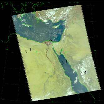
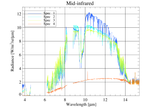
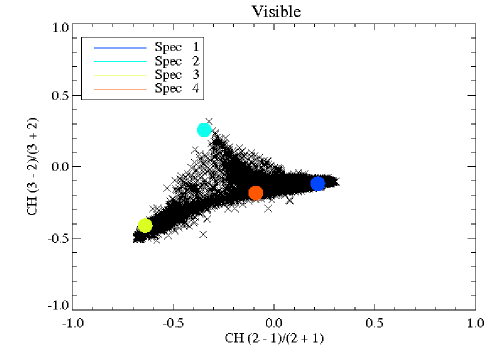
Figure 1: The top panel shows a visible image of a region observed with AIRS. The regions labeled 1-4 are the Sahara Desert, the Nile Delta, clear ocean, and cloud covered, respectively. The middle panel shows the mid infrared spectra from the regions labeled in the visible map. The bottom panel shows normalized visible/near-infrared channel differences (see Paper II) for all of the scenes in the figure with the 4 labeled regions indicated.

Whole Earth mid-infrared spectra have been directly obtained by the Galileo satellite (Sagan et al. 1993) and the Mars Global Surveyor satellite with the TES instrument (Christensen & Pearl, 1997). However, the spectral resolution of these investigations was not sufficient for detailed analysis and they only viewed Earth from a limited set of viewing geometries and seasons. “Earthshine” spectra are able to observe seasonal and rotational variations (Woolf et al., 2002; Pallé et al., 2003; Montañés-Rodriguez et al., 2005), however, they are limited to the visible near-IR region of the spectrum and they can only view earth edge-on. We have used directly observed spectra of Earth obtained with the AIRS to provide a detailed set of spectra to test existing models (Ford et al., 2001; Des Marais et al., 2002; Tinetti et al., 2005, 2006a, 2006b).

Although there is no reason to expect that we will observe a planet exactly like Earth or at the same evolutionary stage as Earth, the detailed spectra of Earth obtained by AIRS allow us to explore all of the biomarkers that may be seen when TPF-like missions observe an Earth-like planet orbiting another star. Thus, our AIRS spectra can serve as a library of sample spectra from a life-bearing habitable planet.

Section 2 describes the AIRS observations we used and how we converted the observed radiances to whole Earth spectra. We also compare a whole earth spectrum generated from AIRS to a TES/MGS observation of Earth for a similar season and viewing geometry from 1996. Section 3 describes the spectral signatures in the AIRS whole Earth spectra and what signatures will be observable with future telescopes capable of observing extrasolar terrestrial planets. Sections 4 and 5 examine the rotational and seasonal variations that could be detected in observations of an Earth-like extrasolar planet. Section 6 summarizes our findings.

2 Observations and Data Reduction

We investigated one day of AIRS spectra from the 26th of each month from September 26, 2004–August 26, 2005 using version 4 of the AIRS data products which are available from the Goddard Earth Sciences Data and Information Services Center. We placed the AIRS radiances onto the HEALPix grid (Górski et al., 2005) with Nside = 32 (12,288 pixels covering the earth). The HEALPix grid is an equal area grid that allows us to simulate how the Earth would look from different perspectives (e.g., edge-on and pole-on views) and easily calculate disk averaged spectra. Higher spatial resolution grids resulted in negligible differences in the disk averaged spectra. We produced grids to simulate (1) a “cloud-free” Earth and (2) a “fully cloud-covered” Earth using only clear or cloudy spectra culled from the full data set, and (3) a “normal” Earth using all of the data. We selected the clear and cloudy spectra by examining the AIRS “Level 2” data that provides an effective cloud fraction (CldFrcStd) for each scene. We defined “cloud-free” observations as those with a cloud fraction $<$ 0.05 and “fully cloud-covered” observations as those with a cloud fraction $>$ 0.95. Because of the paucity of observations that satisfy the clear (and cloudy) cases we used 4 days of AIRS observations to fill-in the grid before interpolating over the missing data.

Figure 2 shows global maps of the gridded data for the clear, normal, and cloudy cases. The clouds tend to mask surface features in the infrared brightness temperature maps of earth. Because Version 4.0.9.0 of the AIRS processing software sometimes misidentifies clear scenes as cloudy over very warm land, the significance of the masking of surface features is underestimated for some regions (e.g., the Sahara and Australia).

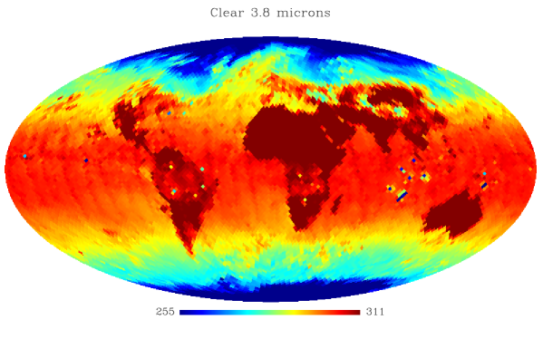
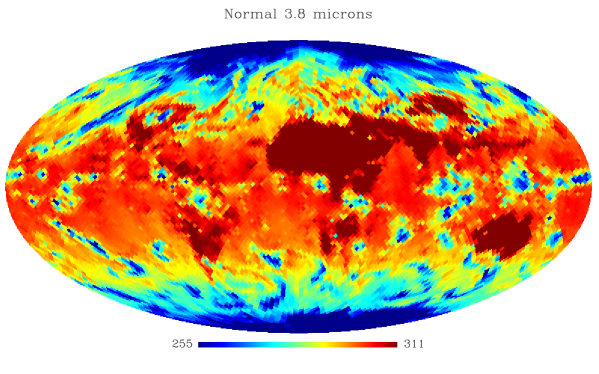
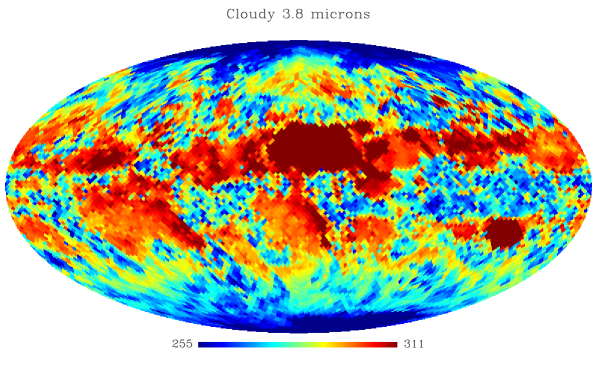
Figure 2: Maps of the daytime infrared brightness temperature [Kelvin] of the Earth at 3.8 $\mu$m (2616 cm^-1) are displayed for clear scenes (top), the actual earth (middle), and a cloud covered earth (bottom).

Since the AIRS data can be affected by cosmic rays, occasional noise events, and the South Atlantic Anomaly, we did not include any radiances with questionable calibration quality assessment parameters. Specifically, we only included radiances for which the CalFlag parameter is 0.

Figure 3 shows a comparison with a spectrum of Earth obtained with the TES instrument on the Mars global surveyor to AIRS whole earth spectra constructed for a similar viewing geometry for clear, normal, and cloudy cases from November 2004 and a normal cloud cover case from November 2005. The figure also includes a disc averaged spectrum calculated using a simple limb darkening parameterization adapted from Hodges et al. (2000) where the limb adjusted radiance R($\theta$) is calculated from the radiance at nadir R(0) as follows:

$$R(\theta)=\lambda(\theta)\times R(0),$$

where

$$\lambda(\theta)=1+0.09\times ln[cos(\theta)]$$

and $\theta$ is the zenith angle.

The observed differences between the AIRS and TES spectra could be due to slight differences in the assumed viewing geometry, cloud cover, limb effects, or calibration. Since there are differences between the AIRS spectra from November 2004 and November 2005 which have identical viewing geometries and calibration, we know that year-to-year spectral variations can be discerned. Although the simple limb darkening model seems to bring the AIRS and TES spectra into better agreement the observations made by the two instruments are separated by more than 10 years, thus the differences could also be due to changes in the cloud cover which can also significantly affect the spectra. A more accurate treatment of the limb effects is beyond the scope of this study. Moreover, since it is likely to be a small correction (relative to the effects of clouds), we neglect limb effects for the rest of this paper.

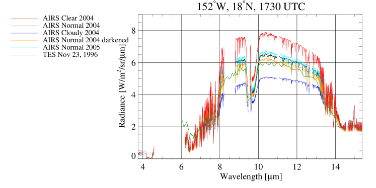
Figure 3: AIRS observations from November 26, 2004 and 2005 are compared with a TES observation of Earth from November 23, 1996.

3 Spectral Signatures

The mid-infrared observations with AIRS allow us to observe spectral signatures of habitability and life (e.g., H₂O, CO₂, CH₄, and an apparent temperature from the spectral shape). We used the 2004 HITRAN molecular transition line database to identify the spectral features from the AIRS data (Rothman et al. 2005). Figure 4 shows that for clear and cloudy scenes the O₃ line, an important sign of life can appear either in emission or absorption. Since the Earth contains regions that are clear and covered by dense clouds, the disk averaged AIRS spectra enable us to determine the limitations in characterizing the temperature of Earth-like planets with clouds. This effect can be significant since the variation in the mid-infrared due to clouds is greater than the differences between day and night. Figure 5 shows disk averaged broad-band mid-infrared spectra for fully illuminated and fully unilluminated views of earth on March 26, 2005 for clear, normal, and cloud covered cases. The “ocean view” is centered above the pacific with $\sim$ 10% of the projected area filled with land and the “land view” is centered above Africa with $\sim$ 40% of the projected area filled with land. The day night difference is larger over land than over ocean. We can also see from this figure that for an edge on view at opposition we will observe a larger radiance variation for a rotating planet with an uneven distribution of oceans and land (like Earth) than we will observe at conjunction.

Figure 6 shows the fully illuminated and unilluminated Earth spectra of the H₂O, O₃, CO₂, and CH₄ spectral features and the ratio of the spectral feature in the daytime and the night time. The 14 $\mu$m CO₂ feature is less sensitive to day night difference and varying cloud amounts than the 4 $\mu$m CO₂ lines that include some reflected sunlight. However, the saturated line cores of O₃ and CO₂ due to the warm stratosphere are similar for both the clear and cloudy cases. Therefore, if an earth-like extrasolar planet were completely covered by clouds we may still be able to detect O₃ emission if the telescope has sufficient spectral resolution.

Since the first generation of telescopes capable of directly detecting spectra of extrasolar terrestrial planets will likely not have the spectral resolution of AIRS many of the features seen in the spectra described in this paper may not be observable. The space-based NASA-Terrestrial Planet Finder mission concepts (TPF-O, TPF-C, TPF-I) or the ground-based European Extremely Large Telescope (E-ELT) are expected to image and characterize exoplanets down to Super-Earth and Earth-size. In these cases, the spectral resolution obtainable will be limited by the photon noise, so a reasonable estimate is a spectral resolution of $\sim$ 50 for super-Earths at 10 pc. Higher spectral resolution spectra in the Infrared, though, could be obtained with JWST for super-Earths in the habitable zone of M stars using the secondary transit technique.

Figure 7 displays AIRS disk averaged spectra degraded to spectral resolutions of R = 100, 50, and 25. Molecular absorption lines of H₂O, O₃, CO₂, and CH₄ are detectable in all but the most cloudy cases. However, the emission lines due to stratospheric O₃ and CO₂ are only detectable in the spectra with R $=$ 100.

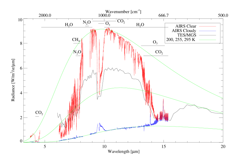
Figure 4: Radiance spectra of two $\sim$ 15 km views of Earth obtained with AIRS are displayed with a disk averaged spectrum of Earth obtained with TES/MGS and three black body curves. Black body fitting can give the surface temperature but the spectral lines may be in absorption, emission, or not present.

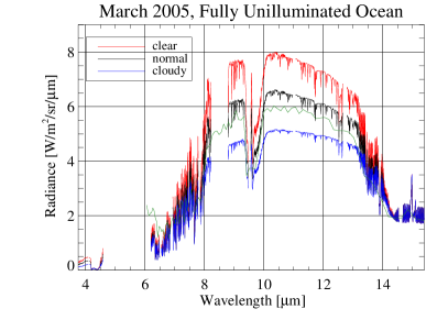
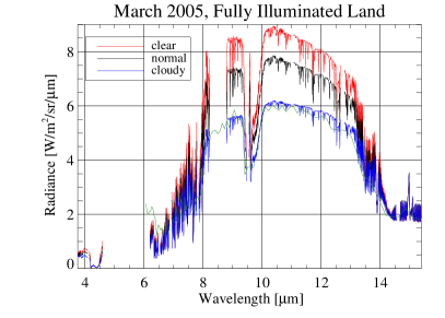
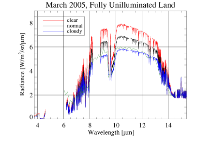
Figure 5: Clear, Normal, and cloudy whole earth spectra are displayed for 4 views of Earth on March 25, 2005: Fully Illuminated Ocean (top left), Fully Unilluminated Ocean (top right), Fully Illuminated Land (bottom left), and Fully Unilluminated Land (bottom right). The spectral variation due to clouds is larger than the differences between day, night, land, or ocean. The projected land fraction for the “ocean” case is $\sim$ 10% and the projected land fraction for the “land” case is $\sim$ 40%

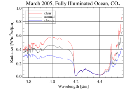
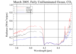
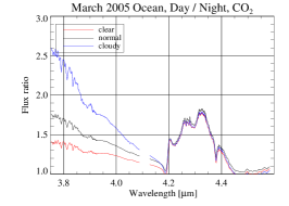
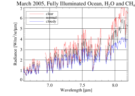
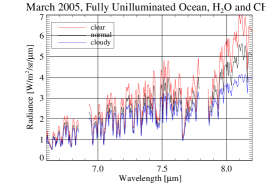
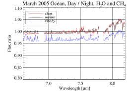
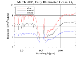
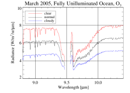
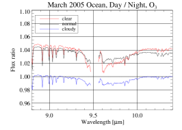
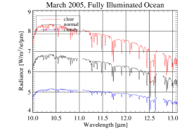
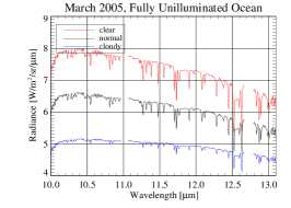
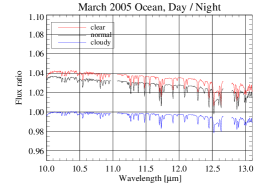
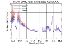
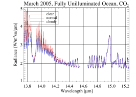
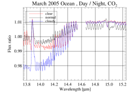
Figure 6: Five spectral regions (from top to bottom) are shown for disk averaged spectra of an edge on view of Earth that is (1) fully illuminated “day” and (2) unilluminated “night” ocean views and (3) the ratio between day and night (from left to right). The weak lines between 3.8 and 4.0 $\mu m$ are due to HDO and the large ratio between day and night in this region is due to reflected solar radiation which is more significant for the cloudy cases. Absorption lines of CO₂, O₃, H₂O, and CH₄ are clearly seen. The CO₂ and O₃ emission lines are due to stratospheric emission. The lines from 10-13 $\mu m$ are due to H₂O and the slope in this region may be an indicator of water even if the lines are not resolved.

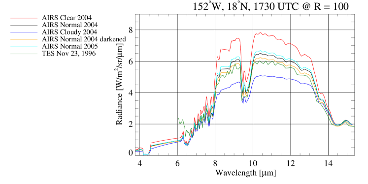
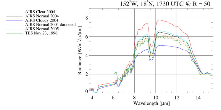
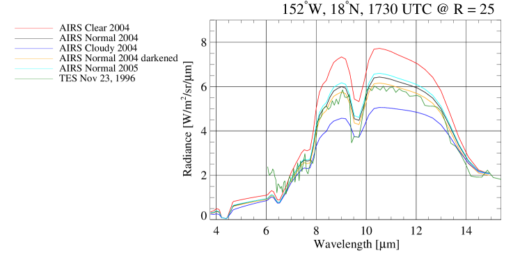
Figure 7: The 3 panels show the same as Figure 3 with the spectral resolution degraded to R = 100, 50, and 25 (from top to bottom).

4 Rotational Variations

Figure 5 has already shown that fully illuminated “daytime” spectra show larger rotational variations depending upon the amount of land in the field of view and the daytime absorption features are deeper than in the unilluminated “nighttime” spectra. However, telescopes like TPF and Darwin will not observe planets that are fully illuminated or fully unilluminated since the planets must be away from their star. A more likely observing scenario would be for the planet to be partially illuminated. Thus, we examine the rotational radiance variations due to planet rotation by creating disk averaged spectra for edge-on and pole-on viewing geometries in two hour increments (UT = 0–23 hours).

Figure 8 shows an edge-on view of Earth seen in March from a distant observer located at RA = 6.0 hours & Dec = 23.5^∘, the “Summer Solstice” view. The spectral features (e.g., O₃, H₂O, CO₂, and CH₄) are visible at all times and the amplitude of the variability in the continuum is $\sim$ 10% as calculated by Des Marais et al. (2002). The magnitude of the radiometric variability is probably exaggerated for the cloudy cases since some clear scenes over the Sahara were misidentified as cloudy.

Figure 9 shows a nearly pole-on view of Earth as seen by an observer located at RA = 14.6 hours & Dec = $-$60.63^∘, the “$\alpha$ Centauri” view. The same spectral lines are visible but the spectra are colder and the amplitude of the radiometric variability is reduced. A similar pole-on view of the northern hemisphere shows a larger rotational variability because of the larger fraction of land in the northern hemisphere.

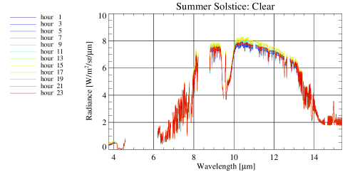
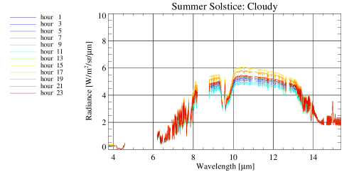
Figure 8: Infrared spectra are displayed for clear, normal, and cloudy scenes for an edge-on viewing geometry on March 26, 2005.

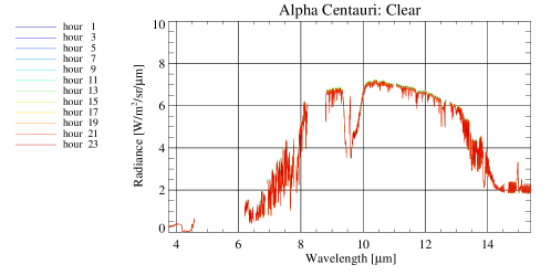
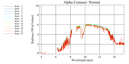
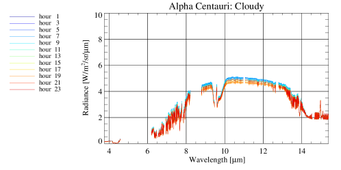
Figure 9: Infrared spectra are displayed for clear, normal, and cloudy scenes for a nearly pole-on viewing geometry of Earth viewed from $\alpha$ Centauri on March 26, 2005.

5 Seasonal Variations

Although the whole seasonal cycle will not be observable by TPF or Darwin for edge-on views because the planet will be too close to the star for some cases (e.g., eclipsing planets) spectra may be obtained by other means. Specifically the transit method makes it possible to study the atmosphere of the transiting planet. In particular, the secondary eclipse (when the planet is blocked by its star) allows a direct measurement of the planet’s radiation. If the star’s contribution during the secondary eclipse is subtracted from the observed spectrum before or after, only the signal caused by the planet remains. It is then possible to measure the planet’s emitted (Deming et al., 2005; Charbonneau et al., 2002) or reflected spectrum (Rowe et al., 2006) depending on the wavelength region selected for the observations. Pole-on views will be observable for all seasons provided there is sufficient separation between the star and planet. If the planet is tilted with respect to its orbit and there is an uneven distribution of land and sea (like Earth) we expect to see seasonal variations in the temperature and perhaps atmospheric gases. For a life bearing planet, seasonal variations in O₃ & CO₂ may even be indicators of life. We simulated 24 hour integrations by averaging the radiances observed over a 24 hour period and did this for 12 months from September 2004 – August 2005.

Figure  10 shows the seasonal variations in the mid-infrared for a view of Earth from RA = 6.0 hours & Dec = 23.5^∘, the “Summer Solstice” view. The major spectral features in the mid infrared are visible for all seasons even for the cloud covered cases. Since this edge-on view is shifted slightly to the northern hemisphere, there is also a significant seasonal radiometric variability due to the heating of the land in the boreal summer.

Figure  11 shows the seasonal variations in the mid-infrared for a view of Earth from RA = 14.6 hours & Dec = $-$60.63^∘, the “$\alpha$ Centauri” view. The major spectral features in the mid infrared are visible for all seasons but the H₂O lines are weaker for the more cloudy cases. Since this nearly pole-on view is shifted to the southern hemisphere the warmest spectrum is in the austral Summer. However, since there is less land in the southern hemisphere, the amplitude of the seasonal radiometric variability is less than for views that see the northern hemisphere.

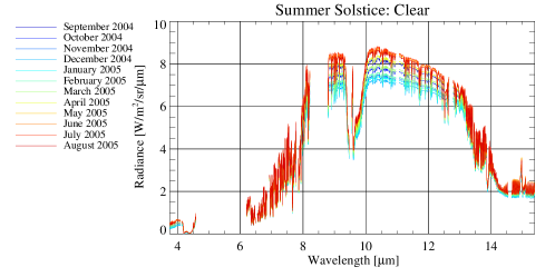
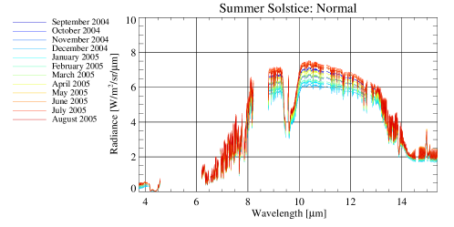
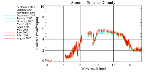
Figure 10: The Seasonal variations are displayed for edge-on views of Earth for Clear, Normal, and Cloudy cases.

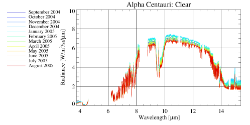
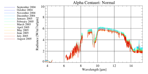
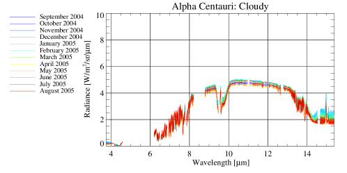
Figure 11: The Seasonal variations are displayed for 3 pole-on views of Earth for Clear, Normal, and Cloudy cases.

6 Conclusions

Cloud amount and patchiness will be the most observable characteristic of extrasolar Earth-like planets in the mid-infrared since clouds can alter the apparent temperature and the detectability of mid-infrared spectral features that are tracers for habitability and life. Viewing geometry can have a similar effect. Molecular lines of H₂O, CH₄, CO₂, and O₃ are detectable in the disk averaged spectra of all geometries and cloud amounts examined. However, he robustness of the detections degrades at lower spectral resolution particularly for cloudier cases.

If an extrasolar planet is completely covered with cloud, O₃ and CO₂ may not appear in absorption even if they are present. However, the lines may appear in emission if they are present above the cloud layer and observed with sufficient spectral resolution (R $\sim$ 100).

The AIRS observations confirm that rotational and seasonal variations in the mid-infrared can be as large as $\sim$ 10% for a planet with a tilted rotation axis and an uneven distribution of land and ocean. However, the amplitude of this variability may be reduced for some viewing geometries and cloud coverage. The rotational variations in the infrared and visible may be used to infer the period of the planet.

References

- Aumann et al. (2006) Aumann, H. H., Broberg, S., Elliott, D., Gaiser, S., & Gregorich, D. 2006, Journal of Geophysical Research (Atmospheres), 111, 16
- Charbonneau et al. (2002) Charbonneau, D., Brown, T. M., Noyes, R. W., & Gilliland, R. L. 2002, ApJ, 568, 377
- Charbonneau et al. (2005) Charbonneau, D., et al. 2005, ApJ, 626, 523
- Christensen & Pearl (1997) Christensen, P. R., & Pearl, J. C. 1997, J. Geophys. Res., 102, 10875
- Deming et al. (2005) Deming, D., Seager, S., Richardson, L. J., & Harrington, J. 2005, Nature, 434, 740
- Des Marais et al. (2002) Des Marais, D., Harwit, M., Jucks, K, Kasting, J., Lunine, J., Lin, D., Seager, S., Schneider, J., Traub, W., Woolf, N., 2002, “Biosignatures and Planetary Properties to be Investigated by the TPF Mission,” JPL Publication 01-008, Rev. A.
- Ford et al. (2001) Ford, E. B., S. Seager, and E. L. Turner. 2001. Characterization of extrasolar terrestrial planets from diurnal photometric variability, Nature, 412, 2001, 885-887.
- Górski et al. (2005) Górski, K. M., Hivon, E., Banday, A. J., Wandelt, B. D., Hansen, F. K., Reinecke, M., & Bartelmann, M. 2005, ApJ, 622, 759.
- Hodges et al. (2000) Hodges, K.I., Chappell, D.W., Robinson, G.J., and Yang, G. An Improved Algorithm for Generating Global Window Brightness Temperatures from Multiple Satellite Infrared Imagery, Journal of Atmospheric and Oceanic Technology, 17, 2000, 1296-1312.
- Montañés-Rodriguez et al. (2005) Montañés-Rodriguez, P., Pallé, E., Goode, P., Hickey, J., Koonin, S, Globally Integrated Measurements of the Earth’s Visible Spectral Albedo, ApJ, 629, pp. 1175-1182
- Olsen et al. (2007) Olsen, E.T., Fetzer, E., Lee, S-Y., Manning, E., Blaisdell, J., Susskind, J., AIRS/AMSU/HSB Version 5 CalVal Status Summary, 2007, Available online at: http://disc.gsfc.nasa.gov/AIRS/documentation/v5_docs/AIRS_V5_Release_User_Docs/V5_CalVal_Status_Summary.pdf.
- Pallé et al. (2003) Pallé, E., et al. 2003, Journal of Geophysical Research (Atmospheres), 108, A13
- Richardson et al. (2007) Richardson, L.J., Deming, D., Horning, K., Seager, S., Harrington, J., Nature, 445, 892.
-
Rothman et al. (2000)
L.S. Rothman; , A. Barbe, D. Chris Benner, L.R. Brown, C. Camy-Peyret, M.R. Carleer , K. Chance, C. Clerbaux, V. Dana,
V.M. Devi, A. Fayt, J.-M. Flaud, R.R. Gamache, A. Goldman, D. Jacquemart, K.W. Jucks, W.J. Lafferty, J.-Y. Mandin,
S.T. Massie, V. Nemtchinov, D.A. Newnham, A. Perrin, C.P. Rinsland, J. Schroeder, K.M. Smith, M.A.H. Smith, K. Tang,
R.A. Toth, J. Vander Auwera , P. Varanasi, K. Yoshino,
The HITRAN molecular spectroscopic database: edition of 2000 including updates through 2001,
Journal of Quantitative Spectroscopy & Radiative Transfer §2 (2003) 5-44 - Rowe et al. (2006) Rowe, J. F., et al. 2006, Memorie della Societa Astronomica Italiana, 77, 282.
- Sagan et al. (1993) Sagan, C., Thompson, W.R., Carlson, R., Gurnett, D., Hord, C., 1993, Nature 365, 715.
- Swain et al. (2008) Swain, M., Bouwman, J., Akeson, R.L., Lawler, S., Beichman, C.A., 2008, The Mid-infrared Spectrum of the Transiting Exoplanet HD 209458b, ApJ, 674, 482.
- Tinetti et al. (2005) Tinetti, G., Meadows, V.S., Crisp, D., Fong, W., Velusamy, T., & Snively, H; Disk-averaged synthetic spectra of Mars, Astrobiology, Volume 5, Number, 2005
- Tinetti et al. (2006a) Tinetti, G., Meadows, V. S., Crisp, D., Fong, W., Fishbein, E., Turnbull, M., & Bibring, J.-P. 2006, Astrobiology, 6, 34
- Tinetti et al. (2006b) Tinetti, G., Meadows, V. S., Crisp, D., Kiang, N. Y., Kahn, B. H., Fishbein, E., Velusamy, T., & Turnbull, M. 2006, Astrobiology, 6, 881
- Tinetti et al. (2007) Tinetti, et al. 2007, Nature, 448, 169.
- Woolf et al. (2002) Woolf, N.J., Smith, P.S., Traub, W.A., & Jucks, K.W. 2002, ApJ, 574, 430