Quasispecies Theory for Horizontal Gene Transfer and Recombination

Abstract

We introduce a generalization of the parallel, or Crow-Kimura, and Eigen models of molecular evolution to represent the exchange of genetic information between individuals in a population. We study the effect of different schemes of genetic recombination on the steady-state mean fitness and distribution of individuals in the population, through an analytic field theoretic mapping. We investigate both horizontal gene transfer from a population and recombination between pairs of individuals. Somewhat surprisingly, these nonlinear generalizations of quasi-species theory to modern biology are analytically solvable. For two-parent recombination, we find two selected phases, one of which is spectrally rigid. We present exact analytical formulas for the equilibrium mean fitness of the population, in terms of a maximum principle, which are generally applicable to any permutation invariant replication rate function. For smooth fitness landscapes, we show that when positive epistatic interactions are present, recombination or horizontal gene transfer introduces a mild load against selection. Conversely, if the fitness landscape exhibits negative epistasis, horizontal gene transfer or recombination introduce an advantage by enhancing selection towards the fittest genotypes. These results prove that the mutational deterministic hypothesis holds for quasi-species models. For the discontinuous single sharp peak fitness landscape, we show that horizontal gene transfer has no effect on the fitness, while recombination decreases the fitness, for both the parallel and the Eigen models. We present numerical and analytical results as well as phase diagrams for the different cases.

I Introduction

It has been argued that genetic recombination provides a mechanism to speed up evolution, at least in finite populations Cohen et al. (2005). Moreover, it has been suggested that recombination may provide a way to escape from the phenomenon of “Muller’s ratchet” Muller (1964), or suboptimal fitness characteristic of finite populations with asexual reproduction. In bacteria, it has been proposed Lawrence (1997) that horizontal gene transfer allows for the gradual emergence of modularity, through the formation of gene clusters and their eventual organization into operons. In in-vitro systems, protein engineering protocols by directed evolution incorporate genetic recombination in the form of DNA shuffling Patten et al. (1997); Lutz and Benkovic (2000) to speed up the search for desired features such as high binding constants among combinatorial libraries of mutants.

Besides these inherently dynamical effects, it remains a matter of debate if the exchange of genetic-encoding elements provides a long-term advantage to an infinite population in a nearly static environment. Indeed, it is argued that Otto and Lenormand (2002) when advantageous genetic associations have been generated as a result of selection in a given environment, further random recombination is likely to disrupt these associations, thus decreasing the overall fitness. This argument is less cogent if we consider that recombination and horizontal gene transfer preserve the modular structure of the genetic material Lawrence (1997). That is, entire operational and functional units are recombined, rather than random pieces. It has also been proposed that for recombination to introduce an advantage in infinite populations, negative linkage disequilibrium is required Arjan et al. (2007); Misevic et al. (2006); Kondrashov (1982, 1993). This situation means that particular allele combinations are present in the population at a lower frequency than predicted by chance. Negative linkage disequilibrium can result as a consequence of negative epistasis: alleles with negative contributions to the fitness interact synergistically, increasing their deleterious effect when combined, and alleles with positive contributions to the fitness interact antagonistically Azevedo et al. (2006); Arjan et al. (2007); Phillips et al. (2000), see Fig. 1. Under negative epistasis, the mutational deterministic hypothesis Kimura and Maruyama (1966); Kondrashov (1982, 1988, 1993); Arjan et al. (2007); Azevedo et al. (2006); Kouyos et al. (2007) postulates that recombination promotes a more efficient removal of deleterious mutations, by bringing them together into single genomes, and hence facilitating selection Kimura and Maruyama (1966); Rice and Chippindale (2001) to discard those genotypes with low fitness. It has been argued that the negative linkage disequilibrium generated by negative epistatic interactions is a factor to promote the evolution of recombination in nature Arjan et al. (2007); Kouyos et al. (2007, 2006), and conversely that recombination may act as a mechanism to evolve epistasis Liberman and Feldman (2005); Liberman et al. (2007); Liberman and Feldman (2008). This later statement is controversial, since it is intuitive that recombination should contribute to weaken correlations between different genes Malmberg (1977). Despite these theoretical arguments, experimental studies seem to indicate that negative epistasis is not so common in nature Bonhoeffer et al. (2004); Wloch et al. (2001) as recombination and, moreover, both negative and positive epistasis may coexist as different fitness components Arjan et al. (2007) within the same genome in natural organisms.

To address some of these questions, we study the effect of transferring genetic information between different organisms in an infinite population. We choose the conceptual framework of “quasi-species” theory, represented by two classical models of molecular evolution: the Eigen Eigen and Schuster (1971); Eigen et al. (1988, 1989); Biebricher and Eigen (2005) model and the parallel, or Crow-Kimura, model Crow and Kimura (1970); Baake and Wagner (2001). These classical models include the basic processes of mutation, selection, and replication that occur in biological evolution. Our goal is to solve these two standard models of quasi-species theory, Crow-Kimura and Eigen, when horizontal gene transfer or recombination are included. Since horizontal gene transfer and recombination are essential features of evolutionary biology, our solutions bring quasi-species theory closer to modern biology. An operational definition of fitness is provided in these models by the replication rate, which is considered to be a function of the genotype. In their simplest formulation quasi-species models consider a static environment, with a deterministic mapping between individual genetic sequences and replication rate. Both the Eigen Eigen and Schuster (1971); Eigen et al. (1988) and the parallel, or Crow-Kimura model Crow and Kimura (1970), are formulated in terms of a large system of differential equations, describing the time evolution of the relative frequencies of the different sequence types in an infinite population, a mathematical language that is common in the field of chemical kinetics Eigen and Schuster (1971); Eigen et al. (1988). Sequences, representing information carrying molecules such as RNA or DNA, are assumed to be drawn from a binary alphabet (e.g. purines/pyrimidines). The most remarkable property of these classical models is that when the mutation rate is below a critical value they exhibit a phase transition in the infinite genome limit Eigen and Schuster (1971); Eigen et al. (1988, 1989); Tarazona (1992); Leuthausser (1987); Biebricher and Eigen (2005); Franz and Peliti (1997); Park and Deem (2006); Saakian et al. (2006), with the emergence of a self-organized phase: the quasi-species Eigen and Schuster (1971); Eigen et al. (1988, 1989). This organized phase, characterized by a collection of nearly neutral mutants rather than by a single homogeneous sequence type, is mainly a consequence of the auto-catalytic character of the evolution dynamics, which tends to enrich exponentially the proportion of fittest individuals in the population Eigen and Schuster (1971); Eigen et al. (1988, 1989); Biebricher and Eigen (2005). The quasi-species concept, with its corresponding ”error threshold” transition, has been applied in the interpretation of experimental studies in RNA viruses Domingo et al. (1978, 2005); Ortin et al. (1980); Domingo et al. (1985). In particular, the error-threshold transition has been proposed as a theoretical motivation for an antiviral strategy Eigen (2002), termed ”lethal mutagenesis”, which drives an infecting population of viruses towards extinction by enhancing their mutation rate Graci et al. (2007); Loeb et al. (1999); Loeb and Mullins (2000). It has been argued, however, that the mechanism for lethal mutagenesis possesses a strong ecological component Bull et al. (2007), and that perhaps the mean population fitness is simply driven negative, and so the total number of viral particles in an infecting population decreases in time towards extinction, in contrast with error-threshold theories that describe a randomization of the composition of the quasi-species in genotype space.

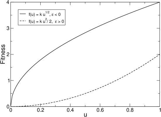
Figure 1: Convention for the sign of epistasis, $\epsilon$. In the figure are represented two smooth fitness landscapes, as a function of $u=2l/N-1$, with $N$ the total length of the (binary) genetic sequences and $0\leq l\leq N$ the number of beneficial mutations (number of ’+’ spins) along the sequence. In this representation, positive (synergistic) epistasis $\epsilon>0$ corresponds to a positive curvature $f^{{}^{\prime\prime}}(u)>0$, while negative (antagonistic) epistasis $\epsilon<0$ corresponds to a negative curvarture $f^{{}^{\prime\prime}}(u)<0$ Phillips et al. (2000); Azevedo et al. (2006); Arjan et al. (2007). The examples shown are a quadratic fitness landscape $f(u)=ku^{2}/2$ (dashed line), with positive curvature and $\epsilon>0$, and a square-root fitness landscape $f(u)=k\sqrt{u}$ (solid line), with negative curvature and $\epsilon<0$. We set $k=4.0$ in both examples.

The existence of the error threshold transition has motivated the attention of theoretical physicists, especially since it was proved that the quasi-species theory can be exactly mapped into an 2D Ising spin system Leuthausser (1987); Tarazona (1992), with a phase transition that is first order for a sharp peak fitness, and second or higher order for smooth fitness functions. More recently, exact mappings into a quantum spin chain Baake et al. (1997, 1998); Saakian and Hu (2006); Saakian et al. (2004); Saakian and Hu (2004) or field theoretic representations Park and Deem (2006) have been developed. Analytical and numerical studies of these systems, in the large genome limit, are possible when the fitness function is considered to be permutation invariant Baake et al. (1997, 1998); Park and Deem (2006, 2007); Franz and Peliti (1997), or depending on the overlap with several peaks in sequence space Saakian et al. (2006). The mapping of the quasi-species models into a physical system allows for the application of the powerful mathematical techniques of statistical mechanics, thus obtaining exact analytical solutions which provide significant insight over numerical studies Park and Deem (2006); Saakian et al. (2006); Saakian and Hu (2006). Most of the existing analytical solutions correspond to the case when recombination is absent. Recombination and horizontal gene transfer have been studied by computer simulations of artificial gene networks Azevedo et al. (2006) and digital organisms Misevic et al. (2006), but relatively few analytical approaches have been reported in the context of quasi-species theory Boerlijst et al. (1996); Cohen et al. (2005); Park and Deem (2007); Jacobi and Nordahl (2006). A numerical study of a mathematical model for viral super-infection termed uniform crossover, and intermediate between horizontal gene transfer and recombination, has been reported Boerlijst et al. (1996), with numerical solutions based on relatively short viral sequences (N=15). More recently, the effect of incorporating horizontal gene transfer in quasi-species theory has been studied in terms of the dynamics Cohen et al. (2005), reporting numerical studies and approximate analytical expressions. Exact analytical expressions for the equilibrium properties of the population in the presence of horizontal gene transfer have been derived using the methods of quantum field theory Park and Deem (2007).

In this article, we study the effect of introducing different schemes of genetic recombination in quasi-species theory. Extending the results in Park and Deem (2007), we present an exact field theoretical mapping of the parallel and Eigen models. We remark that field theoretical methods provide a unique and powerful set of tools for the analytical study of dynamical systems, such as reaction-diffusion Lee and Cardy (1995); Mattis and Glasser (1998) or birth-death processes Peliti (1985). In this paper, we employ these theoretical tools to obtain exact analytical expressions for the equilibrium mean fitness and average composition of the population, for permutation invariant but otherwise arbitrary replication rate functions.

In Section 2 we consider the parallel model. We consider horizontal gene transfer of non-overlapping blocks, as well as of blocks of random size. We also consider a recombination process producing a daughter sequence symmetrically from two parents, as might occur in viral super- or co-infection. In Section 3, we study the effect of these different genetic recombination schemes in the context of the Eigen model. In both models, recombination leads to two selected phases. Interestingly, beyond a critical recombination rate, the distribution of the population becomes independent of the recombination rate. Also interesting is that the steady-state distribution is independent of the crossover probability.

To study the effect of epistasis, whose sign is determined by the curvature of the fitness landscape (second derivative) when represented as a function of the Hamming distance with respect to the wild-type, we considered two different examples of smooth fitness functions: a quadratic function, representing positive epistasis, and a square-root function representing negative epistasis. We find that, for the quadratic fitness function, horizontal gene transfer and recombination introduce a mild load against selection. The opposite effect is observed for the square-root fitness, that is, horizontal gene transfer and recombination introduce an advantage by enhancing selection towards fittest genotypes. This results provide support for the mutational deterministic hypothesis, which postulates that recombination should be beneficial for negative epistasis fitness functions, and deleterious for positive epistasis fitness functions. Moreover, we prove analytically in Appendix L that the mutational deterministic hypothesis applies for the parallel model in the presence of horizontal gene transfer. A similar proof is provided in Appendix M for the Eigen model. We also show analytically that the mutational deterministic hypothesis applies for the case of two-parent recombination, as presented in Appendix N for the parallel model, and in Appendix O for the Eigen model.

The effect of recombination becomes negligible for discontinuous fitness landscapes, such as a single sharp peak. For all these cases, we present exact analytical expressions that determine the phase structure of the population at steady state. Results are explicit for any microscopic fitness function: Eqs. (14), (31), and (62–63) for the parallel model and Eqs. (82), (93), and (106–107) for the Eigen model. We evaluate these expressions for three permutation invariant fitness functions: sharp peak, quadratic, and square root for the two common forms of quasi-species theory, parallel and Eigen: Eqs. (22), (23), (33), (34), (68), (71), (85–87), (96–98), (112), and (113). We also present numerical tests supporting our analytical equations.

II The parallel model

We consider a generalization Park and Deem (2007) of the parallel, or Crow-Kimura Crow and Kimura (1970), model to take into account the transfer of genetic material between pairs of individuals in an infinite population.

$$\frac{dq_{i}}{dt}=r_{i}q_{i}+\sum_{k=1}^{2^{N}}\mu_{ik}q_{k}+\nu N\frac{\sum_{k,l}R^{i}_{kl}q_{k}q_{l}}{\sum_{k}q_{k}}-\nu Nq_{i}$$ (1)

Here, $q_{i}$ represents the (unnormalized) frequency of the sequence type $S_{i}=(s_{1}^{i},s_{2}^{i},\ldots,s_{N}^{i})$, with $s_{j}^{i}=\pm 1$, for $1\leq i\leq 2^{N}$ and $1\leq j\leq N$. The normalized frequencies are obtained from $p_{i}=q_{i}/\sum_{j=1}^{2^{N}}q_{j}$. In Eq. (1), $r_{i}$ is the replication rate of sequence $S_{i}$. It is given that $r_{i}=Nf\left(\frac{1}{N}\sum_{j=1}^{N}s_{j}^{i}\right)$. The mutation rate from sequence $S_{j}$ into $S_{i}$ is $\mu_{ij}=\mu\delta_{d_{ij},1}-N\mu\delta_{d_{ij},0}$. The Kronecker delta in this expression ensures that mutations involve a single base substitution per unit time (generation). Genetic recombination processes between pairs of sequences in the population are represented by the nonlinear term. They are considered to occur with an overall rate $\nu$, while the coefficient $R_{kl}^{i}$ represents the probability that a pair of parental sequences $S_{k}$, $S_{l}$ produces an offspring $S_{i}$. Depending on the particular recombination mechanism, some of these coefficients will be identically zero. Also, these coefficients must satisfy the condition $\sum_{i=1}^{2^{N}}R_{kl}^{i}=1$, $\forall$ $1\leq k,l\leq 2^{N}$.

For this generic process, we will present the analytical solutions for the steady-state mean fitness by considering different schemes of genetic recombination.

II.1 Horizontal gene transfer of non-overlapping blocks

In this recombination scheme, we consider the exchange of blocks of genetic material between pairs of individuals. We consider these blocks to be non-overlapping in the parental sequences, and of a fixed size $\bar{M}$. Thus, each sequence is made of $N/\bar{M}$ blocks. The recombination coefficients in the differential Eq. (1) are given for this horizontal gene transfer process by

$$R_{kl}^{i}=\sum_{b=0}^{N/\bar{M}-1}\prod_{j_{b}=\bar{M}b+1}^{\bar{M}(b+1)}\left(\frac{1+s_{j_{b}}^{l}s_{j_{b}}^{i}}{2}\right)\prod_{j\neq\{j_{b}\}}^{N}\left(\frac{1+s_{j}^{k}s_{j}^{i}}{2}\right).$$ (2)

Here, $0\leq b\leq N/\bar{M}-1$ represents the block index, while $\bar{M}b+1\leq j_{b}\leq\bar{M}(b+1)$ represents the site index within block $b$.

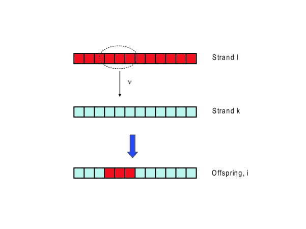
Figure 2: Pictorial representation of the horizontal gene transfer process considered.

Generalizing the method presented in Park and Deem (2007), we write the non-linear term as

$$\frac{\sum_{l}q_{l}R_{kl}^{i}}{\sum_{m}q_{m}}=\sum_{b=0}^{N/\bar{M}-1}\left\langle\prod_{j_{b}=\bar{M}b+1}^{\bar{M}(b+1)}\left(\frac{1+s_{j_{b}}^{l}s_{j_{b}}^{i}}{2}\right)\right\rangle\prod_{j\neq\{j_{b}\}}^{N}\left(\frac{1+s_{j}^{k}s_{j}^{i}}{2}\right).$$ (3)

Here, $\langle A_{l}\rangle=\sum_{l}q_{l}A_{l}/\sum_{m}q_{m}$ is a population average. At steady state, this average is independent of the value of $b$, due to the symmetry of the fitness function.

The variance of the composition $u^{l}=\frac{1}{N}\sum_{j=1}^{N}s_{j}^{l}$ is given by $\frac{1}{N^{2}}\sum_{j,j^{\prime}=1}^{N}\langle\delta s_{j}^{l}\delta s_{j^{\prime}}^{l}\rangle$. In the absence of recombination or horizontal gene transfer this variance is $\mathcal{O}(N^{-1})$, which implies correlations along the sequence are $\mathcal{O}(N^{-1})$ Park and Deem (2006). We expect the same scaling of the variance in the presence of recombination or horizontal gene transfer. Therefore, we introduce the factorization

$$\left\langle\prod_{j_{b}=\bar{M}b+1}^{\bar{M}(b+1)}\frac{1+s_{j_{b}}^{l}s_{j_{b}}^{i}}{2}\right\rangle \sim \prod_{j_{b}=\bar{M}b+1}^{\bar{M}(b+1)}\left\langle\frac{1+s_{j_{b}}^{l}s_{j_{b}}^{i}}{2}\right\rangle+\mathcal{O}(\bar{M}/N)$$

$$= \prod_{j_{b}=\bar{M}b+1}^{\bar{M}(b+1)}\left(\delta_{s_{j_{b}}^{i},+1}\frac{1+u(j_{b})}{2}+\delta_{s_{j_{b}}^{i},-1}\frac{1-u(j_{b})}{2}\right)$$

which becomes exact in the $N\rightarrow\infty$ limit. Here, $u(j_{b})=\sum_{l}q_{l}s_{j_{b}}^{l}/\sum_{m}q_{m}$ is the average base composition at site $j_{b}$.

We are interested in the long time behavior of the system, when the average base composition becomes independent of time and position $u(j)\sim u$. Thus, in the formalism of spin Boson operators Park and Deem (2007) $\vec{\hat{a}}(j)=(\hat{a}_{1}(j),\hat{a}_{2}(j))$, we define the recombination operator describing this recombination term by

$$\hat{R}=\frac{1}{N}\sum_{b=0}^{N/\bar{M}-1}\left[\prod_{j_{b}=\bar{M}b+1}^{\bar{M}(b+1)}[\rho_{+}\hat{a}_{1}^{\dagger}(j_{b})+\rho_{-}\hat{a}_{2}^{\dagger}(j_{b})][\hat{a}_{1}(j_{b})+\hat{a}_{2}(j_{b})]-\hat{I}\right]$$ (5)

Here, $\hat{I}$ is the identity operator. The coefficients $\rho_{\pm}=(1\pm u)/2$ represent Park and Deem (2007) the steady-state probability (per site) of having a “+1” or a “-1”. Defining the matrix

$$D=\left(\begin{array}[]{cc}\rho_{+}&\rho_{+}\\ \rho_{-}&\rho_{-}\end{array}\right),$$ (8)

the recombination operator in Eq. (5) can be expressed as

$$\hat{R}=\frac{1}{N}\sum_{b=0}^{N/\bar{M}-1}\left[\prod_{j_{b}=\bar{M}b+1}^{\bar{M}(b+1)}\vec{\hat{a}}^{\dagger}(j_{b})D\vec{\hat{a}}(j_{b})-\hat{I}\right].$$ (9)

II.1.1 The Hamiltonian

Considering the recombination operator in Eq. (9), we formulate the Hamiltonian describing the system

$$-\hat{H}=Nf\left[\frac{1}{N}\sum_{j=1}^{N}\vec{\hat{a}}^{\dagger}(j)\sigma_{3}\vec{\hat{a}}(j)\right]+\mu\sum_{j=1}^{N}[\vec{\hat{a}}^{\dagger}(j)\sigma_{1}\vec{\hat{a}}(j)-\hat{I}]+\nu\sum_{b=0}^{N/\bar{M}-1}\left[\prod_{j_{b}=\bar{M}b+1}^{\bar{M}(b+1)}\vec{\hat{a}}^{\dagger}(j_{b})D\vec{\hat{a}}(j_{b})-\hat{I}\right].$$ (10)

Here, $\sigma_{3}=\left(\begin{array}[]{cc}1&0\\ 0&-1\end{array}\right)$ and $\sigma_{1}=\left(\begin{array}[]{cc}0&1\\ 1&0\end{array}\right)$ are the Pauli matrices. We introduce a Trotter factorization

$$e^{-\hat{H}t}=\lim_{M\rightarrow\infty}\int\left[\mathcal{D}\vec{z}^{*}\mathcal{D}\vec{z}\right]|\vec{z}_{M}\rangle\left(\prod_{k=1}^{M}\langle\vec{z}_{k}|e^{-\epsilon\hat{H}}|\vec{z}_{k-1}\rangle\right)\langle\vec{z}_{0}|.$$ (11)

As shown in Appendix A, the partition function that gives the mean population fitness is

$$Z=\int\left[\mathcal{D}\bar{\xi}\mathcal{D}\xi\mathcal{D}\bar{\phi}\mathcal{D}\phi\right]e^{-S\left[\bar{\xi},\xi,\bar{\phi},\phi\right]}\sim e^{Nf_{m}t}.$$ (12)

Here, the action in the continuous time limit is

$$S\left[\bar{\xi},\xi,\bar{\phi},\phi\right] = -N\int_{0}^{t}dt\left[-\bar{\xi}\xi-\bar{\phi}\phi-\mu-\frac{\nu}{\bar{M}}+f(\xi)+\frac{\nu}{\bar{M}}\phi^{\bar{M}}\right]-N\ln Q.$$ (13)

II.1.2 The saddle point limit

In the $N\rightarrow\infty$ limit, the saddle point is exact and we obtain an analytical expression for the partition function Eq. (12). We look for the steady-state solution, when the fields become independent of time, $\xi_{c}$, $\bar{\xi}_{c}$, $\phi_{c}$, $\bar{\phi}_{c}$. The trace defined by Eq. (134) in the long time saddle-point limit becomes

$$\lim_{t\rightarrow\infty}\frac{\ln Q_{c}}{t}=\frac{\bar{\phi}_{c}}{2}+\left[\bar{\xi}_{c}(\bar{\xi}_{c}+u\bar{\phi}_{c})+(\mu+\bar{\phi}_{c}/2)^{2}\right]^{1/2}$$ (14)

Hence, the saddle-point action is

$$\lim_{N,t\rightarrow\infty}\frac{\ln Z}{Nt} = \lim_{t\rightarrow\infty}\frac{-S_{c}}{Nt}$$

$$=f_{m} = \max_{\xi_{c},\bar{\xi}_{c},\phi_{c},\bar{\phi}_{c}}\left\{f(\xi_{c})-\bar{\xi}_{c}\xi_{c}-\bar{\phi}_{c}\phi_{c}-\mu-\frac{\nu}{\bar{M}}+\frac{\nu}{\bar{M}}\phi_{c}^{\bar{M}}\right.$$ (15)

$$+\left.\frac{\bar{\phi}_{c}}{2}+\left[\bar{\xi}_{c}(\bar{\xi}_{c}+u\bar{\phi}_{c})+(\mu+\bar{\phi}_{c}/2)^{2}\right]^{1/2}\right\}.$$

As shown in Appendix B, the mean fitness of the population is

$$f_{m}=\max_{-1\leq\xi_{c}\leq 1}\bigg{\{}f(\xi_{c})-\mu-\frac{\nu}{\bar{M}}+\frac{\nu}{\bar{M}}[\phi_{c}(\xi_{c})]^{\bar{M}}+\mu\sqrt{1-\xi_{c}^{2}}\frac{\sqrt{1-u^{2}}(1+\frac{\nu}{2\mu}[\phi_{c}(\xi_{c})]^{\bar{M}-1})}{\left[\left(1+\frac{\nu}{2\mu}(1-u^{2})[\phi_{c}(\xi_{c})]^{\bar{M}-1}\right)^{2}-u^{2}\right]^{1/2}}\bigg{\}}.$$

(16)

Here, $\phi_{c}$ is given by Eq. (141), and the surplus $u$ is obtained through the self-consistency condition $f_{m}=f(u)$. Equation (16) represents an exact analytical expression for the mean fitness of an infinite population experiencing horizontal gene transfer. This expression is valid for an arbitrary, permutation invariant replication rate $f(u)$.

It is worth to notice that Eq. (16) is a natural generalization of the single-site horizontal gene transfer process described in Park and Deem (2007). Indeed, specializing the Eqs. (141) and (16) to the particular case $\bar{M}=1$, after some algebra, we obtain

$$f_{m}(\bar{M}=1)=\max_{-1\leq\xi_{c}\leq 1}\bigg{\{}f(\xi_{c})-\mu-\frac{\nu}{2}+\frac{\nu u}{2}\xi_{c}+\sqrt{1-\xi_{c}^{2}}\left[\left(\mu+\frac{\nu}{2}\right)^{2}-\left(\frac{u\nu}{2}\right)^{2}\right]^{1/2}\bigg{\}},$$ (17)

which reproduces the analytical result in Park and Deem (2007).

II.1.3 Numerical tests and examples

For numerical calculations, it is convenient to reformulate Eq. (1) in terms of the fraction of the population at a distance $l$ from the wild type, $P_{l}=\sum_{j\in\mathcal{C}_{l}}p_{j}$. Here, $\mathcal{C}_{l}$ is the class of sequences with $l$ number of “-1” sites. The number of sequences within this class is $\left(\begin{array}[]{c}N\\ l\end{array}\right)$.

As an example, for the case $\bar{M}=3$, the differential equation representing the time evolution of the probability distribution of classes within an infinite population of binary sequences is

$$\frac{dP_{l}}{dt} = N\left[f(2l/N-1)-\sum_{l^{\prime}=0}^{N}P_{l^{\prime}}f(2l^{\prime}/N-1)-\mu\right]P_{l}+\mu N\left[\frac{N-l+1}{N}P_{l-1}+\frac{l+1}{N}P_{l+1}\right]$$

$$+\frac{\nu}{3}N\left\{\rho_{-}^{3}g_{3}(N-l+3)P_{l-3}+[\rho_{-}^{3}h(N-l+2)+3\rho_{-}^{2}\rho_{+}g_{3}(N-l+2)]P_{l-2}\right.$$

$$+\left.[\rho_{-}^{3}h(l-1)+3\rho_{-}\rho_{+}^{2}g_{3}(N-l+1)+3\rho_{-}^{2}\rho_{+}h(N-l+1)]P_{l-1}\right.$$

$$+\left.[\rho_{+}^{3}h(N-l-1)+3\rho_{-}^{2}\rho_{+}g_{3}(l+1)+3\rho_{-}\rho_{+}^{2}h(l+1)]P_{l+1}\right.$$

$$+\left.[\rho_{+}^{3}h(l+2)+3\rho_{-}\rho_{+}^{2}g_{3}(l+2)]P_{l+2}+\rho_{+}^{3}g_{3}(l+3)P_{l+3}\right\}$$

$$-\frac{\nu}{3}N\left\{(\rho_{-}^{3}+3\rho_{-}^{2}\rho_{+}+3\rho_{-}\rho_{+}^{2})g_{3}(N-l)+(\rho_{-}^{3}+3\rho_{-}^{2}\rho_{+}+\rho_{+}^{3})h(N-l)\right.$$

$$+\left.(\rho_{-}^{3}+3\rho_{-}\rho_{+}^{2}+\rho_{+}^{3})h(l)+(\rho_{+}^{3}+3\rho_{+}\rho_{-}^{2}+3\rho_{-}\rho_{+}^{2})g_{3}(l)\right\}P_{l}$$

(18)

In writing this equation we have made use of the only $\mathcal{O}(N^{-1})$ correlations between sites, which holds at long time as well as for short time with suitable initial conditions. Here, we defined

$$\rho_{\pm}=\frac{1\pm u}{2}$$ (19)

where the average composition is calculated as

$$u=\sum_{l=0}^{N}\frac{N-2l}{N}P_{l}$$ (20)

and the functions

$$g_{3}(l) = \frac{l(l-1)(l-2)}{N(N-1)(N-2)}$$

$$h(l) = 3\frac{l(l-1)(N-l)}{N(N-1)(N-2)}$$ (21)

A comparison between the analytical expression Eq. (16) and the direct numerical solution of the differential Eq. (18) for N = 1002 is presented in Table 1, where the quadratic fitness $f(u)=ku^{2}/2$ was considered. We notice that the analytical method and the numerical solution provide the same results within $\mathcal{O}(N^{-1})$, as expected from the saddle point limit.

Table 1: Analytical versus numerical results for horizontal gene transfer in the parallel (Kimura) model for the quadratic fitness $f(u)=ku^{2}/2$, with $\bar{M}=3$.

$k/\mu$	$\nu/\mu$	$u^{\rm{numeric}}$	$u^{\rm{analytic}}$
2.0	0.0	0.4993	0.5000
2.0	0.5	0.4830	0.4838
2.0	1.0	0.4668	0.4677
2.0	1.5	0.4510	0.4519
2.5	0.0	0.5995	0.6000
2.5	0.5	0.5915	0.5920
2.5	1.0	0.5838	0.5844
2.5	1.5	0.5766	0.5772
5.0	0.0	0.7998	0.8000
5.0	0.5	0.7988	0.7990
5.0	1.0	0.7979	0.7981
5.0	1.5	0.7970	0.7972

The differential equation representing the horizontal gene transfer of blocks of size $\bar{M}=4$ within an infinite population of binary sequences is given by

$$\frac{d}{dt}P_{l} = N\left[f(2l/N-1)-\sum_{l^{\prime}=0}^{N}P_{l^{\prime}}f(2l^{\prime}/N-1)-\mu\right]P_{l}+\mu N\left[\frac{N-l+1}{N}P_{l-1}+\frac{l+1}{N}P_{l+1}\right]$$ (22)

$$+\frac{\nu}{4}N\left\{g_{4}(N-l+4)\rho_{-}^{4}P_{l-4}+[\rho_{-}^{4}h_{3}(N-l+3)+4\rho_{-}^{3}\rho_{+}g_{4}(N-l+3)]P_{l-3}\right.$$

$$+\left.[\rho_{-}^{4}h_{2}(l-2)+4\rho_{-}^{3}\rho_{+}h_{3}(N-l+2)\right.$$

$$+\left.6\rho_{-}^{2}\rho_{+}^{2}g_{4}(N-l+2)]P_{l-2}+[\rho_{-}^{4}h_{3}(l-1)+4\rho_{-}^{3}\rho_{+}h_{2}(l-1)\right.$$

$$+\left.6\rho_{-}^{2}\rho_{+}^{2}h_{3}(N-l+1)+4\rho_{-}\rho_{+}^{3}g_{4}(N-l+1)]P_{l-1}\right.$$

$$+\left.[\rho_{+}^{4}h_{3}(N-l-1)+4\rho_{-}\rho_{+}^{3}h_{2}(l+1)+6\rho_{-}^{2}\rho_{+}^{2}h_{3}(l+1)+4\rho_{-}^{3}\rho_{+}g_{4}(l+1)]P_{l+1}\right.$$

$$+\left.[\rho_{+}^{4}h_{2}(l+2)+4\rho_{-}\rho_{+}^{3}h_{3}(l+2)+6\rho_{-}^{2}\rho_{+}^{2}g_{4}(l+2)]P_{l+2}\right.$$

$$+\left.[\rho_{+}^{4}h_{3}(l+3)+4\rho_{-}\rho_{+}^{3}g_{4}(l+3)]P_{l+3}+\rho_{+}^{4}g_{4}(l+4)P_{l+4}\right\}$$

$$-\frac{\nu}{4}N\left\{[\rho_{-}^{4}+6\rho_{-}^{2}\rho_{+}^{2}+4\rho_{-}^{3}\rho_{+}+\rho_{+}^{4}]h_{3}(N-l)+[\rho_{-}^{4}+6\rho_{-}^{2}\rho_{+}^{2}+4\rho_{-}\rho_{+}^{3}+\rho_{+}^{4}]h_{3}(l)\right.$$

$$+\left.[4\rho_{-}^{3}\rho_{+}+6\rho_{-}^{2}\rho_{+}^{2}+4\rho_{-}\rho_{+}^{3}+\rho_{-}^{4}]g_{4}(N-l)+[4\rho_{-}^{3}\rho_{+}+6\rho_{-}^{2}\rho_{+}^{2}+4\rho_{-}\rho_{+}^{3}+\rho_{+}^{4}]g_{4}(l)\right.$$

$$+\left.[\rho_{-}^{4}+4\rho_{-}^{3}\rho_{+}+4\rho_{-}\rho_{+}^{3}+\rho_{+}^{4}]h_{2}(l)\right\}P_{l}$$

Here, the parameters $\rho_{\pm}$ and $u$ are defined, as before, by Eq. (19) and Eq. (20), respectively. We also define the functions

$$g_{4}(l) = \frac{l(l-1)(l-2)(l-3)}{N(N-1)(N-2)(N-3)}$$

$$h_{3}(l) = 4\frac{l(l-1)(l-2)(N-l)}{N(N-1)(N-2)(N-3)}$$

$$h_{2}(l) = 6\frac{l(l-1)(N-l)(N-l-1)}{N(N-1)(N-2)(N-3)}$$ (23)

A comparison between the analytical expression Eq. (16) and the direct numerical solution of the differential Eq. (22) for N = 1002 is presented in Table 2, for the quadratic fitness $f(u)=ku^{2}/2$. As in the former case, the numerical and analytical results agree to within $\mathcal{O}(N^{-1})$, as expected.

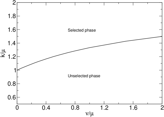
Figure 3: Phase diagram of the parallel (Kimura) model for the quadratic fitness $f(u)=ku^{2}/2$, with horizontal gene transfer of non-overlapping blocks of size $\bar{M}$. The phase boundary of the error threshold phase transition is given by the curve, and its shape is independent of the block size $\bar{M}$. In the absence of horizontal gene transfer, the phase transition occurs at $k/\mu=1$.

Table 2: Analytical versus numerical results for horizontal gene transfer in the parallel model for the quadratic fitness $f(u)=ku^{2}/2$, with $\bar{M}=4$.

$k/\mu$	$\nu/\mu$	$u^{\rm{numeric}}$	$u^{\rm{analytic}}$
2.0	0.0	0.4993	0.5000
2.0	0.5	0.4832	0.4840
2.0	1.0	0.4672	0.4680
2.0	1.5	0.4510	0.4519
2.5	0.0	0.5995	0.6000
2.5	0.5	0.5916	0.5921
2.5	1.0	0.5839	0.5845
2.5	1.5	0.5766	0.5773
5.0	0.0	0.7998	0.8000
5.0	0.5	0.7988	0.7990
5.0	1.0	0.7979	0.7981
5.0	1.5	0.7970	0.7973

For the quadratic fitness case in the absence of recombination ($\nu=0$), the exact analytical result predicts the existence of a “selected” organized phase, or quasi-species, when $k>\mu$. In this phase, the average composition is given by $u=1-\mu/k$. For $k<\mu$, a phase transition occurs and the quasi-species disappears in favor of a disordered or “unselected” phase with $u=0$. In Figure 3, we display the phase structure in the presence of horizontal gene transfer. In agreement with the numerical results presented in Table 1 and Table 2, the recombination scheme considered in this model introduces a mild mutational load. However, near the critical region $k/\mu\sim 1$, one observes that horizontal gene transfer distorts the phase boundary which defines the error threshold, from the horizontal line $k/\mu=1$, to a monotonically increasing curve that saturates for large values of $\nu/\mu$. We obtain an analytical expression for the phase boundary, by expanding Eqs. (141) and (16) near the critical region $\xi_{c}\sim 0$, $u\sim 0$. We find that the boundary is defined by

$$k_{\rm{crit}}=\mu\frac{1+\nu/\mu}{1+\nu/2\mu}.$$ (24)

We notice from this expression that for small $\nu$, $k_{\rm{crit}}\sim\mu+\nu/2$, whereas for large $\nu$ the phase boundary becomes asymptotically independent of $\nu$, $k_{\rm{crit}}\sim 2\mu$. We also notice from this formula that the phase boundary is independent of the block size $\bar{M}$.

As a second example, we consider a square-root fitness function

$$f(u)=k\sqrt{|u|}$$ (25)

In Table 3, we present a comparison of our analytical result, obtained from Eq. (16), with the direct numerical solution of the differential Eq. (18), for $\bar{M}=3$. As in the quadratic fitness example, the analytical and numerical results agree to order $\mathcal{O}(N^{-1})$, as expected.

Table 3: Analytical versus numerical results for horizontal gene transfer in the parallel (Kimura) model for the square-root fitness $f(u)=k\sqrt{|u|}$, with $\bar{M}=3$, N = 801.

$k/\mu$	$\nu/\mu$	$u^{\rm{numeric}}$	$u^{\rm{analytic}}$
2.0	0.0	0.4858	0.4855
2.0	0.5	0.4892	0.4889
2.0	1.0	0.4918	0.4915
2.0	1.5	0.4939	0.4936
2.5	0.0	0.5399	0.5396
2.5	0.5	0.5428	0.5425
2.5	1.0	0.5450	0.5448
2.5	1.5	0.5469	0.5466
4.0	0.0	0.6525	0.6523
4.0	0.5	0.6542	0.6540
4.0	1.0	0.6556	0.6554
4.0	1.5	0.6568	0.6565

From the results presented in Table 3, it is remarkable that the average composition $u$, and correspondingly the mean fitness of the population $f_{m}=k\sqrt{|u|}$, increase when increasing the horizontal gene transfer rate $\nu$.

The mutational deterministic hypothesis states that recombination is beneficial for negative epistasis fitness functions (see Fig. 1) $f^{{}^{\prime\prime}}(u)<0$, and deleterious for positive epistasis fitness functions, $f^{{}^{\prime\prime}}(u)>0$ Kimura and Maruyama (1966); Arjan et al. (2007); Azevedo et al. (2006); Kondrashov (1982, 1988, 1993). Our results for the quadratic and square-root fitness functions, Eqs. (16)–(24) and Tables 1, 2, and 3 provide support for this hypothesis. In fact, we can prove the mutational deterministic hypothesis holds for the parallel model in the presence of horizontal gene transfer, Appendix L.

Horizontal gene transfer has less of an effect for the sharp peak fitness, $f(u)=A\delta_{u,1}$. For general $\bar{M}$, the maximum in Eq. (16) is achieved for $\xi_{c}=1$, with $\phi_{c}(1)=(1+u)/2$ from Eq. (141). Thus, one obtains

$$f_{m}=A-\mu-\frac{\nu}{\bar{M}}\left[1-\left(\frac{1+u}{2}\right)^{\bar{M}}\right].$$ (26)

The error threshold is given for $u=0$ by the condition $A>\mu+\frac{\nu}{\bar{M}}(1-2^{-\bar{M}})$. However, we notice from Eq. (26) that $f_{m}(u=1)=A-\mu>f_{m}(u=0)$. Therefore, we have $u=1-\mathcal{O}(N^{-1})$ in the selected phase, with the effect of horizontal gene transfer being negligible for finite $\bar{M}$. We obtain the fraction of the population located at the peak $P_{0}$, from the self-consistency condition $P_{0}A=f_{m}$, which yields $P_{0}=1-\mu/A$. Thus, the true error threshold is at $A_{\rm{crit}}=\mu$, with the condition $A>\mu+\frac{\nu}{\bar{M}}(1-2^{-\bar{M}})$ defining the limit of metastability for initial conditions with $u\sim 0$. These results are similar to the ones obtained in the absence of horizontal gene transfer Park and Deem (2006, 2007); not (a). Thus, we conclude that for the sharp peak fitness, horizontal gene transfer does not spread out the population in sequence space. This result differs from the numerical studies presented in Boerlijst et al. (1996), where a mathematical model for ’uniform crossover’ recombination between viral strains super-infecting a population of cells was described. We remark that this model studied sequences of finite length (N = 15), where the error threshold transition is not really sharp. Our results correspond to the more realistic limit $N\rightarrow\infty$ (typical viral genomes are $10^{3}-10^{4}$).

In summary, from our exact analytical formula for the mean fitness Eq. (16), which is valid for any permutation invariant replication rate, we developed the explicit solution of three different examples: a quadratic fitness, a square-root fitness and a single sharp peak. For the case of smooth fitness functions, from our exact analytical formulas for the mean fitness $f_{m}$ and average composition $u$, we conclude that in agreement with the mutational deterministic hypothesis Kimura and Maruyama (1966); Arjan et al. (2007); Kondrashov (1982, 1988, 1993), a population whose fitness represents positive epistasis (i.e. quadratic), will experience an additional load against selection due to horizontal gene transfer. On the contrary, when negative epistasis is present (e.g. square-root), horizontal gene transfer is beneficial by enhancing selection. We provided a mathematical proof for this effect, Appendix L. When the fitness is defined by a single sharp peak, the population steady-state distribution behaves more rigidly in response to horizontal gene transfer. This fundamental difference can be attributed to the structure of the quasi-species distribution, which in the smooth fitness case is a Gaussian centered at the mean fitness, while in the sharp peak it is a fast decaying exponential, sharply peaked at the master sequence Park and Deem (2006). While the Gaussian distribution spreads its tails over a wide region of sequence space, thus allowing for horizontal gene transfer effects to propagate over a large diversity of mutants, the sharp exponential distribution concentrates in a narrow neighborhood of the master sequence, acting as a barrier to the propagation of such effects.

II.2 Horizontal gene transfer for multiple-size blocks

A natural extension to the model of horizontal gene transfer involving blocks of genes of a given size is to consider a process where each site along the sequence may be transferred with probability $\gamma$, or left intact with probability $1-\gamma$. The operator describing this process is

$$\hat{R}=\frac{1}{\langle\bar{M}\rangle}\prod_{j=1}^{N}\left[(1-\gamma)\hat{I}_{j}+\gamma\hat{R}_{j}\right]-\frac{1}{\langle\bar{M}\rangle}\hat{I}.$$ (27)

Here, $\hat{R}_{j}=\vec{\hat{a}}^{\dagger}(j)D\vec{\hat{a}}(j)$ is the single-site recombination operator defined in Eq. (5), with the matrix $D$ defined as in Eq. (8). Notice that this operator represents a binomial process, where an average number of sites $\langle\bar{M}\rangle=\gamma N$ is transferred. If we consider, as in the former finite block size case, that $N/\langle\bar{M}\rangle=\mathcal{O}(N)$, then we have $\gamma=\langle\bar{M}\rangle/N$, and for very large $N$ Eq. (27) reduces to

$$\hat{R}=\frac{1}{\langle\bar{M}\rangle}\prod_{j=1}^{N}\left[(1-\gamma)\hat{I}_{j}+\gamma\hat{R}_{j}\right]-\frac{1}{\langle\bar{M}\rangle}\hat{I}\sim\frac{1}{\langle\bar{M}\rangle}e^{-\langle\bar{M}\rangle+\frac{\langle\bar{M}\rangle}{N}\sum_{j=1}^{N}\vec{\hat{a}}^{\dagger}(j)D\vec{\hat{a}}(j)}-\frac{1}{\langle\bar{M}\rangle}\hat{I}.$$ (28)

Considering the recombination operator defined in Eq. (28), the spin Boson Hamiltonian for the Kimura model becomes

$$-\hat{H} = Nf\left[\frac{1}{N}\sum_{j=1}^{N}\vec{\hat{a}}^{\dagger}(j)\sigma_{3}\vec{\hat{a}}(j)\right]+\mu\sum_{j=1}^{N}[\vec{\hat{a}}(j)^{\dagger}\sigma_{1}\vec{\hat{a}}(j)-\hat{I}]+\frac{\nu}{\langle\bar{M}\rangle}Ne^{-\langle\bar{M}\rangle+\frac{\langle\bar{M}\rangle}{N}\sum_{j=1}^{N}\vec{\hat{a}}^{\dagger}(j)D\vec{\hat{a}}(j)}$$ (29)

$$-\frac{\nu}{\langle\bar{M}\rangle}N\hat{I}.$$

We introduce a Trotter factorization

$$e^{-\hat{H}t}=\lim_{M\rightarrow\infty}\int\left[\mathcal{D}\vec{z}^{*}\mathcal{D}\vec{z}\right]|\vec{z}_{M}\rangle\left(\prod_{k=1}^{M}\langle\vec{z}_{k}|e^{-\epsilon\hat{H}}|\vec{z}_{k-1}\rangle\right)\langle\vec{z}_{0}|.$$ (30)

As shown in Appendix C, the partition function becomes

$$Z=\int\left[\mathcal{D}\bar{\xi}\mathcal{D}\xi\mathcal{D}\bar{\phi}\mathcal{D}\phi\right]e^{-S\left[\bar{\xi},\xi,\bar{\phi},\phi\right]}\sim e^{Nf_{m}t}.$$ (31)

Here, the action in the continuous time limit is

$$S\left[\bar{\xi},\xi,\bar{\phi},\phi\right]=-N\int_{0}^{t}dt^{\prime}\left[-\bar{\xi}\xi-\bar{\phi}\phi-\mu-\frac{\nu}{\langle\bar{M}\rangle}+f(\xi)+\frac{\nu}{\langle\bar{M}\rangle}e^{-\langle\bar{M}\rangle(1-\phi)}\right]-N\ln Q$$ (32)

II.2.1 The saddle point limit

As in the previous model, the saddle point limit is exact as $N\rightarrow\infty$ in Eq. (32).

After a similar procedure as in section II.A.2, we find the saddle-point equation for the mean fitness

$$f_{m} = \max_{-1\leq\xi_{c}\leq 1}\Biggl{\{}f(\xi_{c})-\mu-\frac{\nu}{\langle\bar{M}\rangle}+\frac{\nu}{\langle\bar{M}\rangle}e^{-\langle\bar{M}\rangle(1-\phi_{c}(\xi_{c}))}$$ (33)

$$~{}~{}~{}~{}~{}~{}~{}~{}~{}+\mu\sqrt{1-\xi_{c}^{2}}\frac{\sqrt{1-u^{2}}(1+\frac{\nu}{2\mu}e^{-\langle\bar{M}\rangle(1-\phi_{c}(\xi_{c}))})}{\left[\left(1+\frac{\nu}{2\mu}(1-u^{2})e^{-\langle\bar{M}\rangle(1-\phi_{c}(\xi_{c}))}\right)^{2}-u^{2}\right]^{1/2}}\Biggr{\}}$$

Here, $\phi_{c}(\xi_{c})$ is obtained from the equation

$$\phi_{c}(\xi_{c})=\frac{1+u\xi_{c}}{2}+\frac{\sqrt{1-\xi_{c}^{2}}}{2}\frac{\sqrt{1-u^{2}}}{\left[1-\left(\frac{u}{1+\frac{\nu}{2\mu}(1-u^{2})e^{-\langle\bar{M}\rangle(1-\phi_{c})}}\right)^{2}\right]^{1/2}}$$ (34)

Eq. (33) represents an exact analytical expression for the mean fitness $f_{m}$ of an infinite population experiencing horizontal gene transfer of multiple size sequences. The formula is valid for an arbitrary, permutation invariant replication rate function $f(u)$.

Table 4: Analytical results for horizontal gene transfer in the parallel model for the quadratic fitness $f(u)=\frac{k}{2}u^{2}$, with $\langle\bar{M}\rangle=3$.

$k$	$\nu$	$u^{\rm{analytic}}$
2.0	0.0	0.50
2.0	0.5	0.4840
2.0	1.0	0.4680
2.0	1.5	0.4522
2.5	0.0	0.6000
2.5	0.5	0.5921
2.5	1.0	0.5845
2.5	1.5	0.5773
4.0	0.0	0.8000
4.0	0.5	0.7990
4.0	1.0	0.7981
4.0	1.5	0.7973

We notice that recombination introduces an additional mutational load against selection. This load is mild at low values of the fitness constant $k$, and becomes negligibly small at larger values. Numerical evaluation of Eqs. (33) and (34) is presented in Table 4 for the quadratic fitness $f(u)=ku^{2}/2$, and average block size $\langle\bar{M}\rangle=3$.

An analytical expression for the phase boundary is obtained from Eqs. (33) and (34), near the error threshold $u\sim 0$, $\xi_{c}\sim 0$. We find

$$k_{\rm{crit}}=\mu\frac{1+\frac{\nu}{\mu}}{1+\frac{\nu}{2\mu}}$$ (35)

We notice that for small $\nu$, the critical value is $k_{\rm{crit}}\sim\mu+\nu/2$, whereas for large values of $\nu$ it becomes independent of recombination $k_{\rm{crit}}\sim 2\mu$. This behavior is similar to the one previously observed in Fig. 3 for the case of horizontal gene transfer with blocks of fixed size. The shape of the phase boundary is independent of the block size in the horizontal gene transfer process, assuming that the size of the blocks is finite.

As a second example, we consider the square root fitness $f(u)=k\sqrt{|u|}$. Analytical results for the average composition, obtained after Eq. (16), are represented in Table 5 for blocks of average size $\langle\bar{M}\rangle=3$.

Table 5: Analytical results for horizontal gene transfer in the parallel model for the square-root fitness $f(u)=k\sqrt{|u|}$, with $\langle\bar{M}\rangle=3$.

$k$	$\nu$	$u^{\rm{analytic}}$
2.0	0.0	0.4855
2.0	0.5	0.4889
2.0	1.0	0.4915
2.0	1.5	0.4936
2.5	0.0	0.5396
2.5	0.5	0.5425
2.5	1.0	0.5448
2.5	1.5	0.5466
5.0	0.0	0.6523
5.0	0.5	0.6540
5.0	1.0	0.6554
5.0	1.5	0.6566

From the values displayed in Table 5, we notice that horizontal gene transfer introduces a mild increase in the average composition and, correspondingly, in the mean fitness of the population $f_{m}=k\sqrt{|u|}$. This trend, which is opposite to the quadratic fitness case, can be attributed to the negative epistasis represented by the square root fitness, by similar arguments as in the case of fixed block size.

Horizontal gene transfer does not affect the phase boundary for the sharp peak fitness, $f(u)=A\delta_{u,1}$. In this case, Eq. (33) is maximized at $\xi_{c}=1$, with $\phi_{c}=(1+u)/2$ from Eq. (34). Thus, the mean fitness becomes

$$f_{m}=A-\mu-\frac{\nu}{\langle\bar{M}\rangle}[1-e^{-\langle\bar{M}\rangle(1-u)/2}]$$ (36)

The error threshold is given, for $u=0$ in Eq. (36), by the condition $A>\mu+\frac{\nu}{\langle\bar{M}\rangle}[1-e^{-\langle\bar{M}\rangle/2}]$. However, we notice that $f_{m}(u=1)=A-\mu>f_{m}(u=0)$. Hence, in the selected phase $u=1-\mathcal{O}(N^{-1})$, and the recombination effect becomes negligible for infinite N. From the self-consistency condition $f_{m}=P_{0}A$, we obtain the fraction of the population located at the peak $P_{0}=1-\mu/A$. Therefore, the true error threshold is given by $A_{\rm{crit}}>\mu$, with $A>\mu+\frac{\nu}{\langle\bar{M}\rangle}[1-e^{-\langle\bar{M}\rangle/2}]$ the limit of metastability for initial conditions with $u\sim 0$.

Therefore, we conclude that horizontal gene transfer for multiple size blocks displays a qualitatively similar behavior to the corresponding process for fixed block size. A population evolving under a smooth fitness function with positive epistasis (e.g. quadratic, see Fig. 1) experiences an additional mutational load due to horizontal gene transfer, which modifies the quasi-species structure, reducing the mean fitness, and hence shifting the error threshold. On the contrary, when epistasis is negative (e.g. square-root, see Fig. 1) a beneficial effect is induced by horizontal gene transfer, in agreement with the mutational deterministic hypothesis, as we demonstrate in Appendix L.

A discontinuous sharp peak fitness function does not change the quasi-species distribution or the mean fitness, although it does introduce metastability.

II.3 The parallel model with two-parent recombination

Biological recombination, as occurs for example in viral super- or co-infection or in sexual reproduction, involves the crossing over of parental strands at random points along the sequence. The copying process is carried out by the action of polymerase enzymes, which move alternatively along one or the other parental strand. An approximate representation of this process is to consider that the polymerase enzyme starts, with probability 1/2 on either parental strand, copying one base at a time. We consider the crossovers to occur because there exists a probability $p_{c}$ per site that the polymerase “jumps” from its current position towards the other parental strand. Alternatively, the enzyme progresses along the current strand with probability $1-p_{c}$. A pictorial representation is shown in Fig. 4.

For this particular process representing the wandering path followed by the polymerase enzyme, the recombination coefficients $R_{kl}^{i}$ in Eq. (1) are given by the exact analytical expression

$$R_{kl}^{i} = \frac{1}{2}\sum_{\{\alpha_{j}=\pm 1\}}\left(\frac{1+s_{1}^{k}s_{1}^{i}}{2}\right)^{\frac{1+\alpha_{1}}{2}}\left(\frac{1+s_{1}^{l}s_{1}^{i}}{2}\right)^{\frac{1-\alpha_{1}}{2}}$$

$$\times[(1-p_{c})^{\frac{1+\alpha_{1}\alpha_{2}}{2}}p_{c}^{\frac{1-\alpha_{1}\alpha_{2}}{2}}]\left(\frac{1+s_{2}^{k}s_{2}^{i}}{2}\right)^{\frac{1+\alpha_{2}}{2}}\left(\frac{1+s_{2}^{l}s_{2}^{i}}{2}\right)^{\frac{1-\alpha_{2}}{2}}$$

$$\times[(1-p_{c})^{\frac{1+\alpha_{2}\alpha_{3}}{2}}p_{c}^{\frac{1-\alpha_{2}\alpha_{3}}{2}}]\left(\frac{1+s_{3}^{k}s_{3}^{i}}{2}\right)^{\frac{1+\alpha_{3}}{2}}\left(\frac{1+s_{3}^{l}s_{3}^{i}}{2}\right)^{\frac{1-\alpha_{3}}{2}}$$

$$\times\ldots\times[(1-p_{c})^{\frac{1+\alpha_{N-1}\alpha_{N}}{2}}p_{c}^{\frac{1-\alpha_{N-1}\alpha_{N}}{2}}]\left(\frac{1+s_{N}^{k}s_{N}^{i}}{2}\right)^{\frac{1+\alpha_{N}}{2}}\left(\frac{1+s_{N}^{l}s_{N}^{i}}{2}\right)^{\frac{1-\alpha_{N}}{2}}$$

Here, the recombining parental sequences are $S_{k}=(s_{1}^{k},s_{2}^{k},\ldots,s_{N}^{k})$, $S_{l}=(s_{1}^{l},\ldots,s_{N}^{l})$ and the offspring sequence is $S_{i}=(s_{1}^{i},s_{2}^{i},\ldots,s_{N}^{i})$, with $s_{j}=\pm 1$.

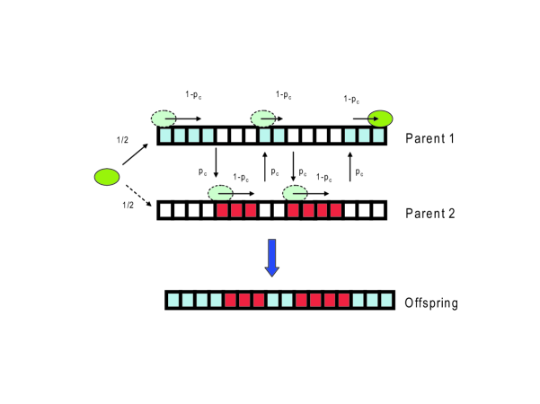
Figure 4: Pictorial representation of the two-parent genetic recombination process considered in the theory.

Using Eq. (LABEL:eq61), Eq. (1) representing the time evolution of an infinite population of binary sequences experiencing replication, point mutations and two-parent recombination, exactly becomes

$$\frac{dq_{i}}{dt} = r_{i}q_{i}+\sum_{k=1}^{2^{N}}\mu_{ik}q_{k}+\nu N\sum_{k=1}^{2^{N}}\frac{1}{2}\sum_{\{\alpha_{j}=\pm 1\}}\left\{\left[\prod_{j=2}^{N}p_{c}^{\frac{1-\alpha_{j-1}\alpha_{j}}{2}}(1-p_{c})^{\frac{1+\alpha_{j-1}\alpha_{j}}{2}}\right]\right.$$ (38)

$$\times\left.\prod_{j=1}^{N}\left(\frac{1+s_{j}^{k}s_{j}^{i}}{2}\right)^{\frac{1+\alpha_{j}}{2}}\sum_{l=1}^{2^{N}}p_{l}\left(\frac{1+s_{j}^{l}}{2}\delta_{s_{j}^{i},+1}+\frac{1-s_{j}^{l}}{2}\delta_{s_{j}^{i},-1}\right)^{\frac{1-\alpha_{j}}{2}}\right\}q_{k}-\nu Nq_{i}$$

where, again, $p_{l}=q_{l}/\sum_{l=1}^{2^{N}}q_{l}$ is the normalized probability for sequence $1\leq l\leq 2^{N}$.

From Eq. (38), the recombination operator corresponding to this recombination process in the spin Boson representation is

$$\hat{R} = \frac{1}{2}\sum_{l=1}^{2^{N}}p_{l}\sum_{\{\alpha_{i}=\pm 1\}}[\hat{I}_{1}^{\frac{1+\alpha_{1}}{2}}\hat{R}_{l}(1)^{\frac{1-\alpha_{1}}{2}}]\times[(1-p_{c})^{\frac{1+\alpha_{1}\alpha_{2}}{2}}p_{c}^{\frac{1-\alpha_{1}\alpha_{2}}{2}}]$$ (39)

$$\times[\hat{I}_{2}^{\frac{1+\alpha_{2}}{2}}\hat{R}_{l}(2)^{\frac{1-\alpha_{2}}{2}}]\times[(1-p_{c})^{\frac{1+\alpha_{2}\alpha_{3}}{2}}p_{c}^{\frac{1-\alpha_{2}\alpha_{3}}{2}}]\times[\hat{I}_{3}^{\frac{1+\alpha_{3}}{2}}\hat{R}_{l}(3)^{\frac{1-\alpha_{3}}{2}}]$$

$$\times\ldots\times[(1-p_{c})^{\frac{1+\alpha_{N-1}\alpha_{N}}{2}}p_{c}^{\frac{1-\alpha_{N-1}\alpha_{N}}{2}}]\times[\hat{I}_{N}^{\frac{1+\alpha_{N}}{2}}\hat{R}_{l}(N)^{\frac{1-\alpha_{N}}{2}}]-\hat{I}$$

$$\equiv g(\{\hat{R}_{l}(j)\})-\hat{I}$$

Here, the local recombination operator is $\hat{R}_{l}(j)=\vec{\hat{a}}(j)^{\dagger}D_{j}^{l}\vec{\hat{a}}(j)$, with

$$D_{j}^{l}=\left(\begin{array}[]{cc}\frac{1+s_{j}^{l}}{2}&\frac{1+s_{j}^{l}}{2}\\ \frac{1-s_{j}^{l}}{2}&\frac{1-s_{j}^{l}}{2}\end{array}\right).$$ (42)

The $\hat{I}_{j}$ are the identity operators acting on site $1\leq j\leq N$, whereas $\hat{I}=\prod_{j=1}^{N}\hat{I}_{j}$ is the identity operator for the entire sequence vector.

II.3.1 The Hamiltonian

The Hamiltonian describing the evolution of this system in the spin Boson representation is given by

$$-\hat{H}=Nf\left[\frac{1}{N}\sum_{j=1}^{N}\vec{\hat{a}}^{\dagger}(j)\sigma_{3}\vec{\hat{a}}(j)\right]+\mu\sum_{j=1}^{N}\left[\vec{\hat{a}}^{\dagger}(j)\sigma_{1}\vec{\hat{a}}(j)-\hat{I}\right]+\nu N\left(g[\{\hat{R}_{l}(j)\}]-\hat{I}\right)$$ (43)

We introduce a Trotter factorization

$$e^{-\hat{H}t}=\lim_{M\rightarrow\infty}\int\left[\mathcal{D}\vec{z}^{*}\mathcal{D}\vec{z}\right]|\vec{z}_{M}\rangle\left(\prod_{k=1}^{M}\langle\vec{z}_{k}|e^{-\epsilon\hat{H}}|\vec{z}_{k-1}\rangle\right)\langle\vec{z}_{0}|$$ (44)

As shown in Appendix D the partition function is

$$Z=\int\left[\mathcal{D}\bar{\xi}\mathcal{D}\xi\mathcal{D}\bar{\phi}\mathcal{D}\phi\right]e^{-S\left[\bar{\xi},\xi,\bar{\phi},\phi\right]}$$ (45)

Here, the action in the continuous time limit is given by

$$S\left[\bar{\xi},\xi,\bar{\phi},\phi\right]=-N\int_{0}^{t}dt\left[-\bar{\xi}\xi-\bar{\phi}\phi-\mu-\nu+f(\xi)+\nu g(\phi)\right]-N\ln Q$$ (46)

As shown in Appendix E, the recombination term can be represented, for $0\leq p_{c}\leq 1/2$, by the exact finite series

$$g(\{\psi_{j}^{l}\}) = \sum_{l=1}^{2^{N}}p_{l}\left\{\prod_{j=1}^{N}\left(\frac{1+\psi_{j}^{l}}{2}\right)\right.$$

$$+\left.\sum_{1\leq i<j}^{N}(1-2p_{c})^{j-i}\frac{1-\psi_{j}^{l}}{2}\frac{1-\psi_{i}^{l}}{2}\prod_{k\neq i,j}^{N}\left(\frac{1+\psi_{k}^{l}}{2}\right)\right.$$

$$+\left.\sum_{1\leq i<j<k<n}^{N}(1-2p_{c})^{j-i+n-k}\frac{1-\psi_{j}^{l}}{2}\frac{1-\psi_{i}^{l}}{2}\frac{1-\psi_{n}^{l}}{2}\frac{1-\psi_{k}^{l}}{2}\right.$$

$$\times\left.\prod_{m\neq i,j,k,n}^{N}\left(\frac{1+\psi_{m}^{l}}{2}\right)+\ldots+(1-2p_{c})^{\lfloor\frac{N}{2}\rfloor}\prod_{j=1}^{N}\left(\frac{1-\psi_{j}^{l}}{2}\right)\right\}$$

were we used the notation $\psi_{j}^{l}=\vec{z}^{*}_{k}(j)D_{j}^{l}\vec{z}_{k-1}(j)$, and $D_{j}^{l}$ is defined in Eq. (42).

We consider first the case when $p_{c}=1/2$ in the above expression. Then, we have

$$g(\{\psi_{j}^{l}\},p_{c}=1/2)=\sum_{l=1}^{2^{N}}p_{l}\prod_{j=1}^{N}(1+\psi_{j}^{l})/2$$ (48)

We notice that the recombination term in the differential Eq. (38) satisfies $\sum_{l=1}^{2^{N}}p_{l}R_{kl}^{i}\leq 1,\>\forall\>k,i$, because $R_{kl}^{i}\geq 0$ and $\sum_{i=1}^{2^{N}}R_{kl}^{i}=1$. In our field theoretic representation of the model, this condition is equivalent to $g(\{\psi_{j}^{l}\})\leq 1$ for any physical state. We also have, for example, $\left\langle\prod_{j=1}^{N}\left(\frac{1+\psi_{j}^{l}}{2}\right)\right\rangle_{z}\leq 1$. If we consider evaluating the $g$ interaction term perturbatively, as in Appendix A, we obtain terms such as

$$\langle g\rangle = [(1+\langle\psi\rangle)/2]^{N}+[(1+\langle\psi\rangle)/2]^{N-2}$$ (49)

$$\times(1/8)\sum_{l}p_{l}\sum_{i\neq j}\langle\delta\psi_{i}^{l}\delta\psi_{j}^{l}\rangle_{z}+\ldots$$

where $\langle\psi\rangle=\sum_{l}p_{l}(1/N)\sum_{j}\langle\psi_{j}^{l}\rangle_{z}$. Since both the correlations of the spins in the $D_{i}^{l}$ matrix for typical, likely $l$ and the correlations in the $z$ fields are each $\mathcal{O}(1/N)$, the interaction term $g$ in Eq. (48) contributes nothing, unless $\langle\psi\rangle=1-\mathcal{O}(1/N)$, in which case $\langle g\rangle=\mathcal{O}(N^{0})$.

For the general case of $0<p_{c}<1/2$, we notice that $0<1-2p_{c}<1$. Making the ansatz that correlations between $z$ fields and correlations between spins of typical, likely sequences $l$ each remain $\mathcal{O}(1/N)$ at different sites, terms other than the first in Eq. (LABEL:eq70) are at least $\mathcal{O}(1/N)$ smaller when $\langle\psi\rangle=1-\mathcal{O}(1/N)$. Thus, when $\langle\psi\rangle\sim 1$, the first term dominates the series, and the others become arbitrarily small, thus recovering the same expression as for $p_{c}=1/2$. On the other hand, when $\langle\psi\rangle\sim-1$, we notice that the dominant terms are the last ones. However, those terms are proportional to powers of $1-2p_{c}$ of order $N$, whereas the number of these terms is of just polynomial order in $N$. Therefore, for N very large these terms become arbitrary small. Thus, we conclude that in the limit $N\rightarrow\infty$, regardless of the value of $p_{c}$, the function $g$ is represented by Eq. (48).

In the particular case of uniform crossover $p_{c}=1/2$, and when the fitness function is permutation invariant, i.e., it depends only on the average composition of the sequence through the average base composition $u$, it is possible to reformulate the differential equation Eq. (1) for the evolutionary dynamics of an infinite population of binary sequences in terms of the distribution of classes:

$$P_{l}=\sum_{j\in\mathcal{C}_{l}}p_{j}$$ (50)

where $\mathcal{C}_{l}$ represents the class of sequences with $l$, “$-1$” spins. Although all the sequences in a given class do not have the same dynamics, we can nonetheless calculate the class dynamics exactly:

$$\frac{dP_{l}}{dt} = N\left[f(2l/N-1)-\sum_{l^{\prime}=0}^{N}P_{l^{\prime}}f(2l^{\prime}/N-1)\right]P_{l}+\mu(N-l+1)P_{l-1}+\mu(l+1)P_{l+1}-N\mu P_{l}$$ (51)

$$+\nu N\sum_{l_{1},l_{2}}R(l|l_{1},l_{2})P_{l_{1}}P_{l_{2}}-N\nu P_{l}.$$

The coefficients $R(l|l_{1},l_{2})$ represent the probability that a pair of parental sequences in the classes $\mathcal{C}_{l_{1}}$, $\mathcal{C}_{l_{2}}$, due to uniform crossover recombination, generate a child sequence in the class $\mathcal{C}_{l}$. The number of sequences in these classes is $\left(\begin{array}[]{c}N\\ l_{1}\end{array}\right)$, $\left(\begin{array}[]{c}N\\ l_{2}\end{array}\right)$ and $\left(\begin{array}[]{c}N\\ l\end{array}\right)$, respectively. For a given pair of parental sequences, let us consider the variables $n_{++}$, $n_{+-}$, $n_{-+}$ and $n_{--}$, representing the number of pairs of $(+1,+1)$, $(+1,-1)$, $(-1,+1)$ and $(-1,-1)$ spins respectively. These variables satisfy the equation $N=n_{++}+n_{+-}+n_{-+}+n_{--}$. We further notice that these variables also satisfy $n_{-+}=l_{1}-n_{--}$ and $n_{+-}=l_{2}-n_{--}$. Considering that from each pair of $(+1,-1)$ or $(-1,+1)$ spins in the parental sequences, the child sequence will inherit a “-1” spin with probability $1/2$, while from a pair of the kind $(-1,-1)$ it will inherit a “-1” spin with probability $1$, we have the explicit analytical expression for these coefficients

$$R(l|l_{1},l_{2})=\sum_{n=\max{\{0,l_{1}+l_{2}-N\}}}^{\min{\{l_{1}+l_{2}-l,l_{1},l_{2}\}}}\frac{\binom{N}{n,l_{1}-n,l_{2}-n}}{\binom{N}{l_{1}}\binom{N}{l_{2}}}\binom{l_{1}+l_{2}-2n}{l-n}2^{-(l_{1}+l_{2}-2n)}$$

(52)

The first factor is the probability for a configuration with $n\equiv n_{--}$, given $l_{1}$, $l_{2}$ and $l$. The second factor is the number of ways of picking $l-n_{--}$ “-1” spins among $n_{+-}+n_{-+}$. The third factor is just $(1/2)^{n_{-+}}(1/2)^{n_{+-}}(1)^{n_{--}}$. These coefficients are different from zero only if

$$\max{\{0,l_{1}+l_{2}-N\}\leq l\leq\min{\{N,l_{1}+l_{2}\}}}$$ (53)

They also satisfy the following properties:

$$R(l|l_{1},l_{2})=R(l|l_{2},l_{1})$$ (54)

$$\sum_{l=0}^{N}R(l|l_{1},l_{2})=1 \forall~{}l_{1},l_{2}$$ (55)

$$R(N|N,N)=R(0|0,0)=1$$ (56)

In the limit of large $N$, we find that the recombination coefficients satisfy a Gaussian distribution in the variables $u_{1}=1-2l_{1}/N$, $u_{2}=1-2l_{2}/N$, and $u=1-2l/N$ (see Appendix F):

$$R_{u_{1},u_{2}}^{u}\sim\frac{e^{-N\left[(u_{1}+u_{2})/2-u\right]^{2}/(1-u_{*}^{2})}}{\sqrt{\pi(1-u_{*}^{2})/N}}$$ (57)

where $f_{m}=f(u_{*})$.

This form of the recombination operator, Eq. (57), is equivalent to Eq. (48) with $s_{j}^{l}$ replaced by $u$ in the $D$ matrix. Alternatively, we notice that when the singular behavior of the function $g$ can be described as a delta function, we have

$$g = \sum_{l=1}^{2^{N}}p_{l}\delta_{\frac{1}{N}\sum_{j=1}^{N}\vec{z}_{k}^{*}(j)D_{j}^{l}\vec{z}_{k-1}(j),1}$$ (58)

$$= \sum_{l=1}^{2^{N}}p_{l}\int_{0}^{2\pi}\frac{d\lambda}{2\pi}e^{i\lambda\left[\frac{1}{N}\sum_{j=1}^{N}\vec{z}_{k}^{*}(j)D_{j}^{l}\vec{z}_{k-1}(j)-1\right]}$$

$$= \sum_{l=1}^{2^{N}}p_{l}\int_{0}^{2\pi}\frac{d\lambda}{2\pi}e^{-i\lambda}\left\{1+\frac{i\lambda}{N}\sum_{j=1}^{N}\vec{z}_{k}^{*}(j)D_{j}^{l}\vec{z}_{k-1}(j)\right.$$

$$+\left.\frac{1}{2!}\left(\frac{i\lambda}{N}\right)^{2}\sum_{j,m=1}^{N}\vec{z}_{k}^{*}(j)D_{j}^{l}\vec{z}_{k-1}(j)\vec{z}^{*}_{k}(m)D_{m}^{l}\vec{z}_{k-1}(m)+\ldots\right\}$$

By noticing that correlations between compositions at different sites along the sequence are of order $\mathcal{O}(N^{-1})$, we have that for the second order correlation

$$\langle D_{j}^{l}D_{m}^{l}\rangle-\langle D_{j}^{l}\rangle^{2}\sim\mathcal{O}(N^{-1})$$ (59)

where $\langle D_{j}^{l}\rangle=\sum_{l=1}^{2^{N}}p_{l}D_{j}^{l}\equiv D_{j}$ is the population average. A similar analysis for the higher order correlations allows us to factorize order by order the terms in the series Eq. (58), to obtain

$$g\sim\delta_{\frac{1}{N}\sum_{j=1}^{N}\vec{z}_{k}^{*}(j)D_{j}\vec{z}_{k-1}(j),1}+\mathcal{O}(N^{-1})$$ (60)

We are interested in the long term, steady state distribution, when the average base composition $u(j)=\langle s_{j}^{l}\rangle\sim u$ becomes independent of time. In this limit, the trace defined by Eq. (170) becomes

$$\lim_{t\rightarrow\infty}\frac{\ln Q_{c}}{t}=\frac{\bar{\phi}_{c}}{2}+\left[\bar{\xi}_{c}(\bar{\xi}_{c}+u\bar{\phi}_{c})+(\mu+\bar{\phi}_{c}/2)^{2}\right]^{1/2}$$ (61)

Hence, from Eq. (46), the saddle point action is

$$\lim_{N,t\rightarrow\infty}\frac{\ln Z}{Nt} = \lim_{t\rightarrow\infty}\frac{-S_{c}}{Nt}=f_{m}$$ (62)

$$= \max_{\xi_{c},\bar{\xi}_{c},\phi_{c},\bar{\phi}_{c}}\bigg{\{}-\bar{\xi}_{c}\xi_{c}-\bar{\phi}_{c}\phi_{c}-\mu-\nu+\nu g(\phi_{c})$$

$$~{}~{}~{}~{}~{}~{}~{}~{}~{}~{}+f(\xi_{c})+\frac{\bar{\phi}_{c}}{2}+\left[\bar{\xi}_{c}(\bar{\xi}_{c}+u\bar{\phi}_{c})+\left(\mu+\frac{\bar{\phi}_{c}}{2}\right)^{2}\right]^{1/2}\bigg{\}}$$

As shown in Appendix G, we find

$$\frac{-S_{c}}{Nt} = \max_{\phi_{c},\xi_{c}}\left\{f(\xi_{c})-\mu-\nu+\nu g(\phi_{c})+\frac{\mu}{1-u^{2}}(2\phi_{c}-1-u\xi_{c})\right.$$ (63)

$$~{}~{}~{}~{}~{}~{}~{}~{}-\left.\frac{\mu|u|}{1-u^{2}}\left[(2\phi_{c}-1-u\xi_{c})^{2}-(1-u^{2})(1-\xi_{c}^{2})\right]^{1/2}\right\}$$

Because of the singular behavior of the function $g(\phi_{c})$, to find the saddle point we need to consider three separate cases: $\phi_{c}<1$, $\phi_{c}=1$, and $\phi_{c}=1-\mathcal{O}(1/N)$. The existence of different expressions for the mean fitness suggests the possibility of different selected phases in certain conditions. We also notice that the saddle point analysis may not apply exactly, unless $g(\phi_{c})=\delta_{\phi_{c},1}$.

Case 1: $\phi_{c}<1$. For this case, we look for a saddle point in the field $\phi_{c}$, in the interior of the domain, $\phi_{c}<1$ where $g(\phi_{c})=0$

$$\frac{\delta}{\delta\phi_{c}}\left(\frac{-S_{c}}{Nt}\right)=\frac{2\mu}{1-u^{2}}-\frac{\mu|u|}{1-u^{2}}\frac{2(2\phi_{c}-1-u\xi_{c})}{\left[(2\phi_{c}-1-u\xi_{c})^{2}-(1-u^{2})(1-\xi_{c}^{2})\right]^{1/2}}=0$$ (64)

From Eq. (64), we solve for $\phi_{c}$ as a function of $\xi_{c}$

$$\phi_{c}(\xi_{c})=\frac{1+u\xi_{c}}{2}+\frac{1}{2}\sqrt{1-\xi_{c}^{2}}$$ (65)

Substituting Eq. (65) in the saddle-point action Eq. (63), we obtain

$$f_{m}^{(1)}=\max_{-1\leq\xi_{c}\leq 1}\left\{f(\xi_{c})-\mu-\nu+\mu\sqrt{1-\xi_{c}^{2}}\right\}$$ (66)

Case 2: $\phi_{c}=1$. The mean fitness is obtained from Eq. (63) as

$$f_{m}^{(2)}=\max_{-1\leq\xi_{c}\leq 1}\{f(\xi_{c})-\mu+\frac{\mu}{1-u^{2}}(1-u\xi_{c}-|u\xi_{c}-u^{2}|)\}$$ (67)

Case 3: $\phi_{c}=1-\mathcal{O}(1/N)$. In this case, additional analysis is necessary to calculate the mean fitness due to the singular behavior of the $g(\phi_{c})$ function. For a smooth fitness function, we can argue this case does not exist. We first consider the Hamiltonian (43) for the case $g=0$. The largest eigenvalue, $f_{m}$, is shifted by $-\nu$ relative to the $\nu=0$ case. This allows us to calculate the average composition, $u_{*}$, from the implicit relation $f_{m}(\nu)=f_{m}(\nu=0)-\nu=f(u_{*})$. Alternatively, if we consider the differential equation for the unnormalized class probabilities, $dQ/dt=LQ$, we see that the differential operator $L$ looks like that in the absence of recombination, save for a shift of $-\nu$ in the fitness function. Thus, the variance of the population is given by Park and Deem (2006) $\sigma^{2}_{u}/N=2\mu u_{*}/[Nf^{\prime}(u_{*})]$. Considering more carefully the $g$ function, we find $\int d{u_{1}}d{u_{2}}R_{u_{1}u_{2}}^{u}P(u_{1})P(u_{2})=\exp[-N(u-u_{*})^{2}/(2\sigma^{2})]/\sqrt{2\pi\sigma^{2}N}$, with $\sigma^{2}=\sigma_{u}^{2}/2+(1-u_{*}^{2})/2$. This term is exponentially negligible compared to the $-\nu P(u)$ term when $\sigma^{2}<\sigma_{u}^{2}$, since $P(u)=\exp[-N(u-u_{*})^{2}/(2\sigma_{u}^{2})]/\sqrt{2\pi\sigma_{u}^{2}N}$. In other words, we must strictly be in case 1 when

$$1-u_{*}^{2}<2\mu u_{*}/f^{\prime}(u_{*}).$$ (68)

We denote the value of $\nu$ at which

$$1-u_{*}^{2}=2\mu u_{*}/f^{\prime}(u_{*}){\rm~{}at~{}}\nu=\nu_{*}$$ (69)

as $\nu_{*}$. Now, at this value of $\nu_{*}$ we have $\int d{u_{1}}d{u_{2}}R_{u_{1}u_{2}}^{u}P(u_{1})P(u_{2})=P(u)$. Thus, the term proportional to $\nu$ in Hamiltonian (43), or differential equation (51), exactly vanishes. Thus, we have $df_{m}/d\nu=0$ and $dP(u)/d\nu=0$ at this value of $\nu$. There is spectral rigidity. This implies that for $\nu>\nu_{*}$, the distribution $P(u)$ is independent of $\nu$, and that the value of $u_{*}$ is constant. In other words, the value of $f_{m}$ in case 2 must be constant with $\nu$. Assuming $f_{m}$ varies continuously with $\nu$ in case 1, and that the fitness values for case 1 and case 2 are equal at a single value of $\nu$, therefore, case 2 is simply case 1 with the value $\nu=\nu_{*}$

$$f_{m}(\nu>\nu_{*})=f_{m}(\nu=\nu_{*})$$ (70)

Eqs. (66), (67) provide an exact analytical solution for the mean fitness of an infinite population, for a general permutation invariant replication rate represented by a continuous, smooth function $f(u)$.

For a non-smooth fitness function, additional analysis is necessary, since $f^{\prime}(u_{*})$ is undefined, and $P(u)$ may no longer be Gaussian.

II.3.2 Examples and numerical tests

We investigate the phase diagrams, as predicted from our theoretical equations Eqs. (66), (67) for three different fitness functions: A sharp peak, a quadratic fitness landscape and a square-root fitness landscape.

For the sharp peak landscape $f(u)=A\delta_{u,1}$, we notice that the maximum is achieved at $\xi_{c}=1$, with $u=1-\mathcal{O}(N^{-1})$. From Eqs. (67) and (66), we obtain

$$f_{m}^{(2)}=A-\mu>f_{m}^{(1)}=A-\mu-\nu$$ (71)

Therefore, for the sharp peak only a single selected phase is observed. In this case, the function $g(\phi_{c})$ is not exactly a Kronecker delta $\delta_{\phi_{c},1}$, we are in case 3, and thus we find a small correction, approximately linear in $\nu$, to the saddle-point prediction. In the selected phase, where the population is exponentially localized near $u=1$ for large $N$, Eq. (52) becomes $R(l|l_{1},l_{2})\sim(l_{1}+l_{2})!2^{-l_{1}-l_{2}}/[l!(l_{1}+l_{2}-l)!]$. By analyzing the differential equation at zeroth-order in $\nu$ for large $N$, we find that the class distribution is given by $P_{l}^{(0)}=P_{0}^{(0)}(1-P_{0}^{(0)})^{l}$. Hence, we find that at first order in $\nu$, the fraction of the population $P_{0}$ located at the peak is given by

$$P_{0}=1-\mu/A-\nu/A\left[1-4\frac{1-\frac{\mu}{A}}{\left(2-\frac{\mu}{A}\right)^{2}}\right]+\mathcal{O}(\nu^{2})$$ (72)

We note that this value of $f_{m}=AP_{0}$ interpolates between $f_{m}^{(1)}$ for $A/\mu=1$ and $f_{m}^{(2)}$ for $A/\mu=\infty$. There is no dependence on $p_{c}$ because the -1 spins are separated by $\mathcal{O}(N)$ sites.

Figure 5: Convergence of the numerical results towards the theoretical value for two-parent recombination in the parallel (Kimura) model for the sharp peak fitness. In this example, $A/\mu$ = 4.0.

As a second example, we consider the quadratic fitness landscape, $f(u)=ku^{2}/2$. This smooth, continuous fitness function allows for the use of the exact analytical formulas Eq. (66), (67). By maximizing Eq. (66) with respect to $\xi_{c}$, when $\phi_{c}<1$ and hence $g(\phi_{c})=0$, we find

$$f_{m}^{(1)} = \frac{k}{2}\left[\left(1-\frac{\mu}{k}\right)^{2}-\frac{2\nu}{k}\right]$$ (73)

This mean fitness defines a selective phase S1.

According to our previous analysis, when $\phi_{c}=1$ and $g(\phi_{c})=1$, we maximize Eq. (67) in $\xi_{c}$. Here, we consider that the order parameters $\xi_{c}$ and $u$ have the same sign, $u\xi_{c}\geq 0$. We then have $u\xi_{c}\geq u^{2}$ in Eq. (67) not (b). Hence, we find

$$f_{m}^{(2)} = \frac{k}{2}\left(1-\frac{2\mu}{k}\right)$$ (74)

which defines a second selective phase S2.

By applying the self-consistency condition $f_{m}^{(1,2)}=ku^{2}/2$, we find the following phases

$$S1:\quad u = \left[\left(1-\frac{\mu}{k}\right)^{2}-\frac{2\nu}{k}\right]^{1/2},\quad\frac{2\nu}{\mu}<\frac{\mu}{k}<1-\left[\frac{2\nu}{k}\right]^{1/2}$$

$$S2:\quad u = \sqrt{1-\frac{2\mu}{k}},\quad\frac{2\nu}{\mu}>\frac{\mu}{k}<\frac{1}{2}$$

$$NS:\quad u = 0,\quad{\rm otherwise}$$ (75)

We note that the phase transition between case 1 and case 2 is exactly as predicted by Eq. (69). We further note that the mean fitness is independent of $\nu$ for $\nu>\nu_{*}=\mu^{2}/(2k)$, exactly as predicted by Eq. (70).

Table 6: Stochastic process versus analytical theory for two-parent recombination in the parallel model for the quadratic fitness $f(u)=ku^{2}/2$, with $k/\mu$ = 4.0, $\nu/\mu=3.0$, and N = 100.

$p_{c}$	$u^{\rm{stochastic}}$	$u^{\rm{analytic}}$
0.1	0.7065	0.7071
0.3	0.7052	0.7071
0.5	0.7058	0.7071

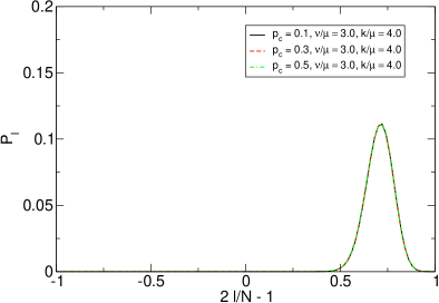
Figure 6: Probability distributions for two-parent recombination in the parallel model for the quadratic fitness $f(u)=ku^{2}/2$, with $k/\mu=4.0$ and $\nu/\mu=3.0$, obtained from stochastic simulations with $M=10~{}000$ sequences of $N=100$ bases and different values of $p_{c}$.

The system of differential equations (51) provides an exact representation of the evolution dynamics for an infinite population, when uniform crossover probability $p_{c}=1/2$ is assumed. On the other hand, our analytical equations Eq. (66), Eq. (67) for smooth fitness, or Eq. (72) for the discontinuous sharp peak, predict that the equilibrium results should be independent of the crossover probability $p_{c}$. To test this theory, we performed exact stochastic simulations based on a Lebowitz/Gillespie algorithm Bortz et al. (1995); Gillespie (1976). We generate a population of $M=10\,000$ sequences initially in the wild-type. The size of the finite population represented in the simulation was chosen large enough such that the results become independent of size $M$. Then, the population is evolved in time by point mutation, recombination and replication with rates proportional to $\mu$, $\nu$, and $f(u^{l})$ respectively, with $u^{l}=\frac{1}{N}\sum_{j=1}^{N}s_{j}^{l}$ the average composition of sequence $S_{l}$, $1\leq l\leq M$. For that purpose, a list is generated by defining: $\tau_{l}=\mu+\nu+f(u^{l})$, $\tau=\sum_{l=1}^{M}\tau_{l}$. With probability $\tau_{l}/\tau$, a sequence $1\leq l\leq M$ is chosen from the population to undergo either a single point mutation with probability $\mu/\tau_{l}$, replication with probability $f(u^{l})/\tau_{l}$, or recombination with another sequence with probability $\nu/\tau_{l}$ according to the process described in Fig. 4.

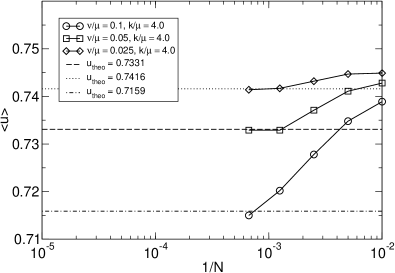
Figure 7: Convergence of the numerical results towards the theoretical value for two-parent recombination in the parallel model for the selective phase S1 in Eq. (75). In this example, $k/\mu=4.0$ and $\nu/\mu<1/8$.

To preserve the size $M$ of the population, when replication or recombination is performed, a sequence chosen at random from the population is substituted with the offspring. The time increment after any of these events is performed is calculated as $dt=-\log(w)/(N\tau)$, with $w\in(0,1]$ a uniformly distributed random number. The results obtained from this stochastic simulation are compared with the theoretical prediction in Table 7 for the sharp peak fitness landscape and uniform crossover $p_{c}=1/2$.

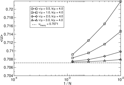
Figure 8: Convergence of the numerical results towards the theoretical value for two-parent recombination in the parallel model for the selective phase S2 in Eq. (75). In this example, $k/\mu=4.0$ and $\nu/\mu>1/8$.

In agreement with our theoretical prediction, as shown in Table 6 from stochastic simulations in the quadratic fitness landscape, the effect of recombination is independent of the polymerase crossover probability $p_{c}$. The probability distributions obtained for the systems considered in Table 6 are displayed in Fig. 6. Clearly, the distributions are independent of $p_{c}$, in agreement with the theory.

We obtain a direct numerical solution of the deterministic system of differential equations Eq. (51), which provides an exact representation of the evolution dynamics for an infinite population experiencing uniform crossover recombination $p_{c}=1/2$. A comparison between these numerical solutions, and results obtained from the stochastic simulation for a system large enough to eliminate finite size effects, is displayed in Table 7 for the sharp peak fitness. The theoretical prediction from the analytical formula Eq. (72) is also shown for comparison. It is evident from this table that the effect of recombination is independent of the polymerase crossover probability $p_{c}$, in agreement with our theoretical predictions.

Table 7: Stochastic process versus differential equation for two-parent recombination in the parallel model for the sharp peak fitness, $A/\mu$ = 4.0, N = 400.

$\nu/\mu$	$u^{\rm{stochastic}}$	$u^{\rm{diffeq}}$	$P_{0}^{\rm{stochastic}},\>p_{c}=0.1$	$P_{0}^{\rm{stochastic}},\>p_{c}=0.3$	$P_{0}^{\rm{stochastic}},\>p_{c}=0.5$	$P_{0}^{\rm{diffeq}}$	$P_{0}^{\rm{analytic}}$
0.0	0.998337	0.998336	0.75017	0.75017	0.75017	0.75016	0.75
1.0	0.998329	0.998326	0.7455	0.7454	0.74591	0.74544	0.7449
2.0	0.998312	0.998317	0.7415	0.7414	0.74085	0.74140	0.7398

From the data presented in Table 7, we notice that the deterministic system of differential equations provides an accurate representation of the underlying stochastic dynamics for the case of uniform crossover, $p_{c}=1/2$. Thus, the results obtained from the numerical solution of the deterministic system of differential equations can be fairly compared with the analytical theory.

It is remarkable that the small, but finite, effect introduced by recombination in the structure of the quasi-species distribution for the sharp peak case, is not a consequence of the Muller’s ratchet phenomenon Muller (1964) characteristic of finite populations. Indeed, the shift in the wild-type probability $P_{0}$ due to recombination, as predicted from our analytical equation Eq. (72), was derived from the system of differential equations Eq. (51), which describes the time evolution of an infinite population. Moreover, this closed analytical result is in excellent agreement with the numerical solution of the system of differential equations Eq. (51), as displayed in Fig. 8 and Table 8. A good agreement between our analytical and differential equation results, which correspond to the infinite population case, and the stochastic simulation is expected when the later is performed in a large enough population. We determined that for the parameters we consider, $M=10\,000$ sequences provides simulation results that are independent of the population size for the sharp peak fitness function, thus allowing for a comparison with the infinite population theory expressed by the differential equations Eq. (51) and with our analytical solution Eq. (72).

Table 8: Analytical theory versus numerical solution for two-parent recombination in the parallel model for the quadratic fitness $f(u)=ku^{2}/2$ with $N=800$ and $k/\mu$=4.0.

$\nu/\mu$	$u^{\rm{diffeq}}$	$u^{\rm{analytic}}$
0.0	0.7499	0.7500
0.025	0.7417	0.7416
0.05	0.7329	0.7331
0.1	0.7202	0.7159
0.5	0.7091	0.7071
1.0	0.7083	0.7071
2.0	0.7075	0.7071
3.0	0.7073	0.7071

Notice that for the quadratic fitness, the analytical theory reproduces the differential equation results within $\mathcal{O}(N^{-1})$. The convergence towards the theoretical value as a function of the system size $1/N$, for parameters within the $S1$ phase defined in Eq. (75), is displayed in Fig. 7, and for the S2 phase in Fig. 8.

As a final example, we apply our analytical solution Eq. (66) and Eq. (67) to study the square-root fitness, $f(u)=k\sqrt{|u|}$, as displayed in Table 9, where analytical theory and direct numerical solution of the differential equation agree to $\mathcal{O}(N^{-1})$.

Table 9: Analytical theory versus numerical solution for two-parent recombination in the parallel model for the square-root fitness $f(u)=k\sqrt{|u|}$, with $N=400,800,1000$ and $k/\mu$=4.0.

$\nu/\mu$	$u^{\rm{diffeq}},N=400$	$u^{\rm{diffeq}},N=800$	$u^{\rm{diffeq}},N=1000$	$u^{\rm{analytic}}$
0.0	0.6527	0.6525	0.65249	0.6523
0.1	0.6650	0.6672	0.6678	0.6710
0.3	0.6686	0.6697	0.66993	0.6710
0.5	0.6696	0.6703	0.67043	0.6710
0.8	0.6703	0.6707	0.67073	0.6710
1.0	0.6705	0.6708	0.67083	0.6710

As shown in Table 9, two-parent recombination in the square-root fitness landscape enhances selection towards sequences which are on average more fit, as observed by a slight increase of the average composition $u$, with respect to the case when recombination is absent. This effect, which was already observed for the square-root landscape in the presence of horizontal gene transfer, can be attributed to the negative (see Fig.1) epistatic interactions introduced by the square-root fitness, in agreement with the mutational deterministic hypothesis, Appendix N.

An additional interesting effect in two-parent recombination, which was observed in the quadratic as well as in the square-root fitness landscapes, is the presence of spectral rigidity: the effect of recombination becomes independent of the recombination rate for $\nu>0$.

In summary, from our generalization of the parallel or Crow-Kimura model for an infinite population of evolving sequences Eq. (38), we conclude that two-parent recombination introduces a mild mutational load over discontinuous fitness functions, such as a single sharp peak, and thus it can shift the error-threshold transition. For smooth fitness functions, the effect of recombination depends on the sign of epistasis (see Fig. 1), in agreement with the mutational deterministic hypothesis Kimura and Maruyama (1966); Kondrashov (1988, 1993, 1982). We show this analytically in Appendix N.

In contrast with horizontal gene transfer, recombination affects the structure of the quasi-species (and the error threshold transition) for a sharp peak fitness. We believe that this fundamental difference between horizontal gene transfer and recombination is because of the fact that the latter can generate a much larger diversity in the offspring per recombination event. Hence, the diversity barrier that, as previously discussed in section II, is imposed by the sharp exponential distribution in the sharp peak case can be tunneled through due to the more radical mixing effects of two-parent recombination. Our analytical theory, which provides explicit expressions for the mean fitness $f_{m}$ and average composition $u$, is developed in the realistic regime ($N\rightarrow\infty$), considering that typical viral genomes are $N\sim 10^{3}-10^{4}$.

III The Eigen model

In this section, we present a generalization of the classical Eigen model Eigen and Schuster (1971); Eigen et al. (1988, 1989), including the exchange of genetic material between pairs of individuals in an infinite population Park and Deem (2007),

$$\frac{dq_{i}}{dt}=\sum_{j,k=1}^{2^{N}}[B_{ij}C_{jk}r_{k}-\delta_{ij}\delta_{ik}D_{i}]q_{k}$$ (76)

Here, recombination as well as mutation are considered to be coupled to the replication process. Recombination is represented by the coefficients $C_{jk}$, which in general will be functions of the frequencies $q_{k}$, $C_{jk}\sim\delta_{jk}+\sum_{l}q_{l}\tilde{C}^{j}_{kl}/\sum_{k^{\prime}}q_{k^{\prime}}$.

III.1 Horizontal gene transfer of non-overlapping blocks

In this recombination scheme, we consider the exchange of blocks of genetic material between pairs of individuals in the population. We consider the blocks to be non-overlapping, such that we have $N/\bar{M}$ of them. We define a block index $0\leq b\leq N/\bar{M}-1$, and a site index within each block to be $\bar{M}b+1\leq j_{b}\leq\bar{M}(b+1)$. For this process, we have that the nonlinear recombination term in the differential Eq. (76) is

$$C_{jk} \sim \left(1-\frac{\nu/\bar{M}}{N/\bar{M}}\right)\delta_{j,k}+\frac{\nu/\bar{M}}{N/\bar{M}}$$ (77)

$$\times\prod_{b=0}^{N/\bar{M}-1}\left[\prod_{j_{b}=\bar{M}b+1}^{\bar{M}(b+1)}\delta_{s_{j_{b}}^{j},s_{j_{b}}^{k}}\left(\delta_{s_{j_{b}},+1}\frac{1+u(j_{b})}{2}+\delta_{s_{j_{b}},-1}\frac{1-u(j_{b})}{2}\right)\right]\prod_{m\neq\{j_{b}\}}\delta_{s_{m}^{j},s_{m}^{k}}$$

The recombination operator representing this process, assuming the recombination rate per block to be $\nu/\bar{M}$, becomes

$$\hat{R}=\prod_{b=0}^{N/\bar{M}-1}\left[\left(1-\frac{\nu/\bar{M}}{N/\bar{M}}\right)\prod_{j_{b}=\bar{M}b+1}^{\bar{M}(b+1)}\hat{I}_{j_{b}}+\frac{\nu/\bar{M}}{N/\bar{M}}\prod_{j_{b}=\bar{M}b+1}^{\bar{M}(b+1)}\hat{R}_{j_{b}}\right]$$ (78)

Here, we defined the single-site recombination operator as $\hat{R}_{j}=\vec{\hat{a}}^{\dagger}(j)D\vec{\hat{a}}(j)$, with the matrix $D$ defined in Eq. (8). We consider the large N limit, while keeping $N/\bar{M}\simeq\mathcal{O}(N)$. Then, the recombination operator defined in Eq. (78) becomes, to order $\mathcal{O}(N^{-1})$

$$\hat{R}=e^{-\frac{\nu}{\bar{M}}}e^{\frac{\nu}{N}\sum_{b=0}^{N/\bar{M}-1}\prod_{j_{b}=\bar{M}b+1}^{\bar{M}(b+1)}\vec{\hat{a}}^{\dagger}(j)D\vec{\hat{a}}(j)}$$ (79)

III.1.1 The Hamiltonian

The Hamiltonian operator for the Eigen model, including the horizontal gene transfer process described by the operator Eq. (78) is given by

$$-\hat{H} = Ne^{-\mu+\frac{\mu}{N}\sum_{j=1}^{N}\vec{\hat{a}}^{\dagger}(j)\sigma_{1}\vec{\hat{a}}(j)}e^{-\frac{\nu}{\bar{M}}+\frac{\nu}{N}\sum_{b=0}^{N/\bar{M}-1}\prod_{j_{b}=\bar{M}b+1}^{\bar{M}(b+1)}\left[\vec{\hat{a}}^{\dagger}(j_{b})D\vec{\hat{a}}(j_{b})\right]}$$ (80)

$$\times f\left[\frac{1}{N}\sum_{j=1}^{N}\vec{\hat{a}}^{\dagger}(j)\sigma_{3}\vec{\hat{a}}(j)\right]-Nd\left[\frac{1}{N}\sum_{j=1}^{N}\vec{\hat{a}}^{\dagger}(j)\sigma_{3}\vec{\hat{a}}(j)\right]$$

The microscopic fitness function is $f(u)$ and degradation function is $d(u)$. Here, the matrix $D$ is defined as in Eq. (8). We introduce a Trotter factorization of the evolution operator, in the basis of coherent states

$$e^{-\hat{H}t}=\lim_{M\rightarrow\infty}\int\left[\prod_{k=1}^{M}\mathcal{D}\vec{z}_{k}^{*}\mathcal{D}\vec{z}_{k}\right]|\vec{z}_{M}\rangle\left(\prod_{k=1}^{M}\langle\vec{z}_{k}|e^{-\epsilon\hat{H}}|\vec{z}_{k-1}\rangle\right)\langle\vec{z}_{0}|$$ (81)

As shown in Appendix H, the partition function is

$$Z=\int\left[\mathcal{D}\bar{\xi}\mathcal{D}\xi\mathcal{D}\bar{\eta}\mathcal{D}\eta\mathcal{D}\bar{\phi}\mathcal{D}\phi\right]e^{-S\left[\bar{\xi},\xi,\bar{\eta},\eta,\bar{\phi},\phi\right]}$$ (82)

Here, the action is defined by

$$S\left[\bar{\xi},\xi,\bar{\eta},\eta,\bar{\phi},\phi\right]=-N\int_{0}^{t}dt\left[-\bar{\xi}\xi-\bar{\eta}\eta-\bar{\phi}\phi+e^{-\mu(1-\eta)-\nu/\bar{M}+\frac{\nu}{\bar{M}}\phi^{\bar{M}}}f(\xi)-d(\xi)\right]-N\ln Q$$

(83)

III.1.2 The saddle point limit

We consider the saddle point limit of the action defined by Eq. (83). In the saddle point limit, for long times, the trace defined by Eq. (251) becomes

$$\lim_{t\rightarrow\infty}\frac{\ln Q_{c}}{t}=\frac{\bar{\phi}_{c}}{2}+\left[\bar{\xi}_{c}(\bar{\xi}_{c}+u\bar{\phi}_{c})+(\bar{\eta}_{c}+\bar{\phi}_{c}/2)^{2}\right]^{1/2}$$ (84)

In this saddle-point limit, the action is given by

$$\lim_{N,t\rightarrow\infty}\frac{\ln Z}{Nt} = \lim_{t\rightarrow\infty}\frac{-S_{c}}{Nt}$$

$$= \max_{\xi_{c},\bar{\xi}_{c},\phi_{c},\bar{\phi}_{c},\eta_{c},\bar{\eta}_{c}}\bigg{\{}f(\xi_{c})e^{-\mu(1-\eta_{c})-\frac{\nu}{\bar{M}}+\frac{\nu}{\bar{M}}\phi_{c}^{\bar{M}}}-d(\xi_{c})-\bar{\xi}_{c}\xi_{c}-\bar{\eta}_{c}\eta_{c}-\bar{\phi}_{c}\phi_{c}$$

$$+\frac{\bar{\phi}_{c}}{2}+\left[\bar{\xi}_{c}(\bar{\xi}_{c}+u\bar{\phi}_{c})+(\bar{\eta}_{c}+\bar{\phi}_{c}/2)^{2}\right]^{1/2}\bigg{\}}$$

As shown in Appendix I the mean fitness, defined from the saddle point action $f_{m}=\lim_{N,t\rightarrow\infty}\ln Z/Nt=-S_{c}/Nt$, is

$$f_{m}=\max_{-1\leq\xi_{c}\leq 1}\left\{e^{-\mu[1-\eta_{c}(\xi_{c})]-\frac{\nu}{\bar{M}}\{1-[\phi_{c}(\xi_{c})]^{\bar{M}}\}}f(\xi_{c})-d(\xi_{c})\right\}$$ (86)

Here, the expressions $\phi_{c}(\xi_{c})$ and $\eta_{c}(\xi_{c})$ are given by

$$\phi_{c}(\xi_{c})=\frac{1+u\xi_{c}}{2}+\frac{\sqrt{1-\xi_{c}^{2}}}{2}\frac{\mu+\frac{\nu}{2}(1-u^{2})\phi_{c}^{\bar{M}-1}}{\left[\left(\mu+\frac{\nu}{2}\phi_{c}^{\bar{M}-1}\right)^{2}-\frac{\nu^{2}u^{2}}{4}[\phi_{c}^{\bar{M}-1}]^{2}\right]^{1/2}}$$ (87)

$$\eta_{c}(\xi_{c})=\sqrt{1-\xi_{c}^{2}}\frac{\mu+\frac{\nu}{2}\phi_{c}^{\bar{M}-1}}{\left[\left(\mu+\frac{\nu}{2}\phi_{c}^{\bar{M}-1}\right)^{2}-\frac{\nu^{2}u^{2}}{4}[\phi_{c}^{\bar{M}-1}]^{2}\right]^{1/2}}$$ (88)

The average composition, $u$, is obtained from the self-consistency condition $f_{m}=f(u)-d(u)$.

Eq. (86) is an exact analytical expression for the equilibrium mean fitness of an infinite population of evolving sequences. This analytical expression is valid for arbitrary permutation invariant replication rate $f(u)$ and degradation rate $d(u)$.

III.1.3 Examples

We consider first the quadratic fitness case, $f(u)=ku^{2}/2+k_{0}$. By expanding the formulas Eqs. (86), (87) and (88) near the error threshold $\xi_{c}\sim 0$, $u\sim 0$, we obtain the phase boundary from the critical condition

$$k_{\rm{crit}}=\mu k_{0}\frac{1+\nu/\mu}{1+\nu/2\mu}$$ (89)

We notice that the phase boundary is qualitatively similar to the horizontal gene transfer process analyzed in section II. A 2, Eq. (14) for the parallel model. As in this former case, we notice that horizontal gene transfer introduces a mild mutational load against selection for a smooth fitness (i.e. quadratic).

As a second example, we consider the square-root fitness landscape $f(u)=k\sqrt{|u|}+1$. In Table 10, we evaluate our analytical Eqs. (86–88) for this particular case.

Table 10: Analytical results for horizontal gene transfer in the Eigen model for the square-root fitness $f(u)=k\sqrt{|u|}+1$, with $\bar{M}=3$.

$k$	$\nu$	$u^{\rm{analytic}}$
3.0	0.0	0.3346
3.0	0.5	0.3398
3.0	0.8	0.3422
3.0	1.5	0.3466
5.0	0.0	0.3588
5.0	0.5	0.3642
5.0	0.8	0.3667
5.0	1.5	0.3713
8.0	0.0	0.3741
8.0	0.5	0.3796
8.0	0.8	0.3822
8.0	1.5	0.3869

From the results displayed in Table 10, we notice that horizontal gene transfer increases the average composition $u$ and therefore the mean fitness of the population. This effect, which is attributed to the negative epistasis introduced by the square-root fitness (see Fig. 1), is in agreement with the previous examples studied in the case of the parallel model, and with the mutational deterministic hypothesis Arjan et al. (2007); Azevedo et al. (2006); Phillips et al. (2000); Kondrashov (1993), as we prove in Appendix M.

As a third example, we consider the sharp peak fitness $f(u)=(A-A_{0})\delta_{u,1}+A_{0}$. In this case, the maximum in Eq. (86) corresponds to $\xi_{c}=1$. From Eqs. (87) and (88), we have $\xi_{c}=(1+u)/2$, $\eta_{c}=0$, and hence after Eq. (86)

$$f_{m}=Ae^{-\mu-\frac{\nu}{\bar{M}}\left[1-\left(\frac{1+u}{2}\right)^{\bar{M}}\right]}$$ (90)

The error threshold is given, for $u=0$ in Eq. (90), by the condition $Ae^{-\mu-\frac{\nu}{\bar{M}}[1-1/2^{\bar{M}}]}>A_{0}$. However, we notice that $f_{m}(u=1)=Ae^{-\mu}>f_{m}(u=0)$. Hence, in the selected phase we have $u=1-\mathcal{O}(N^{-1})$. The fraction of the population located at the peak $P_{0}$ is obtained from the self-consistency condition $f_{m}=AP_{0}+A_{0}(1-P_{0})$

$$P_{0}=\frac{Ae^{-\mu}-A_{0}}{A-A_{0}}$$ (91)

After Eq. (91), we find the true error threshold at $A_{\rm{crit}}=A_{0}e^{\mu}$, while the condition $Ae^{-\mu-\frac{\nu}{\bar{M}}[1-2^{-\bar{M}}]}>A_{0}$ represents the limit of metastability for initial conditions with $u\sim 0$. We notice that this result is similar to the exact solution in the absence of horizontal gene transfer Park and Deem (2006). Hence, as previously discussed in section I.A. for the parallel model, we conclude that horizontal gene transfer does not affect the structure of the quasi-species for a discontinuous, single sharp peak fitness.

III.2 Horizontal gene transfer for multiple-size blocks

In analogy with the model treated in Section II.B, we consider the natural extension of horizontal gene transfer of blocks with multiple size, with average $\langle\bar{M}\rangle$ and $\langle\bar{M}\rangle/N=\mathcal{O}(N^{-1})$. Following a similar analysis as in the derivation of Eq. (27), we define the recombination operator for multiple-size blocks as

$$\hat{R}\sim e^{-\langle\bar{M}\rangle+\frac{\langle\bar{M}\rangle}{N}\sum_{j=1}^{N}\vec{\hat{a}}^{\dagger}(j)D\vec{\hat{a}}(j)}$$ (92)

III.2.1 The Hamiltonian

We consider horizontal gene transfer to be coupled to the replication process. Moreover, we will consider that when replication occurs, a horizontal gene transfer event also occurs with a probability $0\leq\nu/\langle\bar{M}\rangle\leq 1$. The Hamiltonian operator for the Eigen model, including the horizontal gene transfer process described by the operator Eq. (92) is given by

$$-\hat{H} = Ne^{-\mu+\frac{\mu}{N}\sum_{j=1}^{N}\vec{\hat{a}}^{\dagger}(j)D\vec{\hat{a}}(j)}\left(1-\frac{\nu}{\langle\bar{M}\rangle}+\frac{\nu}{\langle\bar{M}\rangle}e^{-\langle\bar{M}\rangle+\frac{\langle\bar{M}\rangle}{N}\sum_{j=1}^{N}\vec{\hat{a}}^{\dagger}(j)D\vec{\hat{a}}(j)}\right)$$

$$\times f\left[\frac{1}{N}\sum_{j=1}^{N}\vec{\hat{a}}^{\dagger}(j)\sigma_{3}\vec{\hat{a}}(j)\right]-Nd\left[\frac{1}{N}\sum_{j=1}^{N}\vec{\hat{a}}^{\dagger}(j)\sigma_{3}\vec{\hat{a}}(j)\right]$$

We introduce a Trotter factorization

$$e^{-\hat{H}t}=\lim_{M\rightarrow\infty}\int[\mathcal{D}\vec{z}^{*}\mathcal{D}\vec{z}]|\vec{z}_{M}\rangle\left(\prod_{j=1}^{M}\langle\vec{z}_{k}|e^{-\epsilon\hat{H}}|\vec{z}_{k-1}\right)\langle\vec{z}_{0}|$$ (94)

As shown in Appendix J, the partition function is

$$Z=\int\left[\mathcal{D}\bar{\xi}\mathcal{D}\xi\mathcal{D}\bar{\eta}\mathcal{D}\eta\mathcal{D}\bar{\phi}\mathcal{D}\phi\right]e^{-S\left[\bar{\xi},\xi,\bar{\eta},\eta,\bar{\phi},\phi\right]}$$ (95)

Here, the action in the continuous time limit is

$$S\left[\bar{\xi},\xi,\bar{\eta},\eta,\bar{\phi},\phi\right] = -N\int_{0}^{t}dt^{\prime}\bigg{\{}-\bar{\xi}\xi-\bar{\eta}\eta-\bar{\phi}\phi$$ (96)

$$+e^{-\mu(1-\eta)}[1-\frac{\nu}{\langle\bar{M}\rangle}+\frac{\nu}{\langle\bar{M}\rangle}e^{-\langle\bar{M}\rangle(1-\phi)}]f(\xi)-d(\xi)\bigg{\}}-N\ln Q$$

III.2.2 The saddle point limit

The saddle point limit is exact as $N\rightarrow\infty$ in Eq. (96). After a similar procedure as in Section 3.A.2, we find the saddle point equation for the mean fitness

$$f_{m}=\max_{-1\leq\xi_{c}\leq 1}\left\{e^{-\mu(1-\eta_{c})}[1-\frac{\nu}{\langle\bar{M}\rangle}+\frac{\nu}{\langle\bar{M}\rangle}e^{-\langle\bar{M}\rangle(1-\phi_{c})}]f(\xi_{c})-d(\xi_{c})\right\}$$ (97)

Here, the fields $\eta_{c}$ and $\phi_{c}$ are expressed as functions of $\xi_{c}$

$$\eta_{c}(\xi_{c})=\sqrt{1-\xi_{c}^{2}}\frac{\frac{\nu}{\langle\bar{M}\rangle}+\left[1-\frac{\nu}{\langle\bar{M}\rangle}\right]e^{\langle\bar{M}\rangle(1-\phi_{c})}+\frac{\nu}{2\mu}}{\left[\left(\frac{\nu}{\langle\bar{M}\rangle}+\left[1-\frac{\nu}{\langle\bar{M}\rangle}\right]e^{\langle\bar{M}\rangle(1-\phi_{c})}+\frac{\nu}{2\mu}\right)^{2}-\frac{u^{2}\nu^{2}}{4\mu^{2}}\right]^{1/2}}$$ (98)

$$\phi_{c}(\xi_{c})=\frac{1+u\xi_{c}}{2}+\frac{\sqrt{1-\xi_{c}^{2}}}{2}\frac{\frac{\nu}{\langle\bar{M}\rangle}+\left[1-\frac{\nu}{\langle\bar{M}\rangle}\right]e^{\langle\bar{M}\rangle(1-\phi_{c})}+\frac{\nu(1-u^{2})}{2\mu}}{\left[\left(\frac{\nu}{\langle\bar{M}\rangle}+\left[1-\frac{\nu}{\langle\bar{M}\rangle}\right]e^{\langle\bar{M}\rangle(1-\phi_{c})}+\frac{\nu}{2\mu}\right)^{2}-\frac{u^{2}\nu^{2}}{4\mu^{2}}\right]^{1/2}}$$ (99)

Equations (97)–(99) represent an exact analytical solution for the equilibrium mean fitness of an infinite population experiencing horizontal gene transfer of variable blocks size. This expression is valid for arbitrary, permutation invariant replication rate $f(u)$ and degradation rate $d(u)$.

III.2.3 Examples

We consider first the sharp peak fitness $f(u)=(A-A_{0})\delta_{u,1}+A_{0}$. In this case, the maximum in Eq. (97) is at $\xi_{c}=1$. From Eqs. (98) and (99), we obtain $\eta_{c}=0$ and $\phi_{c}=(1+u)/2$. Substituting these values in Eq. (97), we obtain for the mean fitness

$$f_{m}=e^{-\mu}\left[1-\frac{\nu}{\langle\bar{M}\rangle}+\frac{\nu}{\langle\bar{M}\rangle}e^{-\langle\bar{M}\rangle(1-u)/2}\right]A$$ (100)

The error threshold for $u=0$ is obtained from Eq. (100) by the condition $Ae^{-\mu}\left[1-\frac{\nu}{\langle\bar{M}\rangle}+\frac{\nu}{\langle\bar{M}\rangle}e^{-\langle\bar{M}\rangle/2}\right]>A_{0}$. However, we notice that $f_{m}(u=1)=Ae^{-\mu}>f_{m}(u=0)$. Therefore, in the selected phase the average composition $u=1-\mathcal{O}(N^{-1})$, and the effect of recombination becomes negligible for the sharp peak fitness. The fraction of the population located at the peak $P_{0}$ is obtained from the self-consistency condition $f_{m}=AP_{0}+A_{0}(1-P_{0})$

$$P_{0}=\frac{Ae^{-\mu}-A_{0}}{A-A_{0}}$$ (101)

From this expression, we find that the true error threshold for the sharp peak fitness is $A_{\rm{crit}}=e^{\mu}A_{0}$, with the condition $Ae^{-\mu}\left[1-\frac{\nu}{\langle\bar{M}\rangle}+\frac{\nu}{\langle\bar{M}\rangle}e^{-\langle\bar{M}\rangle/2}\right]>A_{0}$ representing the limit for metastability for initial conditions with $u\sim 0$.

As a second example, we consider the quadratic fitness $f(u)=ku^{2}/2+k_{0}$. An analytical expression for the phase boundary is obtained from Eqs. (97), (98) and (99) near the error threshold $\xi_{c}\sim 0$, $u\sim 0$. We find

$$k_{\rm{crit}}=\mu k_{0}\frac{1+\frac{\nu}{\mu}}{1+\frac{\nu}{2\mu}}$$ (102)

For small $\nu$, the critical value is $k_{\rm{crit}}\sim k_{0}(\mu+\nu/2)$.

As a final example, we consider the square-root fitness $f(u)=k\sqrt{|u|}+1$. Analytical results, as obtained from Eqs. (97)–(99) for this case, are presented in Table 11.

Table 11: Analytical results for horizontal gene transfer in the Eigen model for the square-root fitness $f(u)=k\sqrt{|u|}+1$, with $\langle\bar{M}\rangle=3$.

$k$	$\nu$	$u^{\rm{analytic}}$
3.0	0.0	0.3346
3.0	0.5	0.3409
3.0	0.8	0.3450
3.0	1.5	0.3546
5.0	0.0	0.3588
5.0	0.5	0.3654
5.0	0.8	0.3695
5.0	1.5	0.3794
8.0	0.0	0.3741
8.0	0.5	0.3809
8.0	0.8	0.3851
8.0	1.5	0.3950

We notice that the results obtained for the horizontal gene transfer process with variable block size agree with the corresponding ones when the size of the recombination blocks is fixed. We recall that this correspondence was also observed and discussed in the previous section for the parallel model, so similar arguments apply to the Eigen model as well. An analytical proof is provided in Appendix M.

III.3 The Eigen model with two-parent recombination

For the Eigen model, we introduce the recombination process described in Section II.C and illustrated in Fig. 4, which considers the exchange of genetic material between pairs of sequences due to crossovers governed by the polymerase switching from one parental chromosome to the other with probability $p_{c}$ per site. For the Eigen model, mutation and recombination are considered to be coupled to the recombination process, as stated in the generic differential equation Eq. (76). We will consider that during replication, a sequence can recombine with probability $\nu\leq 1$, or just replicate without recombining with probability $1-\nu$. This process is represented by the coefficients in Eq. (76)

$$C_{jk} = (1-\nu)\delta_{j,k}+\frac{\nu}{2}\sum_{\{\alpha_{n}=\pm 1\}}\left\{\left[\prod_{n=2}^{N}p_{c}^{\frac{1-\alpha_{n-1}\alpha_{n}}{2}}(1-p_{c})^{\frac{1+\alpha_{n-1}\alpha_{n}}{2}}\right]\right.$$

$$\times\left.\sum_{l=1}^{2^{N}}p_{l}\prod_{n=1}^{N}\left(\frac{1+s_{n}^{k}s_{n}^{j}}{2}\right)^{\frac{1+\alpha_{n}}{2}}\left(\frac{1+s_{n}^{l}}{2}\delta_{s_{n}^{j},+1}+\frac{1-s_{n}^{l}}{2}\delta_{s_{n}^{j},-1}\right)^{\frac{1-\alpha_{n}}{2}}\right\}$$

Here, again, $p_{l}=q_{l}/\sum_{l=1}^{2^{N}}q_{l}$ is the normalized probability for the sequence $1\leq l\leq 2^{N}$.

In the spin Boson representation, we express the Eigen model Hamiltonian by the operator

$$-\hat{H} = Ne^{-\mu+\frac{\mu}{N}\sum_{j=1}^{N}\vec{\hat{a}}^{\dagger}(j)\sigma_{1}\vec{\hat{a}}(j)}\left[(1-\nu)\hat{I}+\nu g[\{\vec{\hat{a}}^{\dagger}(j)D_{j}^{l}\vec{\hat{a}}(j)\}]\right]$$ (104)

$$\times f\left[\frac{1}{N}\sum_{j=1}^{N}\vec{\hat{a}}^{\dagger}(j)\sigma_{3}\vec{\hat{a}}(j)\right]-Nd\left[\frac{1}{N}\sum_{j=1}^{N}\vec{\hat{a}}^{\dagger}(j)\sigma_{3}\vec{\hat{a}}(j)\right]$$

Here, $g[\{\hat{R}_{j}^{l}\}]$ was defined in Eq. (39), and the matrices $D_{j}^{l}$ were defined in Eq. (42). We introduce a Trotter factorization

$$e^{-\hat{H}t}=\lim_{M\rightarrow\infty}\int[\mathcal{D}\vec{z}^{*}\mathcal{D}\vec{z}]|\vec{z}_{M}\rangle\left(\prod_{k=1}^{M}\langle\vec{z}_{k}|e^{-\epsilon\hat{H}}|\vec{z}_{k-1}\rangle\right)\langle\vec{z}_{0}|$$ (105)

As shown in Appendix K, the partition function is

$$Z=\int\mathcal{D}\bar{\xi}\mathcal{D}\xi\mathcal{D}\bar{\eta}\mathcal{D}\eta\mathcal{D}\bar{\phi}\mathcal{D}\phi e^{-S[\bar{\xi},\xi,\bar{\eta},\eta,\bar{\phi},\phi]}$$ (106)

Here, the action is defined by

$$S[\bar{\xi},\xi,\bar{\eta},\eta,\bar{\phi},\phi] = -N\int_{0}^{t}dt^{\prime}\left[-\bar{\xi}\xi-\bar{\eta}\eta-\bar{\phi}\phi\right.$$

$$+\left.e^{-\mu(1-\eta)}(1-\nu+\nu g(\phi))f(\xi)-d(\xi)\right]-N\ln Q$$

III.3.1 The saddle point limit

For long times, a steady state condition is achieved. Then, the fields become time-independent, and we have

$$\lim_{t\rightarrow\infty}\frac{\ln Q_{c}}{t}=\frac{\bar{\phi}_{c}}{2}+\left[\bar{\xi}_{c}(\bar{\xi}_{c}+u\bar{\phi}_{c})+\left(\bar{\eta}_{c}+\frac{\bar{\phi}_{c}}{2}\right)^{2}\right]^{1/2}$$ (108)

We look for the saddle point solution from the action

$$\lim_{N,t\rightarrow\infty}\frac{\ln Z}{Nt}=\lim_{t\rightarrow\infty}\frac{-S_{c}}{Nt} = \max_{\bar{\xi}_{c},\xi_{c},\bar{\eta}_{c},\eta_{c},\bar{\phi}_{c},\phi_{c}}\bigg{\{}-\bar{\xi}_{c}\xi_{c}-\bar{\eta}_{c}\eta_{c}-\bar{\phi}_{c}\phi_{c}+e^{-\mu(1-\eta_{c})}(1-\nu+\nu g(\phi_{c}))f(\xi_{c})$$ (109)

$$-d(\xi_{c})+\frac{\bar{\phi}_{c}}{2}+\left[\bar{\xi}_{c}(\bar{\xi}_{c}+u\bar{\phi}_{c})+\left(\bar{\eta}_{c}+\frac{\bar{\phi}_{c}}{2}\right)^{2}\right]^{1/2}\bigg{\}}$$

Because of the singular behavior of the function $g(\phi_{c})$, to find the saddle point we need to consider three separate cases: $\phi_{c}<1$, $\phi_{c}=1$, and $\phi_{c}=1-\mathcal{O}(1/N)$. We notice that the saddle point analysis may not apply exactly, unless $g(\phi_{c})=\delta_{\phi_{c},1}$.

Case 1: $\phi_{c}<1$. The mean fitness is given by

$$f_{m}^{(1)}=\max_{-1\leq\xi_{c}\leq 1}\{(1-\nu)e^{-\mu\left[1-\sqrt{1-\xi_{c}^{2}}\right]}f(\xi_{c})-d(\xi_{c})\}$$ (110)

We note $\phi_{c}$ is still given by Eq. (65).

Case 2: $\phi_{c}=1$. The mean fitness is given by

$$f_{m}^{(2)}=\max_{-1\leq\xi_{c}\leq 1}\{e^{-\mu\left[1-\frac{1-u\xi_{c}-|u\xi_{c}-u^{2}|}{1-u^{2}}\right]}f(\xi_{c})-d(\xi_{c})\}$$ (111)

Case 3: $\phi_{c}=1-\mathcal{O}(1/N)$. In this case, additional analysis is necessary to calculate the mean fitness due to the singular behavior of the $g(\phi_{c})$ function. For a smooth fitness function, we can argue this case does not exist. We first consider the Hamiltonian (104) for the case $g=0$. In this case, the fitness function is simply multiplied by $(1-\nu)$. If the degradation function is zero, the largest eigenvalue, $f_{m}$ is simply multiplied by $(1-\nu)$ relative to the $\nu=0$ case. Without degradation, this result allows us to calculate the average composition, $u_{*}$, from the implicit relation $f_{m}(\nu)=(1-\nu)f_{m}(\nu=0)=f(u_{*})$. With a non-zero degradation function, the equation for $f_{m}(\nu)$ will be a bit more involved. Alternatively, if we consider the differential equation for the unnormalized class probabilities, $dQ/dt=LQ$, we see that the differential operator $L$ looks like that in the absence of recombination, save for a multiplication of $(1-\nu)$ in the fitness function. Thus, the variance of the population is given by Park and Deem (2006) $\sigma^{2}_{u}/N=2\mu u_{*}(1-\nu)f(u_{*})/[N((1-\nu)f^{\prime}(u_{*})-d^{\prime}(u_{*}))]$. Considering more carefully the $g$ function, we find as before this term is exponentially negligible compared to the $-\nu P(u)$ term when $\sigma^{2}<\sigma_{u}^{2}$. In other words, we must strictly be in case 1 when

$$1-u_{*}^{2}<2\mu u_{*}(1-\nu)f(u_{*})/[(1-\nu)f^{\prime}(u_{*})-d^{\prime}(u_{*})]$$ (112)

We denote the value of $\nu$ at which

$$1-u_{*}^{2}=2\mu u_{*}(1-\nu)f(u_{*})/[(1-\nu)f^{\prime}(u_{*})-d^{\prime}(u_{*})]{\rm~{}at~{}}\nu=\nu_{*}$$ (113)

as $\nu_{*}$. Now, at this value of $\nu_{*}$ we have $\int d{u_{1}}d{u_{2}}R_{u_{1}u_{2}}^{u}P(u_{1})P(u_{2})=P(u)$. Thus, the term proportional to $\nu$ in Hamiltonian (104) exactly vanishes. Thus, we have $df_{m}/d\nu=0$ and $dP(u)/d\nu=0$ at this value of $\nu$. There is spectral rigidity. This result implies that for $\nu>\nu_{*}$, the distribution $P(u)$ is independent of $\nu$, and that the value of $u_{*}$ is constant. In other words, the value of $f_{m}$ in case 2 must be constant with $\nu$. Assuming $f_{m}$ varies continuously with $\nu$ in case 1, and that the fitness values for case 1 and case 2 are equal at a single value of $\nu$, which mathematically may be negative, case 2 is simply case 1 with the value $\nu=\nu_{*}$

$$f_{m}(\nu>\nu_{*})=f_{m}(\nu=\nu_{*})$$ (114)

Equations (110), (111) constitute an exact analytical expression for the equilibrium mean fitness of an infinite population of sequences evolving under the dynamics of the Eigen model, and experiencing two-parent recombination. These equations are exact for a smooth, permutation invariant replication rate $f(u)$ and degradation rate $d(u)$.

For a non-smooth fitness function, additional analysis is necessary, since $f^{\prime}(u_{*})-d^{\prime}(u_{*})$ is undefined, and $P(u)$ may no longer be Gaussian.

III.3.2 Examples

We investigate the phase diagrams, as predicted from our theoretical equations, for two different fitness functions: A sharp peak and a quadratic fitness landscape.

As an example, we consider the sharp peak fitness, $f(u)=(A-A_{0})\delta_{u,1}+A_{0}$. The maximum is obtained at $\xi_{c}=1$, $u=1-\mathcal{O}(N^{-1})$. From Eqs. (111) and (110) we have

$$f_{m}^{(2)}=Ae^{-\mu}>f_{m}^{(1)}=(1-\nu)Ae^{-\mu}$$ (115)

Hence, for the sharp peak fitness a single selective phase is observed. In this case, the function $g(\phi_{c})$ is not exactly a Kronecker delta $\delta_{\phi_{c},1}$, we are in case 3, and then we expect to observe a small correction, approximately linear in $\nu$ from the prediction of the saddle point analysis. By considering the differential equations for the sharp peak case at zeroth-order in $\nu$, we find that the class distributions satisfy $e^{-\mu/2}\sum_{k}(r_{k}/N)P^{(0)}_{k}/2^{k}=f_{m}^{(0)}\sum_{l}P^{(0)}_{l}/2^{l}$ with $P^{(0)}_{0}=(Ae^{-\mu}-A_{0})/(A-A_{0})$ and $f^{(0)}_{m}=AP^{(0)}_{0}+A_{0}(1-P^{(0)}_{0})=Ae^{-\mu}$. Thus we find $S=\sum_{l}P^{(0)}_{l}/2^{l}=(A-A_{0})P^{(0)}_{0}e^{-\mu/2}/(f^{(0)}_{m}-A_{0}e^{-\mu/2})=(Ae^{-\mu}-A_{0})e^{-\mu/2}/(Ae^{-\mu}-A_{0}e^{-\mu/2})$. Thus, we find the recombination term $\sum_{k}(r_{k}/N)P^{(0)}_{k}/2^{k}\sum_{l}P^{(0)}_{l}/2^{l}=Ae^{-\mu/2}S^{2}$. Hence, we find that at first order in $\nu$, the fraction of the population located at the peak is given by

$$P_{0}=\frac{Ae^{-\mu}-A_{0}}{A-A_{0}}-\nu e^{-\mu}\left[\frac{A}{A-A_{0}}-Ae^{-\mu/2}\frac{Ae^{-\mu}-A_{0}}{(Ae^{-\mu/2}-A_{0})^{2}}\right]+\mathcal{O}(\nu^{2})$$ (116)

We note that this value of $f_{m}=AP_{0}+A_{0}(1-P_{0})$ interpolates between $f_{m}^{(1)}$ for $Ae^{-\mu}/A_{0}=1$ and a value intermediate to $f_{m}^{(1)}$ and $f_{m}^{(2)}$ for $Ae^{-\mu}/A_{0}=\infty$.

As a second example, we consider the quadratic fitness $f(u)=ku^{2}/2+k_{0}$. By maximizing expressions Eq. (111) not (c) and Eq. (110), we obtain two selective phases S1 and S2, and a non-selective phase NS, defined by the equations

$$S1:\;u = \left[2(1-\nu)e^{-\mu\left[1-\sqrt{1-\xi_{c}^{2}}\right]}(\xi_{c}^{2}/2+k_{0}/k)-2k_{0}/k\right]^{1/2},\quad\nu<\min(\nu_{*},\nu_{c})$$

$$S2:\;u = \left[\frac{1-2\mu k_{0}/k}{1+\mu}\right]^{1/2},\quad\nu_{c}>\nu_{*}<\nu$$

$$NS:\;u = 0,\quad{\rm otherwise}$$ (117)

where in the S1 phase

$$\xi_{c}^{2}=2[\sqrt{1+\mu^{2}(1+2k_{0}/k)}-1-\mu^{2}k_{0}/k]/\mu^{2}$$ (118)

and we have defined

$$\nu_{c} = 1-\frac{k_{0}}{k}e^{\mu\left[1-\sqrt{1-\xi_{c}^{2}}\right]}/(\xi_{c}^{2}/2+k_{0}/k)$$

$$\nu_{*} = 1-\frac{k+2k_{0}}{2k(1+\mu)}e^{\mu\left[1-\sqrt{1-\xi_{c}^{2}}\right]}/(\xi_{c}^{2}/2+k_{0}/k)$$ (119)

where $\xi_{c}^{2}$ is given by Eq. (118). The phase structure is defined by the conditions: For $2\mu k_{0}/k\geq 1$, the system is in S1 if $\nu<\nu_{c}$, or in NS if $\nu\geq\nu_{c}$; for $2\mu k_{0}/k<1$, the system is in S1 if $\nu\leq\nu_{*}$, or in S2 if $\nu>\nu_{*}$. From Eq. (119), we notice that at $2\mu k_{0}/k=1$, $\nu_{c}=\nu_{*}$.

We note that the phase transition between case 1 and case 2 is exactly as predicted by Eq. (113). We further note that the mean fitness is independent of $\nu$ for $\nu>\nu_{*}$, exactly as predicted by Eq. (114).

As a final example, we consider the square-root fitness $f(u)=k\sqrt{|u|}+1$. By maximizing expressions Eq. (111) not (c) and Eq. (110) for the square-root fitness landscape, we obtain the results presented in Table 12

Table 12: Analytical results for two-parent recombination in the Eigen model for the square-root fitness $f(u)=k\sqrt{|u|}+1$.

$k/\mu$	$\nu/\mu$	$u^{\rm{analytic}}$
4.0	0.0	0.3493
4.0	0.1	0.3892
4.0	0.2	0.3892
4.0	0.5	0.3892
3.0	0.0	0.3346
3.0	0.1	0.3892
3.0	0.2	0.3892
3.0	0.5	0.3892

From the results displayed in Table 12, we observe a similar qualitative behavior as in the two-parent recombination for the parallel case, Table 9. In the square-root fitness, recombination introduces a favorable effect over selection, which can be attributed to negative epistasis (see Fig. 1) according to the mutational deterministic hypothesis Arjan et al. (2007); Azevedo et al. (2006); Phillips et al. (2000); Kondrashov (1993), as shown in Appendix O. Spectral rigidity is also observed in this case when $\nu>0$.

IV Conclusion

We have generalized two classical models of evolutionary biology, the Crow-Kimura and Eigen models. We have introduced inter-individual transfer of genetic information to these models, bringing them closer to the modern understanding of evolutionary biology. For both models, we showed how to incorporate horizontal gene transfer. We showed that these generalized models may be written in an equivalent field-theoretic formulation. This mapping allows us to apply the powerful mathematical techniques of quantum field theory to obtain exact analytical solutions. For fitness landscapes that depend only on distance from a wild-type genome and for long genome lengths, we are able to solve for the mean population fitness for arbitrary functional forms of the fitness. Horizontal gene transfer of $\bar{M}$ genetic units was shown to be analogous to horizontal gene transfer of one genetic unit, with a suitably scaled horizontal gene transfer rate.

We also showed how to incorporate recombination to these classical models, as might occur in viral super- or co-infection. This case seems at first glance far more non-linear, since on average half of the genetic material is taken from each parent to make the child, rather than $O(1)$ genes as in horizontal gene transfer. Somewhat surprisingly, we were able to exactly solve the two-parent recombination case for both the Eigen and Crow-Kimura model as well. In the limit of a long genome and for fitness landscapes that depend on the distance from a wild-type genome, we find that the mean population fitness is independent of the average cross-over length in the recombination process. We also find two selected phases. The phase for large recombination rates is spectrally rigid, with the mean fitness and population distribution independent of the rate of recombination.

We proved the mutational deterministic hypothesis holds for horizontal gene transfer or recombination in both the parallel (Kimura) and Eigen models. That is, horizontal gene transfer and recombination reduce the mean fitness in the presence of positive epistasis and increase the fitness in the presence of negative epistasis (see Fig. 1 and Appendices L, M, N, and O).

For a discontinuous, sharp peak fitness landscape, we found that horizontal gene transfer does not affect the structure of the quasi-species distribution or the error threshold transition. For the sharp peak fitness function, the only appreciable effect of horizontal gene transfer is related to the potential emergence of metastability depending on the initial conditions, and we analytically determined the region of parameters space in which this situation may occur. On the other hand, even for the sharp peak fitness function, two-parent recombination induces enough mixing to enhance diversity in systems evolving under a sharp peak replication rate, thus changing the quasi-species distribution and shifting the error threshold transition. We found explicit analytical expressions for this shift.

For smooth fitness landscapes, these genetic transfers affect the steady-state population distribution and mean fitness. Recombination and horizontal gene transfer may, of course, dramatically change the dynamics of the evolution process as well. The most dramatic impact of these exchanges of genetic material is expected for fitness landscapes that have a correlated, biological structure that is conjugate to these exchanges Sun and Deem (2007). Analytic investigation of such correlated fitness landscapes is perhaps one of the next steps in the development of modern theories of evolution.

Appendix A

We consider Eq. (11) for horizontal gene transfer of blocks of fixed length $\bar{M}$ in the parallel model. For $\epsilon=t/M$ and $M\rightarrow\infty$, we have

$$\langle\vec{z}_{k}|e^{-\epsilon\hat{H}}|\vec{z}_{k-1}\rangle\simeq\langle\vec{z}_{k}|\vec{z}_{k-1}\rangle-\epsilon\langle\vec{z}_{k}|\hat{H}|\vec{z}_{k-1}\rangle\simeq\langle\vec{z}_{k}|\vec{z}_{k-1}\rangle e^{-\epsilon\frac{\langle\vec{z}_{k}|\hat{H}|\vec{z}_{k-1}\rangle}{\langle\vec{z}_{k}|\vec{z}_{k-1}\rangle}}.$$ (120)

For the Hamiltonian matrix elements in the coherent states basis, we obtain to order $\mathcal{O}(N^{0})$

$$-\frac{\langle\vec{z}_{k}|\hat{H}|\vec{z}_{k-1}\rangle}{\langle\vec{z}_{k}|\vec{z}_{k-1}\rangle} = Nf\left[\frac{1}{N}\sum_{j=1}^{N}\vec{z}^{*}_{k}(j)\sigma_{3}\vec{z}_{k-1}(j)\right]+\mu\sum_{j=1}^{N}[\vec{z}_{k}^{*}(j)\sigma_{1}\vec{z}_{k-1}(j)-1]$$ (121)

$$+\nu\sum_{b=0}^{N/\bar{M}-1}\left[\prod_{j_{b}=\bar{M}b+1}^{\bar{M}(b+1)}\vec{z}^{*}_{k}(j_{b})D\vec{z}_{k-1}(j_{b})-1\right]$$

We introduce the auxiliary field

$$\xi_{k}=\frac{1}{N}\sum_{j=1}^{N}\vec{z}_{k}^{*}(j)\sigma_{3}\vec{z}_{k-1}(j)$$ (122)

and the conjugate field $\bar{\xi}_{k}$ to enforce the constraint via a Laplace representations of the delta function. Substituting into Eq. (121) into Eq. (11), we obtain

$$e^{-\hat{H}t} = \lim_{M\rightarrow\infty}\int\left[\mathcal{D}\vec{z}^{*}\mathcal{D}\vec{z}\right]\int\left[\prod_{k=0}^{M}\frac{i\epsilon Nd\bar{\xi}_{k}d\xi_{k}}{2\pi}\right]|\vec{z}_{M}\rangle\langle\vec{z}_{0}|$$

$$\times e^{\sum_{k=1}^{M}\sum_{j=1}^{N}\left\{-1/2[\vec{z}_{k}^{*}(j)\cdot\vec{z}_{k}(j)+\vec{z}_{k-1}^{*}(j)\cdot\vec{z}_{k-1}(j)-2\vec{z}_{k}^{*}(j)\cdot\vec{z}_{k-1}(j)]+\epsilon[\vec{z}_{k}^{*}(j)(\bar{\xi}_{k}\sigma_{3}+\mu\sigma_{1})\vec{z}_{k-1}(j)]\right\}}$$

$$\times e^{-\epsilon N\sum_{k=1}^{M}\left[\bar{\xi}_{k}\xi_{k}+\mu+\frac{\nu}{\bar{M}}-f(\xi_{k})-\frac{\nu}{N}\sum_{b=0}^{N/\bar{M}-1}\prod_{j_{b}=\bar{M}b+1}^{\bar{M}(b+1)}\vec{z}_{k}^{*}(j_{b})D\vec{z}_{k-1}(j_{b})\right]}.$$

The contribution of the interaction term $\frac{\nu}{N}\sum_{b=0}^{N/\bar{M}-1}\prod_{j_{b}=\bar{M}b+1}^{\bar{M}(b+1)}\vec{z}_{k}^{*}(j_{b})D\vec{z}_{k-1}(j_{b})$ to the partition function can be treated to arbitrary order in perturbation theory using the formula $Z=Z_{0}\langle e^{-\delta S}\rangle_{0}$, and its contribution shown to be site-independent. Moreover, this reference perturbation theory has $\mathcal{O}(N^{-1})$ fluctuations. Thus, it can be shown that with an error $\mathcal{O}(\bar{M}/N)$ at all orders in perturbation theory, we obtain the same partition function when substituting this interaction term by $\frac{\nu}{\bar{M}}\left(1/N\sum_{j=1}^{N}\vec{z}_{k}^{*}(j)D\vec{z}_{k-1}(j)\right)^{\bar{M}}$. Therefore, we define the auxiliary field

$$\phi_{k}=\frac{1}{N}\sum_{j=1}^{N}\vec{z}_{k}^{*}(j)D\vec{z}_{k-1}(j).$$ (124)

We obtain the partition function from the trace of the evolution operator, Eq. (LABEL:eq13), projected onto physical states Park and Deem (2006)

$$Z={\rm{Tr}}\left[e^{-\hat{H}t}\hat{P}\right]=\int_{0}^{2\pi}\left[\prod_{j=1}^{N}\frac{d\lambda_{j}}{2\pi}e^{-i\lambda_{j}}\right]\lim_{M\rightarrow\infty}\int\left[\prod_{k=0}^{M}\mathcal{D}\vec{z}^{*}_{k}\mathcal{D}\vec{z}_{k}\right]\left.e^{-S[\vec{z}^{*},\vec{z}]}\right|_{\vec{z}_{0}=e^{i\lambda}\vec{z}_{M}}.$$ (125)

By inserting Eq. (124), we obtain

$$Z = \lim_{M\rightarrow\infty}\int\left[\mathcal{D}\bar{\xi}\mathcal{D}\xi\mathcal{D}\bar{\phi}\mathcal{D}\phi\right]e^{-N\epsilon\sum_{k=1}^{M}[\bar{\xi}_{k}\xi_{k}+\bar{\phi}_{k}\phi_{k}-f(\xi_{k})+\mu+\frac{\nu}{\bar{M}}-\frac{\nu}{\bar{M}}\phi_{k}^{\bar{M}}]}$$

$$\times\int_{0}^{2\pi}\left[\prod_{j=1}^{N}\frac{d\lambda_{j}}{2\pi}e^{-i\lambda_{j}}\right]\int\left[\prod_{k=0}^{M}\mathcal{D}\vec{z}_{k}^{*}\mathcal{D}\vec{z}_{k}\right]\left.e^{-\sum_{j=1}^{N}\sum_{k,l=1}^{M}\vec{z}_{k}^{*}(j)S_{kl}(j)\vec{z}_{l}(j)}\right|_{\vec{z}_{M}=e^{i\lambda}\vec{z}_{0}}$$

The matrix $S(j)$ in Eq. (LABEL:eq16) is defined by

$$S(j)=\left(\begin{array}[]{ccccc}I&0&0&\ldots&-e^{i\lambda_{j}}A_{1}\\ -A_{2}&I&0&\ldots&0\\ 0&-A_{3}&I&\ldots&0\\ \vdots&\ldots&\ldots&\ldots&0\\ 0&\ldots&0&-A_{M}&I\end{array}\right)$$ (132)

Here $A_{k}=I+\epsilon(\bar{\xi}_{k}\sigma_{3}+\mu\sigma_{1}+\bar{\phi}_{k}D)$.

After calculating the Gaussian integral over the coherent state fields, we obtain

$$\lim_{M\rightarrow\infty}\int_{0}^{2\pi}\prod_{j=1}^{N}\frac{d\lambda_{j}}{2\pi}e^{-i\lambda_{j}}\int\left[\prod_{k=0}^{M}\mathcal{D}\vec{z}^{*}_{k}\mathcal{D}\vec{z}_{k}\right]e^{-\sum_{j=1}^{N}\sum_{k,l=1}^{M}\vec{z}^{*}_{k}(j)S_{kl}(j)\vec{z}_{l}(j)}$$ (133)

$$= \lim_{M\rightarrow\infty}\int_{0}^{2\pi}\prod_{j=1}^{N}\frac{d\lambda_{j}}{2\pi}e^{-i\lambda_{j}}\left[\det S(j)\right]^{-1}$$

$$= \lim_{M\rightarrow\infty}\int_{0}^{2\pi}\prod_{j=1}^{N}\frac{d\lambda_{j}}{2\pi}e^{-i\lambda_{j}}e^{-{\rm{Tr}}\ln[I-e^{i\lambda_{j}}\hat{T}\exp(\epsilon\sum_{k=1}^{M}\bar{\xi}_{k}\sigma_{3}+\mu\sigma_{1}+\bar{\phi}_{k}D)]}$$

$$= \lim_{M\rightarrow\infty}\prod_{j=1}^{N}{\rm{Tr}}\>\hat{T}e^{\epsilon\sum_{k=1}^{M}(\bar{\xi}_{k}\sigma_{3}+\mu\sigma_{1}+\bar{\phi}_{k}D)}=Q^{N},$$

where $\hat{T}$ is the time ordering operator and

$$Q={\rm{Tr}}\>\hat{T}e^{\int_{0}^{t}dt^{\prime}(\bar{\xi}\sigma_{3}+\mu\sigma_{1}+\bar{\phi}D)}.$$ (134)

With this result the partition function in Eq. (LABEL:eq16) becomes Eq. (12).

Appendix B

From Eq. (15), we obtain the saddle-point equations with respect to the fields $\bar{\xi}_{c}$, $\bar{\phi}_{c}$ for horizontal gene transfer of blocks of fixed length $\bar{M}$ in the parallel model:

$$\frac{\delta}{\delta\bar{\xi}_{c}}\left(\frac{-S_{c}}{Nt}\right)=-\xi_{c}+\frac{2\bar{\xi}_{c}+u\bar{\phi}_{c}}{2\left[\bar{\xi}_{c}(\bar{\xi}_{c}+u\bar{\phi}_{c})+\left(\mu+\frac{\bar{\phi}_{c}}{2}\right)^{2}\right]^{1/2}}=0$$ (135)

$$\frac{\delta}{\delta\bar{\phi}_{c}}\left(\frac{-S_{c}}{Nt}\right)=-\phi_{c}+\frac{1}{2}+\frac{u\bar{\xi}_{c}+\mu+\frac{\bar{\phi}_{c}}{2}}{2\left[\bar{\xi}_{c}(\bar{\xi}_{c}+u\bar{\phi}_{c})+\left(\mu+\frac{\bar{\phi}_{c}}{2}\right)^{2}\right]^{1/2}}=0.$$ (136)

Then, the system of Eqs. (135) and (136) reduces to

$$\xi_{c}=\frac{\bar{\xi}_{c}+\frac{u}{2}\bar{\phi}_{c}}{\left[\bar{\xi}_{c}(\bar{\xi}_{c}+u\bar{\phi}_{c})+\left(\mu+\frac{\bar{\phi}_{c}}{2}\right)^{2}\right]^{1/2}}$$ (137)

$$\phi_{c}-\frac{1}{2}=\frac{u\bar{\xi}_{c}+\mu+\frac{\bar{\phi}_{c}}{2}}{2\left[\bar{\xi}_{c}(\bar{\xi}_{c}+u\bar{\phi}_{c})+\left(\mu+\frac{\bar{\phi}_{c}}{2}\right)^{2}\right]^{1/2}}.$$ (138)

We eliminate $\bar{\xi}_{c}$, $\bar{\phi}_{c}$, to obtain

$$\frac{-S_{c}}{Nt} = \max_{\xi_{c},\phi_{c}}\left\{f(\xi_{c})-\mu-\frac{\nu}{\bar{M}}+\frac{\nu}{\bar{M}}\phi_{c}^{\bar{M}}+\frac{\mu}{1-u^{2}}(2\phi_{c}-1-u\xi_{c})\right.$$ (139)

$$-\left.\frac{\mu|u|}{1-u^{2}}\left[(2\phi_{c}-1-u\xi_{c})^{2}-(1-u^{2})(1-\xi_{c}^{2})\right]^{1/2}\right\}.$$

Finally, we look for an extremum in $\phi_{c}$,

$$\frac{\delta}{\delta\phi_{c}}\left(\frac{-S_{c}}{Nt}\right)=\frac{\nu}{\bar{M}}\bar{M}\phi_{c}^{\bar{M}-1}+\frac{2\mu}{1-u^{2}}-\frac{\mu|u|}{1-u^{2}}\frac{2(2\phi_{c}-1-u\xi_{c})}{\left[(2\phi_{c}-1-u\xi_{c})^{2}-(1-u^{2})(1-\xi_{c}^{2})\right]^{1/2}}=0.$$

(140)

We solve for $\phi_{c}$ as a function of $\xi_{c}$ from this equation

$$\phi_{c}(\xi_{c})=\frac{1+u\xi_{c}}{2}+\frac{\sqrt{1-\xi_{c}^{2}}}{2}\frac{\sqrt{1-u^{2}}}{\left[1-\left(\frac{u}{1+\frac{\nu}{2\mu}(1-u^{2})\phi_{c}^{\bar{M}-1}}\right)^{2}\right]^{1/2}}.$$ (141)

Substituting into Eq. (139), we obtain for the mean fitness or average replication rate Eq. (16).

Appendix C

We consider Eq. (30) for horizontal gene transfer of blocks of variable length in the parallel model. For $\epsilon=t/M$ and $M\rightarrow\infty$, we have

$$\langle\vec{z}_{k}|e^{-\epsilon\hat{H}}|\vec{z}_{k-1}\rangle\simeq\langle\vec{z}_{k}|\vec{z}_{k-1}\rangle-\epsilon\langle\vec{z}_{k}|\hat{H}|\vec{z}_{k-1}\rangle\simeq\langle\vec{z}_{k}|\vec{z}_{k-1}\rangle e^{-\epsilon\frac{\langle\vec{z}_{k}|\hat{H}|\vec{z}_{k-1}\rangle}{\langle\vec{z}_{k}|\vec{z}_{k-1}\rangle}}.$$ (142)

For the Hamiltonian matrix elements in the coherent states basis, we obtain

$$-\frac{\langle\vec{z}_{k}|\hat{H}|\vec{z}_{k-1}\rangle}{\langle\vec{z}_{k}|\vec{z}_{k-1}\rangle} = Nf\left[\frac{1}{N}\sum_{j=1}^{N}\vec{z}^{*}_{k}(j)\sigma_{3}\vec{z}_{k-1}(j)\right]+\mu\sum_{j=1}^{N}[\vec{z}_{k}^{*}(j)\sigma_{1}\vec{z}_{k-1}(j)-1]$$ (143)

$$+\frac{\nu}{\langle\bar{M}\rangle}Ne^{-\langle\bar{M}\rangle+\frac{\langle\bar{M}\rangle}{N}\sum_{j=1}^{N}\vec{z}^{*}_{k}(j)D\vec{z}_{k-1}(j)}-\frac{\nu}{\langle\bar{M}\rangle}N.$$

We introduce the fields

$$\xi_{k}=\frac{1}{N}\sum_{j=1}^{N}\vec{z}_{k}^{*}(j)\sigma_{3}\vec{z}_{k-1}(j)$$ (144)

$$\phi_{k}=\frac{1}{N}\sum_{j=1}^{N}\vec{z}_{k}^{*}(j)D\vec{z}_{k-1}(j)$$ (145)

and the conjugate fields $\bar{\phi}_{k}$ and $\bar{\xi}_{k}$ to enforce the constraints via Laplace representations of the Dirac delta functions. Substituting into Eq. (30), we obtain

$$e^{-\hat{H}t} = \lim_{M\rightarrow\infty}\int\left[\mathcal{D}\vec{z}^{*}\mathcal{D}\vec{z}\right]\int\left[\prod_{k=1}^{M}\frac{i\epsilon Nd\bar{\xi}_{k}d\xi_{k}}{2\pi}\frac{i\epsilon Nd\bar{\phi}_{k}d\phi_{k}}{2\pi}\right]|\vec{z}_{M}\rangle\langle\vec{z}_{0}|$$ (146)

$$\times e^{\sum_{k=1}^{M}\sum_{j=1}^{N}\left\{-1/2[\vec{z}_{k}^{*}(j)\cdot\vec{z}_{k}(j)+\vec{z}_{k-1}^{*}(j)\cdot\vec{z}_{k-1}(j)-2\vec{z}_{k}^{*}(j)\cdot\vec{z}_{k-1}(j)]+\epsilon[\vec{z}_{k}^{*}(j)(\bar{\xi}_{k}\sigma_{3}+\mu\sigma_{1}+\bar{\phi}_{k}D)\vec{z}_{k-1}(j)]\right\}}$$

$$\times e^{-\epsilon N\sum_{k=1}^{M}\left[\bar{\xi}_{k}\xi_{k}+\bar{\phi}_{k}\phi_{k}+\mu+\frac{\nu}{\langle\bar{M}\rangle}-f(\xi_{k})-\frac{\nu}{\langle\bar{M}\rangle}e^{-\langle\bar{M}\rangle(1-\phi_{k})}\right]}$$

We obtain the partition function from the trace of the evolution operator Eq. (146)

$$Z = {\rm{Tr}}\left[e^{-\hat{H}t}\hat{P}\right]$$ (147)

$$= \int_{0}^{2\pi}\left[\prod_{j=1}^{N}\frac{d\lambda_{j}}{2\pi}e^{-i\lambda_{j}}\right]\lim_{M\rightarrow\infty}\int\left[\prod_{k=1}^{M}D\vec{z}^{*}_{k}D\vec{z}_{k}\right]\left.e^{-S[\vec{z}^{*},\vec{z}]}\right|_{\vec{z}_{0}=e^{i\lambda}\vec{z}_{M}}$$

By inserting Eq. (146), we obtain

$$Z = \lim_{M\rightarrow\infty}\int\left[\mathcal{D}\bar{\xi}\mathcal{D}\xi\mathcal{D}\bar{\phi}\mathcal{D}\phi\right]e^{-N\epsilon\sum_{k=1}^{M}[\bar{\xi}_{k}\xi_{k}+\bar{\phi}_{k}\phi_{k}-f(\xi_{k})+\mu+\frac{\nu}{\langle\bar{M}\rangle}-\frac{\nu}{\langle\bar{M}\rangle}e^{-\langle\bar{M}\rangle(1-\phi_{k})}]}$$ (148)

$$\times\int_{0}^{2\pi}\left[\prod_{j=1}^{N}\frac{d\lambda_{j}}{2\pi}e^{-i\lambda_{j}}\right]\int\left[\prod_{k=1}^{M}\mathcal{D}\vec{z}_{k}^{*}\mathcal{D}\vec{z}_{k}\right]\left.e^{-\sum_{j=1}^{N}\sum_{k,l=1}^{M}\vec{z}_{k}^{*}(j)S_{kl}(j)\vec{z}_{l}(j)}\right|_{\vec{z}_{M}=e^{i\lambda}\vec{z}_{0}}$$

The matrix $S(j)$ in Eq. (148) is defined by

$$S(j)=\left(\begin{array}[]{ccccc}I&0&0&\ldots&-e^{i\lambda_{j}}A_{1}\\ -A_{2}&I&0&\ldots&0\\ 0&-A_{3}&I&\ldots&0\\ \vdots&\ldots&\ldots&\ldots&0\\ 0&\ldots&0&-A_{M}&I\end{array}\right)$$ (154)

where $A_{k}=I+\epsilon(\bar{\xi}_{k}\sigma_{3}+\mu\sigma_{1}+\bar{\phi}_{k}D)$.

After calculating the Gaussian integral over the coherent state fields, we obtain

$$\lim_{M\rightarrow\infty}\int_{0}^{2\pi}\prod_{j=1}^{N}\frac{d\lambda_{j}}{2\pi}e^{-i\lambda_{j}}\int\left[\prod_{k=1}^{M}\mathcal{D}\vec{z}^{*}_{k}\mathcal{D}\vec{z}_{k}\right]e^{-\sum_{j=1}^{N}\sum_{k,l=1}^{M}\vec{z}^{*}_{k}(j)S_{kl}(j)\vec{z}_{l}(j)}$$ (155)

$$= \lim_{M\rightarrow\infty}\int_{0}^{2\pi}\prod_{j=1}^{N}\frac{d\lambda_{j}}{2\pi}e^{-i\lambda_{j}}\left[\det S(j)\right]^{-1}$$

$$= \lim_{M\rightarrow\infty}\int_{0}^{2\pi}\prod_{j=1}^{N}\frac{d\lambda_{j}}{2\pi}e^{-i\lambda_{j}}e^{-{\rm{Tr}}\ln[I-e^{i\lambda_{j}}\hat{T}\exp(\epsilon\sum_{k=1}^{M}\bar{\xi}_{k}\sigma_{3}+\mu\sigma_{1}+\bar{\phi}_{k}D)]}$$

$$= \lim_{M\rightarrow\infty}\prod_{j=1}^{N}{\rm{Tr}}\>\hat{T}e^{\epsilon\sum_{k=1}^{M}(\bar{\xi}_{k}\sigma_{3}+\mu\sigma_{1}+\bar{\phi}_{k}D)}=Q^{N}$$

where

$$Q={\rm{Tr}}\>\hat{T}e^{\int_{0}^{t}dt^{\prime}(\bar{\xi}\sigma_{3}+\mu\sigma_{1}+\bar{\phi}D)}$$ (156)

With this result, in the limit $M\rightarrow\infty$, the partition function in Eq. (148) becomes Eq. (31).

Appendix D

We consider recombination in the parallel model. For the Hamiltonian matrix elements in the coherent states basis, we obtain to order $\mathcal{O}(N^{0})$

$$-\frac{\langle\vec{z}_{k}|\hat{H}|\vec{z}_{k-1}\rangle}{\langle\vec{z}_{k}|\vec{z}_{k-1}\rangle} = Nf\left[\frac{1}{N}\sum_{j=1}^{N}\vec{z}_{k}^{*}(j)\sigma_{3}\vec{z}_{k-1}(j)\right]+\mu\sum_{j=1}^{N}\left[\vec{z}_{k}^{*}(j)\sigma_{1}\vec{z}_{k-1}(j)-1\right]$$ (157)

$$+\nu N(g[\{\vec{z}_{k}^{*}(j)D_{j}^{l}\vec{z}_{k-1}(j)\}]-1)$$

where the matrices $D_{j}^{l}$ are defined by Eq. (42). We introduce the auxiliary fields

$$\xi_{k}=\frac{1}{N}\sum_{j=1}^{N}\vec{z}_{k}^{*}(j)\sigma_{3}\vec{z}_{k-1}(j)$$ (158)

and the conjugate fields $\bar{\xi}_{k}$ to enforce the constraints via a Laplace representations of the delta functions. Substituting into Eq. (44), we obtain

$$e^{-\hat{H}t} = \lim_{M\rightarrow\infty}\int\left[\mathcal{D}\vec{z}^{*}\mathcal{D}\vec{z}\right]\int\left[\prod_{k=1}^{M}\frac{i\epsilon Nd\bar{\xi}_{k}d\xi_{k}}{2\pi}\right]|\vec{z}_{M}\rangle\langle\vec{z}_{0}|$$ (159)

$$\times e^{\sum_{k=1}^{M}\sum_{j=1}^{N}\left\{-(1/2)[\vec{z}_{k}^{*}(j)\cdot\vec{z}_{k}(j)+\vec{z}_{k-1}^{*}(j)\cdot\vec{z}_{k-1}(j)-2\vec{z}_{k}^{*}(j)\cdot\vec{z}_{k-1}(j)]+\epsilon N[\vec{z}_{k}^{*}(j)(\bar{\xi}_{k}\sigma_{3}+\mu\sigma_{1})\vec{z}_{k-1}(j)]\right\}}$$

$$\times e^{-\epsilon\sum_{k=1}^{M}\left[\bar{\xi}_{k}\xi_{k}+\mu+\nu-f(\xi_{k})-\nu g(\{\vec{z}_{k}^{*}(j)D_{j}^{l}\vec{z}_{k-1}(j)\})\right]}$$

We obtain the partition function from the trace of the evolution operator, Eq. (159), for recombination in the parallel model

$$Z={\rm{Tr}}\left[e^{-\hat{H}t}\hat{P}\right]=\int_{0}^{2\pi}\left[\prod_{j=1}^{N}\frac{d\lambda_{j}}{2\pi}e^{-i\lambda_{j}}\right]\lim_{M\rightarrow\infty}\int\left[\prod_{k=1}^{M}D\vec{z}^{*}_{k}D\vec{z}_{k}\right]\left.e^{-S[\vec{z}^{*},\vec{z}]}\right|_{\vec{z}_{0}=e^{i\lambda}\vec{z}_{M}}$$ (160)

It is convenient to define the auxiliary field

$$\phi_{k}=\frac{1}{N}\sum_{j=1}^{N}\vec{z}^{*}_{k}(j)D\vec{z}_{k}(j)$$ (161)

and the corresponding $\bar{\phi}_{k}$ to enforce the constraint by a Laplace representation of the Dirac delta function. From Eq. (160), we have

$$Z = \lim_{M\rightarrow\infty}\int\left[\mathcal{D}\bar{\xi}\mathcal{D}\xi\mathcal{D}\bar{\phi}\mathcal{D}\phi\right]e^{-N\epsilon\sum_{k=1}^{M}[\bar{\xi}_{k}\xi_{k}+\bar{\phi}_{k}\phi_{k}-f(\xi_{k})+\mu+\nu-\nu g(\phi_{k})]}$$

$$\times\int_{0}^{2\pi}\left[\prod_{j=1}^{N}\frac{d\lambda_{j}}{2\pi}e^{-i\lambda_{j}}\right]\int\left[\prod_{k=1}^{M}\mathcal{D}\vec{z}_{k}^{*}\mathcal{D}\vec{z}_{k}\right]\left.e^{-\sum_{j=1}^{N}\sum_{k,l=1}^{M}\vec{z}_{k}^{*}(j)S_{kl}(j)\vec{z}_{l}(j)}\right|_{\vec{z}_{M}=e^{i\lambda}\vec{z}_{0}}$$

Here, for large $N$ the function $g(\phi)$ has the singular behavior $g(\phi)=0$ unless $\phi=1-\mathcal{O}(1/N)$. We also notice $g(1)=1$. The matrix $S(j)$ in Eq. (LABEL:eq79) is defined by

$$S(j)=\left(\begin{array}[]{ccccc}I&0&0&\ldots&-e^{i\lambda_{j}}A_{1}\\ -A_{2}&I&0&\ldots&0\\ 0&-A_{3}&I&\ldots&0\\ \vdots&\ldots&\ldots&\ldots&0\\ 0&\ldots&0&-A_{M}&I\end{array}\right)$$ (168)

Here, $A_{k}=I+\epsilon(\bar{\xi}_{k}\sigma_{3}+\mu\sigma_{1}+\bar{\phi}_{k}D)$. After calculating the Gaussian integral over the coherent states fields, we obtain

$$\lim_{M\rightarrow\infty}\int_{0}^{2\pi}\prod_{j=1}^{N}\frac{d\lambda_{j}}{2\pi}e^{-i\lambda_{j}}\int\left[\prod_{k=1}^{M}\mathcal{D}\vec{z}^{*}_{k}\mathcal{D}\vec{z}_{k}\right]e^{-\sum_{j=1}^{N}\sum_{k,l=1}^{M}\vec{z}^{*}_{k}(j)S_{kl}(j)\vec{z}_{l}(j)}$$

$$= \lim_{M\rightarrow\infty}\int_{0}^{2\pi}\prod_{j=1}^{N}\frac{d\lambda_{j}}{2\pi}e^{-i\lambda_{j}}\left[\det S(j)\right]^{-1}$$

$$= \lim_{M\rightarrow\infty}\int_{0}^{2\pi}\prod_{j=1}^{N}\frac{d\lambda_{j}}{2\pi}e^{-i\lambda_{j}}e^{-{\rm{Tr}}\ln[I-e^{i\lambda_{j}}\hat{T}\exp(\epsilon\sum_{k=1}^{M}\bar{\xi}_{k}\sigma_{3}+\mu\sigma_{1}+\bar{\phi}_{k}D)]}$$

$$= \lim_{M\rightarrow\infty}\prod_{j=1}^{N}{\rm{Tr}}\>\hat{T}e^{\epsilon\sum_{k=1}^{M}(\bar{\xi}_{k}\sigma_{3}+\mu\sigma_{1}+\bar{\phi}_{k}D)}=Q^{N}$$

where in the continuous limit

$$Q={\rm{Tr}}\>\hat{T}e^{\int_{0}^{t}dt^{\prime}(\bar{\xi}\sigma_{3}+\mu\sigma_{1}+\bar{\phi}D)}$$ (170)

With this result, the partition function in Eq. (LABEL:eq79) becomes Eq. (63).

Appendix E

The recombination operator

For the recombination process, we consider that in the first step, the polymerase enzyme starts the copying path in either of both parental chains with equal probability $1/2$. Then, at each site, it can jump to the other chain with probability $0<p_{c}\leq 1/2$ or continue along the same chain with probability $1-p_{c}$.

As presented in Section II.C, this process is represented in the general differential Eq. (1) by the coefficients in Eq. (LABEL:eq61)

$$R_{kl}^{i} = \frac{1}{2}\sum_{\{\alpha_{j}=\pm 1\}}\left(\frac{1+s_{1}^{k}s_{1}^{i}}{2}\right)^{\frac{1+\alpha_{1}}{2}}\left(\frac{1+s_{1}^{l}s_{1}^{i}}{2}\right)^{\frac{1-\alpha_{1}}{2}}$$

$$\times[(1-p_{c})^{\frac{1+\alpha_{1}\alpha_{2}}{2}}p_{c}^{\frac{1-\alpha_{1}\alpha_{2}}{2}}]\left(\frac{1+s_{2}^{k}s_{2}^{i}}{2}\right)^{\frac{1+\alpha_{2}}{2}}\left(\frac{1+s_{2}^{l}s_{2}^{i}}{2}\right)^{\frac{1-\alpha_{2}}{2}}$$

$$\times[(1-p_{c})^{\frac{1+\alpha_{2}\alpha_{3}}{2}}p_{c}^{\frac{1-\alpha_{2}\alpha_{3}}{2}}]\left(\frac{1+s_{3}^{k}s_{3}^{i}}{2}\right)^{\frac{1+\alpha_{3}}{2}}\left(\frac{1+s_{3}^{l}s_{3}^{i}}{2}\right)^{\frac{1-\alpha_{3}}{2}}$$

$$\times\ldots\times[(1-p_{c})^{\frac{1+\alpha_{N-1}\alpha_{N}}{2}}p_{c}^{\frac{1-\alpha_{N-1}\alpha_{N}}{2}}]\left(\frac{1+s_{N}^{k}s_{N}^{i}}{2}\right)^{\frac{1+\alpha_{N}}{2}}\left(\frac{1+s_{N}^{l}s_{N}^{i}}{2}\right)^{\frac{1-\alpha_{N}}{2}}$$

The operator for this process in the Schwinger-boson representation is presented in Eq. (39)

$$\hat{R} = \frac{1}{2}\sum_{l=1}^{2^{N}}p_{l}\sum_{\{\alpha_{i}=\pm 1\}}[\hat{I}_{1}^{\frac{1+\alpha_{1}}{2}}\hat{R}_{l}(1)^{\frac{1-\alpha_{1}}{2}}]\times[(1-p_{c})^{\frac{1+\alpha_{1}\alpha_{2}}{2}}p_{c}^{\frac{1-\alpha_{1}\alpha_{2}}{2}}]$$ (172)

$$\times[\hat{I}_{2}^{\frac{1+\alpha_{2}}{2}}\hat{R}_{l}(2)^{\frac{1-\alpha_{2}}{2}}]\times[(1-p_{c})^{\frac{1+\alpha_{2}\alpha_{3}}{2}}p_{c}^{\frac{1-\alpha_{2}\alpha_{3}}{2}}]\times[\hat{I}_{3}^{\frac{1+\alpha_{3}}{2}}\hat{R}_{l}(3)^{\frac{1-\alpha_{3}}{2}}]$$

$$\times\ldots\times[(1-p_{c})^{\frac{1+\alpha_{N-1}\alpha_{N}}{2}}p_{c}^{\frac{1-\alpha_{N-1}\alpha_{N}}{2}}]\times[\hat{I}_{N}^{\frac{1+\alpha_{N}}{2}}\hat{R}_{l}(N)^{\frac{1-\alpha_{N}}{2}}]-\hat{I}$$

$$\equiv g(\{\hat{R}_{l}(j)\})-\hat{I}$$

Here, we define the single-site recombination operator as $\hat{R}_{l}(j)=\vec{\hat{a}}^{\dagger}(j)D_{j}^{l}\vec{\hat{a}}(j)$, with

$$D_{j}^{l}=\left(\begin{array}[]{cc}\frac{1+s_{j}^{l}}{2}&\frac{1+s_{j}^{l}}{2}\\ \frac{1-s_{j}^{l}}{2}&\frac{1-s_{j}^{l}}{2}\end{array}\right)$$ (175)

and $p_{l}=q_{l}/\sum_{l=1}^{2^{N}}q_{l}$ is the normalized probability for sequence $1\leq l\leq 2^{N}$.

It is possible to group the different terms in the form of Ising-like traces, by using the definition $J=-(1/2)\ln[p_{c}/(1-p_{c})]$,

$$g(\{\hat{R}_{l}(j)\})=\frac{1}{2}\left[2\cosh(J)\right]^{-(N-1)}\sum_{l=1}^{2^{N}}p_{l}\sum_{\{\alpha_{j}=\pm 1\}}e^{J\sum_{j=2}^{N}\alpha_{j}\alpha_{j-1}}\prod_{j=1}^{N}\left[\frac{1+\alpha_{j}}{2}\hat{I}_{j}+\frac{1-\alpha_{j}}{2}\hat{R}_{l}(j)\right]$$

(176)

After the representation in terms of coherent states fields, we have $\hat{R}_{l}(j)\rightarrow\vec{z}_{k}^{*}(j)D_{j}^{l}\vec{z}_{k-1}(j)\equiv\psi_{j}^{l}$, and correspondingly $g\rightarrow g(\{\psi_{j}^{l}\})$

$$g(\{\psi_{j}^{l}\})=\frac{1}{2}\left[2\cosh(J)\right]^{-(N-1)}\sum_{l=1}^{2^{N}}p_{l}\sum_{\{\alpha_{j}=\pm 1\}}e^{J\sum_{j=2}^{N}\alpha_{j}\alpha_{j-1}}\prod_{j=1}^{N}\left[\frac{1+\alpha_{j}}{2}+\frac{1-\alpha_{j}}{2}\psi_{j}^{l}\right]$$ (177)

It is convenient to reorganize this expression as

$$g(\{\psi_{j}^{l}\})=\frac{1}{2}\left[2\cosh(J)\right]^{-(N-1)}\sum_{l=1}^{2^{N}}p_{l}\prod_{j=1}^{N}\left(\frac{1+\psi_{j}^{l}}{2}\right)\sum_{\{\alpha_{j}=\pm 1\}}e^{J\sum_{j=2}^{N}\alpha_{j}\alpha_{j-1}}\prod_{j=1}^{N}\left[1+\alpha_{j}\frac{1-\psi_{j}^{l}}{1+\psi_{j}^{l}}\right]$$

(178)

We define the transfer matrix

$$T=\left(\begin{array}[]{cc}e^{J}&e^{-J}\\ e^{-J}&e^{J}\end{array}\right)$$ (181)

with eigenvalues $\lambda_{+}=2\cosh(J)$ and $\lambda_{-}=2\sinh(J)$.

The Ising trace in Eq. (178) is given by

$$\sum_{\{\alpha_{j}=\pm 1\}}e^{J\sum_{j=2}^{N}\alpha_{j}\alpha_{j-1}} = \sum_{\{\alpha_{1}=\pm 1\}}\left(\langle\alpha_{1}|T^{N-1}|\alpha_{1}\rangle+\langle\alpha_{1}|T^{N-1}|-\alpha_{1}\rangle\right)$$ (182)

$$= {\rm{Tr}}[T^{N-1}]+{\rm{Tr}}[T^{N-1}\sigma_{1}]$$

$$= \lambda_{+}^{N-1}+\lambda_{-}^{N-1}+\lambda{+}^{N-1}-\lambda_{-}^{N-1}$$

$$= 2\lambda_{+}^{N-1}=2\left[2\cosh(J)\right]^{N-1}$$

By considering this formula, and expanding the product in Eq. (178), we obtain

$$g(\{\psi_{j}^{l}\}) = \sum_{l=1}^{2^{N}}p_{l}\prod_{j=1}^{N}\left(\frac{1+\psi_{j}^{l}}{2}\right)\left\{1+\sum_{j=1}^{N}\langle\alpha_{j}\rangle\frac{1-\psi_{j}^{l}}{1+\psi_{j}^{l}}+\sum_{1\leq k<m}^{N}\langle\alpha_{k}\alpha_{m}\rangle\frac{1-\psi_{k}^{l}}{1+\psi_{k}^{l}}\frac{1-\psi_{m}^{l}}{1+\psi_{m}^{l}}\right.$$

$$+\left.\sum_{1\leq k<m<n}\langle\alpha_{k}\alpha_{m}\alpha_{n}\rangle\frac{1-\psi_{k}^{l}}{1+\psi_{k}^{l}}\frac{1-\psi_{m}^{l}}{1+\psi_{m}^{l}}\frac{1-\psi_{n}^{l}}{1+\psi_{n}^{l}}+\ldots+\langle\alpha_{1}\alpha_{2}\ldots\alpha_{N}\rangle\prod_{j=1}^{N}\frac{1-\psi_{j}^{l}}{1+\psi_{j}^{l}}\right\}$$

In this notation, we defined the averages

$$\langle\alpha_{k}\alpha_{l}\ldots\rangle\equiv\frac{1}{2\lambda_{+}^{N-1}}\sum_{\{\alpha_{j}=\pm 1\}}e^{J\sum_{j=2}^{N}\alpha_{j}\alpha_{j-1}}\alpha_{k}\alpha_{l}\ldots$$ (184)

We present the first and second order averages, to illustrate the general technique to obtain the higher orders.

The first order average is

$$\langle\alpha_{k}\rangle = \frac{1}{2\lambda_{+}^{N-1}}\sum_{\alpha_{j}=\pm 1}e^{J\sum_{j=2}^{N}\alpha_{j}\alpha_{j-1}}\alpha_{k}$$ (187)

$$= \frac{1}{2\lambda_{+}^{N-1}}{\rm{Tr}}\left\{\left(\begin{array}[]{cc}1&1\\ 1&1\end{array}\right)T^{k-1}\sigma_{3}T^{N-k}\right\}$$

$$= \frac{1}{2\lambda_{+}^{N-1}}{\rm{Tr}}\left\{P^{-1}\left(\begin{array}[]{cc}1&1\\ 1&1\end{array}\right)PP^{-1}T^{k-1}PP^{-1}\sigma_{3}PP^{-1}T^{N-k}P\right\}$$ (190)

To evaluate the trace, we introduced the matrix $P$ which diagonalizes the transfer matrix $T$

$$P=\frac{1}{\sqrt{2}}\left(\begin{array}[]{cc}1&1\\ -1&1\end{array}\right)$$ (194)

We use the identities

$$P^{-1}TP=\left(\begin{array}[]{cc}\lambda_{-}&0\\ 0&\lambda_{+}\end{array}\right), P^{-1}\left(\begin{array}[]{cc}1&1\\ 1&1\end{array}\right)P=\left(\begin{array}[]{cc}0&0\\ 0&2\end{array}\right), P^{-1}\sigma_{3}P=\sigma_{1}$$ (201)

Substituting into Eq. (LABEL:eq198), we obtain

$$\langle\alpha_{k}\rangle=\frac{1}{\lambda_{+}^{N-1}}\rm{Tr}\left\{\left(\begin{array}[]{cc}0&0\\ 0&1\end{array}\right)\left(\begin{array}[]{cc}\lambda_{-}^{k-1}&0\\ 0&\lambda_{+}^{k-1}\end{array}\right)\sigma_{1}\left(\begin{array}[]{cc}\lambda_{-}^{N-k}&0\\ 0&\lambda_{+}^{N-k}\end{array}\right)\right\}=0$$ (209)

a result we expect due to the symmetry of the Hamiltonian in Eq. (LABEL:eq198). Following a similar procedure, we can express the second order correlation in the form

$$\langle\alpha_{k}\alpha_{m}\rangle = \frac{1}{2\lambda_{+}^{N-1}}{\rm Tr}\left\{\left(\begin{array}[]{cc}1&1\\ 1&1\end{array}\right)T^{k-1}\sigma_{3}T^{m-k}\sigma_{3}T^{N-m}\right\}$$ (212)

$$= \frac{1}{\lambda_{+}^{N-1}}{\rm Tr}\left\{\left(\begin{array}[]{cc}0&0\\ 0&1\end{array}\right)\left(\begin{array}[]{cc}\lambda_{-}^{k-1}&0\\ 0&\lambda_{+}^{k-1}\end{array}\right)\sigma_{1}\left(\begin{array}[]{cc}\lambda_{-}^{m-k}&0\\ 0&\lambda_{+}^{m-k}\end{array}\right)\sigma_{1}\left(\begin{array}[]{cc}\lambda_{-}^{N-m}&0\\ 0&\lambda_{+}^{N-m}\end{array}\right)\right\}$$

$$= \frac{\lambda_{+}^{k-1+N-m}\lambda_{-}^{m-k}}{\lambda_{+}^{N-1}}=\left(\frac{\lambda_{-}}{\lambda_{+}}\right)^{m-k}$$

$$= \left(\tanh(J)\right)^{m-k}=(1-2p_{c})^{m-k}$$ (222)

From the same analysis, we prove that the correlations for an odd number of $\alpha^{\prime}s$ vanish, whereas those for an even number become

$$\langle\alpha_{k}\alpha_{l}\alpha_{m}\alpha_{n}\ldots\rangle=\left(\frac{\lambda_{-}}{\lambda_{+}}\right)^{l-k+n-m+\ldots}=\left(\tanh(J)\right)^{l-k+n-m+\ldots}=(1-2p_{c})^{l-k+n-m+\ldots}$$ (223)

Substituting into Eq. (LABEL:eq196), we obtain the finite series representation

$$g(\{\psi_{j}^{l}\}) = \sum_{l=1}^{2^{N}}p_{l}\prod_{j=1}^{N}\left(\frac{1+\psi_{j}^{l}}{2}\right)\left\{1+\sum_{1\leq k<m}^{N}(1-2p_{c})^{m-k}\frac{1-\psi_{k}^{l}}{1+\psi_{k}^{l}}\frac{1-\psi_{m}^{l}}{1+\psi_{m}^{l}}\right.$$ (224)

$$+\left.\sum_{1\leq k<m<n<q}^{N}(1-2p_{c})^{m-k+q-n}\frac{1-\psi_{k}^{l}}{1+\psi_{k}^{l}}\frac{1-\psi_{m}^{l}}{1+\psi_{m}^{l}}\frac{1-\psi_{n}^{l}}{1+\psi_{n}^{l}}\frac{1-\psi_{q}^{l}}{1+\psi_{q}^{l}}\right.$$

$$+\left.\ldots+(1-2p_{c})^{\lfloor\frac{N-1}{2}\rfloor}\prod_{j=1}^{N}\left(\frac{1-\psi_{j}^{l}}{1+\psi_{j}^{l}}\right)\right\}$$

Finally, we can obtain the alternative representation

$$g(\{\psi_{j}^{l}\}) = \sum_{l=1}^{2^{N}}p_{l}\left\{\prod_{j=1}^{N}\left(\frac{1+\psi_{j}^{l}}{2}\right)\right.$$

$$+\left.\sum_{1\leq k<m}(1-2p_{c})^{m-k}\frac{1-\psi_{k}^{l}}{2}\frac{1-\psi_{m}^{l}}{2}\prod_{j\neq k,l}\frac{1+\psi_{j}^{l}}{2}\right.$$

$$+\left.\sum_{1\leq k<m<n<q}^{N}(1-2p_{c})^{m-k+q-n}\frac{1-\psi_{k}^{l}}{2}\frac{1-\psi_{m}^{l}}{2}\frac{1-\psi_{n}^{l}}{2}\frac{1-\psi_{q}^{l}}{2}\right.$$

$$\times\left.\prod_{j\neq k,m,n,q}^{N}\frac{1+\psi_{j}^{l}}{2}+\ldots+(1-2p_{c})^{\lfloor\frac{N}{2}\rfloor}\prod_{j=1}^{N}\frac{1-\psi_{j}^{l}}{2}\right\}$$

Appendix F

For the case of uniform crossover recombination, $p_{c}=1/2$, a simplified analysis can be carried out to obtain the large N, or Gaussian limit, of the recombination coefficients $R_{u_{1},u_{2}}^{u}$ because permutation symmetry is exactly obeyed. For the child sequence created from parental sequences with number of “+1” sites as $n_{1}$ and $n_{2}$, the number of child sequences, $n$, with “+1” sites is given by the expression

$$n=\sum_{i=1}^{N}\left(\frac{1+\alpha_{i}}{2}\frac{1+s_{i}^{1}}{2}+\frac{1-\alpha_{i}}{2}\frac{1+s_{i}^{2}}{2}\right)$$ (226)

Here, the path followed by the polymerase while copying from either parental sequence is parametrized by the random variables $\alpha_{i}=\pm 1$, with $\langle\alpha_{i}\rangle=0$ and $\langle\alpha_{i}\alpha_{j}\rangle=\delta_{ij}$. From Eq. (226), we obtain the corresponding expression for the average composition of the child sequence, $u=(N-2n)/N$

$$u=\frac{1}{N}\sum_{i=1}^{N}\left(\frac{1+\alpha_{i}}{2}s_{i}^{1}+\frac{1-\alpha_{i}}{2}s_{i}^{2}\right)$$ (227)

From Eq. (227), we obtain the average

$$\langle u\rangle_{\alpha}=\frac{1}{N}\sum_{i=1}^{N}\frac{s_{i}^{1}+s_{i}^{2}}{2}=\frac{u_{1}+u_{2}}{2}$$ (228)

To obtain the variance, we calculate

$$\langle u^{2}\rangle_{\alpha} = \frac{1}{N^{2}}\sum_{i,j=1}^{N}\langle\left(\frac{1+\alpha_{i}}{2}s_{i}^{1}+\frac{1-\alpha_{i}}{2}s_{i}^{2}\right)\left(\frac{1+\alpha_{j}}{2}s_{j}^{1}+\frac{1-\alpha_{j}}{2}s_{j}^{2}\right)\rangle_{\alpha}$$ (229)

$$= \frac{1}{4N^{2}}\sum_{i,j=1}^{N}\left(s_{i}^{1}+s_{i}^{2}\right)\left(s_{j}^{1}+s_{j}^{2}\right)+\frac{1}{4N^{2}}\sum_{i=1}^{N}\langle\left(\alpha_{i}s_{i}^{1}-\alpha_{i}s_{i}^{2}\right)^{2}\rangle_{\alpha}$$

$$= \langle u\rangle_{\alpha}^{2}+\frac{1}{4N^{2}}\sum_{i=1}^{N}\langle(s_{i}^{1}-s_{i}^{2})^{2}\rangle$$

Therefore, we obtain the variance as

$$\langle(\delta u)^{2}\rangle_{\alpha}=\frac{1}{4N^{2}}N\cdot 4\cdot 2\frac{1+u}{2}\frac{1-u}{2}=\frac{1-u^{2}}{2N}$$ (230)

Hence, in the large N Gaussian limit, the recombination coefficients are given by the distribution

$$R_{u_{1},u_{2}}^{u}\sim\frac{e^{-N\left[(u_{1}+u_{2})/2-u\right]^{2}/(1-u_{*}^{2})}}{\sqrt{\pi(1-u_{*}^{2})/N}}$$ (231)

where $f_{m}=f(u_{*})$.

For $p_{c}<1/2$, making the ansatz that correlations between spins at different sites remain $\mathcal{O}(N^{-1})$, the additional contribution to $\langle(\delta u)^{2}\rangle_{\alpha}$ is $[1/(4N^{2})]\sum_{i\neq j}(1-2p_{c})^{|i-j|}(s_{i}^{1}-s_{i}^{2})(s_{j}^{1}-s_{j}^{2})=[1/(2N^{2})]\sum_{k>0}\sum_{i}(1-2p_{c})^{k}(s_{i}^{1}-s_{i}^{2})(s_{i+k}^{1}-s_{i+k}^{2})\sim[1/(2N)]\sum_{k>0}(1-2p_{c})^{k}[\langle s^{1}-s^{2}\rangle^{2}+\mathcal{O}(1/N)]\sim[1/(4p_{c}N)][\mathcal{O}(1/\sqrt{N})^{2}+\mathcal{O}(1/N)]\sim{\rm const}/N^{2}$, and the large $N$ limit becomes that of the $p_{c}=1/2$ case.

Appendix G

We consider the saddle point condition for recombination in the parallel model. First, we look for the saddle-point condition with respect to the fields $\bar{\xi}_{c}$, $\bar{\phi}_{c}$

$$\frac{\delta}{\delta\bar{\xi}_{c}}\left(\frac{-S_{c}}{Nt}\right)=-\xi_{c}+\frac{2\bar{\xi}_{c}+u\bar{\phi}_{c}}{2\left[\bar{\xi}_{c}(\bar{\xi}_{c}+u\bar{\phi}_{c})+\left(\mu+\frac{\bar{\phi}_{c}}{2}\right)^{2}\right]^{1/2}}=0$$ (232)

$$\frac{\delta}{\delta\bar{\phi}_{c}}\left(\frac{-S_{c}}{Nt}\right)=-\phi_{c}+\frac{1}{2}+\frac{u\bar{\xi}_{c}+\mu+\frac{\bar{\phi}_{c}}{2}}{2\left[\bar{\xi}_{c}(\bar{\xi}_{c}+u\bar{\phi}_{c})+\left(\mu+\frac{\bar{\phi}_{c}}{2}\right)^{2}\right]^{1/2}}=0$$ (233)

Eqs. (232) and (233) become

$$\xi_{c}=\frac{2\bar{\xi}_{c}+u\bar{\phi}_{c}}{2\left[\bar{\xi}_{c}(\bar{\xi}_{c}+u\bar{\phi}_{c})+\left(\mu+\frac{\bar{\phi}_{c}}{2}\right)^{2}\right]^{1/2}}$$ (234)

$$\phi_{c}=\frac{1}{2}+\frac{u\bar{\xi}_{c}+\mu+\frac{\bar{\phi}_{c}}{2}}{2\left[\bar{\xi}_{c}(\bar{\xi}_{c}+u\bar{\phi}_{c})+\left(\mu+\frac{\bar{\phi}_{c}}{2}\right)^{2}\right]^{1/2}}$$ (235)

By combining Eqs. (234) and (235), with the saddle-point action Eq. (62), we obtain Eq. (63).

Appendix H

We consider horizontal gene transfer of blocks of length $M$ in the Eigen model. The matrix elements of the Hamiltonian in the basis of coherent states are given by

$$-\frac{\langle\vec{z}_{k}|\hat{H}|\vec{z}_{k-1}\rangle}{\langle\vec{z}_{k}|\vec{z}_{k-1}\rangle} = Ne^{-\mu+\frac{\mu}{N}\sum_{j=1}^{N}\vec{z}^{*}_{k}(j)\sigma_{1}\vec{z}_{k-1}(j)}$$ (236)

$$\times e^{-\frac{\nu}{\bar{M}}+\frac{\nu}{N}\sum_{b=0}^{N/\bar{M}-1}\prod_{j_{b}=\bar{M}b+1}^{\bar{M}(b+1)}\vec{z}_{k}^{*}(j_{b})D\vec{z}_{k-1}(j_{b})}f\left[\frac{1}{N}\sum_{j=1}^{N}\vec{z}_{k}^{*}(j)\sigma_{3}\vec{z}_{k-1}(j)\right]$$

$$-Nd\left[\frac{1}{N}\sum_{j=1}^{N}\vec{z}_{k}^{*}(j)\sigma_{3}\vec{z}_{k-1}(j)\right]$$

We introduce the auxiliary fields

$$\xi_{k}=\frac{1}{N}\sum_{j=1}^{N}\vec{z}_{k}^{*}(j)\sigma_{3}\vec{z}_{k-1}(j)$$ (237)

$$\eta_{k}=\frac{1}{N}\sum_{j=1}^{N}\vec{z}^{*}_{k}(j)\sigma_{1}\vec{z}_{k-1}(j)$$ (238)

and the corresponding conjugate fields $\bar{\xi}_{k}$, $\bar{\eta}_{k}$ to enforce the constraints via Laplace representations of the Dirac delta functions. Therefore, Eq. (81) becomes

$$e^{-\hat{H}t} = \lim_{M\rightarrow\infty}\int\left[\mathcal{D}\vec{z}^{*}\mathcal{D}\vec{z}\right]|\vec{z}_{M}\rangle\langle\vec{z}_{0}|\int\left[\prod_{k=1}^{M}\frac{i\epsilon Nd\bar{\xi}_{k}d\xi_{k}}{2\pi}\frac{i\epsilon Nd\bar{\eta}_{k}d\eta_{k}}{2\pi}\right]$$ (239)

$$\times e^{-1/2\sum_{k=1}^{M}[\vec{z}_{k}^{*}(j)\cdot\vec{z}_{k}(j)+\vec{z}^{*}_{k-1}(j)\cdot\vec{z}_{k-1}(j)-2\vec{z}_{k}^{*}(j)\cdot\vec{z}_{k-1}(j)]}$$

$$\times e^{\epsilon\sum_{k=1}^{M}\sum_{j=1}^{N}\vec{z}_{k}^{*}(j)(\bar{\xi}_{k}\sigma_{3}+\bar{\eta}_{k}\sigma_{1})\vec{z}_{k-1}(j)}e^{-\epsilon N\sum_{k=1}^{M}[\bar{\xi}_{k}\xi_{k}+\bar{\eta}_{k}\eta_{k}]}$$

$$\times e^{\epsilon N\sum_{k=1}^{M}[e^{-\mu(1-\eta_{k})-\nu/\bar{M}+\frac{\nu}{N}\sum_{b=0}^{N/\bar{M}-1}\prod_{j_{b}=\bar{M}b+1}^{\bar{M}(b+1)}\vec{z}_{k}^{*}(j_{b})D\vec{z}_{k-1}(j_{b})}f(\xi_{k})-d(\xi_{k})]}$$

At this point, a perturbation theory analysis similar to the case of the horizontal gene transfer of finite blocks in the Kimura model leads us to conclude that to within error $\mathcal{O}(\bar{M}/N)$ at each order in perturbation theory, it is possible to substitute the recombination term by

$$\frac{\nu}{\bar{M}}\left(\frac{1}{N}\sum_{j=1}^{N}\vec{z}_{k}^{*}(j)D\vec{z}_{k-1}(j)\right)^{\bar{M}}$$ (240)

Then, it is convenient to introduce the auxiliary field

$$\phi_{k}=\frac{1}{N}\sum_{j=1}^{N}\vec{z}_{k}^{*}(j)D\vec{z}_{k-1}(j)$$ (241)

and the corresponding $\bar{\phi}_{k}$ field to enforce the constraint through a Laplace representation of the Dirac delta function. The partition function is obtained from the trace of the evolution operator in Eq. (239)

$$Z={\rm{Tr}}\left[e^{-\hat{H}t}\hat{P}\right]=\int_{0}^{2\pi}\left[\prod_{j=1}^{N}\frac{d\lambda_{j}}{2\pi}e^{-i\lambda_{j}}\right]\lim_{M\rightarrow\infty}\int\left[\prod_{k=0}^{M}\mathcal{D}\vec{z}^{*}_{k}\mathcal{D}\vec{z}_{k}\right]\left.e^{-S[\vec{z}^{*},\vec{z}]}\right|_{\vec{z}_{0}=e^{i\lambda}\vec{z}_{M}}$$ (242)

Thus, we obtain

$$Z = \lim_{M\rightarrow\infty}\int\left[\mathcal{D}\bar{\xi}\mathcal{D}\xi\mathcal{D}\bar{\eta}\mathcal{D}\eta\mathcal{D}\bar{\phi}\mathcal{D}\phi\right]e^{-\epsilon N\sum_{k=1}^{M}[\bar{\xi}_{k}\xi_{k}+\bar{\eta}_{k}\eta_{k}+\bar{\phi}_{k}\phi_{k}]}e^{\epsilon N\sum_{k=1}^{M}[e^{-\mu(1-\eta_{k})-\nu/\bar{M}+\frac{\nu}{\bar{M}}\phi_{k}^{\bar{M}}}f(\xi)-d(\xi)]}$$

$$\times\int_{0}^{2\pi}\left[\frac{d\lambda_{j}}{2\pi}e^{-i\lambda_{j}}\right]\int\left[\prod_{k=1}^{M}\mathcal{D}\vec{z}_{k}^{*}\mathcal{D}\vec{z}_{k}\right]\left.e^{-\sum_{j=1}^{N}\sum_{k,l=1}^{M}\vec{z}_{k}^{*}(j)S_{kl}(j)\vec{z}_{l}(j)}\right|_{\vec{z}_{M}=e^{i\lambda_{j}}\vec{z}_{0}}$$

The matrix $S(j)$ in Eq. (LABEL:eq120) is defined by

$$S(j)=\left(\begin{array}[]{ccccc}I&0&0&\ldots&-e^{i\lambda_{j}}A_{1}\\ -A_{2}&I&0&\ldots&0\\ 0&-A_{3}&I&\ldots&0\\ \vdots&\ldots&\ldots&\ldots&0\\ 0&\ldots&0&-A_{M}&I\end{array}\right)$$ (249)

Here $A_{k}=I+\epsilon(\bar{\xi}_{k}\sigma_{3}+\bar{\eta}_{k}\sigma_{1}+\bar{\phi}_{k}D)$.

After calculating the Gaussian integral over the coherent states fields, we obtain

$$\lim_{M\rightarrow\infty}\int_{0}^{2\pi}\prod_{j=1}^{N}\frac{d\lambda_{j}}{2\pi}e^{-i\lambda_{j}}\int\left[\prod_{k=1}^{M}\mathcal{D}\vec{z}^{*}_{k}\mathcal{D}\vec{z}_{k}\right]e^{-\sum_{j=1}^{N}\sum_{k=1}^{M}\vec{z}^{*}_{k}(j)S_{kl}(j)\vec{z}_{l}(j)}$$

$$= \lim_{M\rightarrow\infty}\int_{0}^{2\pi}\prod_{j=1}^{N}\frac{d\lambda_{j}}{2\pi}e^{-i\lambda_{j}}\left[\det S(j)\right]^{-1}$$

$$= \lim_{M\rightarrow\infty}\int_{0}^{2\pi}\prod_{j=1}^{N}\frac{d\lambda_{j}}{2\pi}e^{-i\lambda_{j}}e^{-{\rm{Tr}}\ln[I-e^{i\lambda_{j}}\hat{T}\exp(\epsilon\sum_{k=1}^{M}\bar{\xi}_{k}\sigma_{3}+\bar{\eta}_{k}\sigma_{1}+\bar{\phi}_{k}D)]}$$

$$= \lim_{M\rightarrow\infty}\prod_{j=1}^{N}{\rm{Tr}}\hat{T}e^{\epsilon\sum_{k=1}^{M}(\bar{\xi}_{k}\sigma_{3}+\bar{\eta}_{k}\sigma_{1}+\bar{\phi}_{k}D)}=Q^{N}$$

where

$$Q={\rm{Tr}}\>\hat{T}e^{\int_{0}^{t}dt^{\prime}(\bar{\xi}\sigma_{3}+\bar{\eta}\sigma_{1}+\bar{\phi}D)}$$ (251)

With this result the partition function in Eq. (LABEL:eq120) becomes Eq. (82).

Appendix I

We consider the saddle-point equations for horizontal gene transfer of blocks of length $M$ in the Eigen model:

$$\frac{\delta}{\delta\bar{\xi}_{c}}\left(\frac{-S_{c}}{Nt}\right)=-\xi_{c}+\frac{\bar{\xi}_{c}+\frac{u}{2}\bar{\phi}_{c}}{\left[\bar{\xi}_{c}(\bar{\xi}_{c}+u\bar{\phi}_{c})+\left(\bar{\eta}_{c}+\frac{\bar{\phi}_{c}}{2}\right)^{2}\right]^{1/2}}=0$$ (252)

$$\frac{\delta}{\delta\bar{\phi}_{c}}\left(\frac{-S_{c}}{Nt}\right)=-\phi_{c}+\frac{1}{2}+\frac{u\bar{\xi}_{c}+\bar{\eta}_{c}+\frac{\bar{\phi}_{c}}{2}}{2\left[\bar{\xi}_{c}(\bar{\xi}_{c}+u\bar{\phi}_{c})+\left(\bar{\eta}_{c}+\frac{\bar{\phi}_{c}}{2}\right)^{2}\right]^{1/2}}=0$$ (253)

$$\frac{\delta}{\delta\phi_{c}}\left(\frac{-S_{c}}{Nt}\right)=-\bar{\phi}_{c}+\nu\phi_{c}^{\bar{M}-1}e^{-\mu(1-\eta_{c})-\frac{\nu}{\bar{M}}+\frac{\nu}{\bar{M}}\phi_{c}^{\bar{M}-1}}f(\xi_{c})=0$$ (254)

$$\frac{\delta}{\delta\bar{\eta}_{c}}\left(\frac{-S_{c}}{Nt}\right)=-\eta_{c}+\frac{\bar{\eta}_{c}+\frac{\bar{\phi}_{c}}{2}}{2\left[\bar{\xi}_{c}(\bar{\xi}_{c}+u\bar{\phi}_{c})+\left(\bar{\eta}_{c}+\frac{\bar{\phi}_{c}}{2}\right)^{2}\right]^{1/2}}=0$$ (255)

$$\frac{\delta}{\delta\eta_{c}}\left(\frac{-S_{c}}{Nt}\right)=-\bar{\eta}_{c}+\mu e^{-\mu(1-\eta_{c})-\frac{\nu}{\bar{M}}+\frac{\nu}{\bar{M}}\phi_{c}^{\bar{M}}}f(\xi_{c})=0$$ (256)

We obtain the following identities

$$\xi_{c}=\frac{\bar{\xi}_{c}+u\bar{\phi}_{c}/2}{\left[\bar{\xi}_{c}(\bar{\xi}_{c}+u\bar{\phi}_{c})+(\bar{\eta}_{c}+\bar{\phi}_{c}/2)^{2}\right]^{1/2}}$$ (257)

$$\eta_{c}=\frac{\bar{\eta}_{c}+\bar{\phi}_{c}/2}{\left[\bar{\xi}_{c}(\bar{\xi}_{c}+u\bar{\phi}_{c})+(\bar{\eta}_{c}+\bar{\phi}_{c}/2)^{2}\right]^{1/2}}$$ (258)

$$\bar{\eta}_{c}=\mu e^{-\mu(1-\eta_{c})-\frac{\nu}{\bar{M}}(1-\phi_{c}^{\bar{M}})}f(\xi_{c})$$ (259)

$$\phi_{c}=\frac{1}{2}+\frac{1}{2}\frac{u\bar{\xi}_{c}+\bar{\eta}_{c}+\bar{\phi}_{c}/2}{\left[\bar{\xi}_{c}(\bar{\xi}_{c}+u\bar{\phi}_{c})+(\bar{\eta}_{c}+\bar{\phi}_{c}/2)^{2}\right]^{1/2}}$$ (260)

$$\bar{\phi}_{c}=\nu\phi_{c}^{\bar{M}-1}e^{-\mu(1-\eta_{c})-\frac{\nu}{\bar{M}}(1-\phi_{c})}f(\xi_{c})$$ (261)

Combining Eq. (259) and Eq. (261), we obtain

$$\nu\bar{\eta}_{c}\phi_{c}^{\bar{M}-1}=\mu\bar{\phi}_{c}$$ (262)

From the system of Eqs. (257)–(262), it can be shown that

$$-\bar{\xi}_{c}\xi_{c}-\bar{\eta}_{c}\eta_{c}-\bar{\phi}_{c}\phi_{c}+\frac{\ln Q_{c}}{t}=0$$ (263)

Appendix J

We consider horizontal gene transfer of blocks of variable length in the Eigen model. The Hamiltonian matrix elements in the coherent states basis are given, to $\mathcal{O}(N^{-1})$, by

$$-\frac{\langle\vec{z}_{k}|\hat{H}|\vec{z}_{k-1}\rangle}{\langle\vec{z}_{k}|\vec{z}_{k-1}\rangle} = Ne^{-\mu+\frac{\mu}{N}\sum_{j=1}^{N}\vec{z}_{k}^{*}(j)D\vec{z}_{k-1}(j)}$$

$$\times\left(1-\frac{\nu}{\langle\bar{M}\rangle}+\frac{\nu}{\langle\bar{M}\rangle}e^{-\langle\bar{M}\rangle+\frac{\langle\bar{M}\rangle}{N}\sum_{j=1}^{N}\vec{z}_{k}^{*}(j)D\vec{z}_{k-1}(j)}\right)$$

$$\times f\left[\frac{1}{N}\sum_{j=1}^{N}\vec{z}_{k}^{*}(j)\sigma_{3}\vec{z}_{k-1}(j)\right]-Nd\left[\frac{1}{N}\sum_{j=1}^{N}\vec{z}_{k}^{*}(j)\sigma_{3}\vec{z}_{k-1}(j)\right]$$

We introduce the auxiliary fields

$$\xi_{k}=\frac{1}{N}\sum_{j=1}^{N}\vec{z}_{k}^{*}(j)\sigma_{3}\vec{z}_{k-1}(j)$$ (265)

$$\eta_{k}=\frac{1}{N}\sum_{j=1}^{N}\vec{z}_{k}^{*}(j)\sigma_{1}\vec{z}_{k-1}(j)$$ (266)

$$\phi_{k}=\frac{1}{N}\sum_{j=1}^{N}\vec{z}_{k}^{*}(j)D\vec{z}_{k-1}(j)$$ (267)

and the corresponding $\bar{\xi}_{k}$, $\bar{\eta}_{k}$, $\bar{\phi}_{k}$ to enforce the constraints via Laplace representations of the Dirac delta functions. From Eq. (94), we obtain

$$e^{-\hat{H}t} = \lim_{M\rightarrow\infty}\int\left[\mathcal{D}\vec{z}^{*}\mathcal{D}\vec{z}\right]\int\left[\prod_{k=1}^{M}\frac{i\epsilon Nd\bar{\xi}_{k}d\xi_{k}}{2\pi}\frac{i\epsilon Nd\bar{\eta}_{k}d\eta_{k}}{2\pi}\frac{i\epsilon Nd\bar{\phi}_{k}d\phi_{k}}{2\pi}\right]|\vec{z}_{M}\rangle\langle\vec{z}_{0}|$$ (268)

$$\times e^{\sum_{k=1}^{M}\sum_{j=1}^{N}\left\{-1/2[\vec{z}_{k}^{*}(j)\cdot\vec{z}_{k}(j)+\vec{z}_{k-1}^{*}(j)\cdot\vec{z}_{k-1}(j)-2\vec{z}_{k}^{*}(j)\cdot\vec{z}_{k-1}(j)]+\epsilon[\vec{z}_{k}^{*}(j)(\bar{\xi}_{k}\sigma_{3}+\bar{\eta}_{k}\sigma_{1}+\bar{\phi}_{k}D)\vec{z}_{k-1}(j)]\right\}}$$

$$\times e^{\epsilon N\sum_{k=1}^{M}\{-\bar{\xi}_{k}\xi_{k}-\bar{\phi}_{k}\phi_{k}-\bar{\eta}_{k}\eta_{k}+e^{-\mu(1-\eta_{k})}[1-\frac{\nu}{\langle\bar{M}\rangle}+\frac{\nu}{\langle\bar{M}\rangle}e^{-\langle\bar{M}\rangle(1-\phi_{k})}]f(\xi_{k})-d(\xi_{k})\}}$$

We obtain the partition function from the trace of the evolution operator Eq. (268)

$$Z={\rm{Tr}}\left[e^{-\hat{H}t}\hat{P}\right]=\lim_{M\rightarrow\infty}\int_{0}^{2\pi}\left[\prod_{j=1}^{N}\frac{d\lambda_{j}}{2\pi}e^{-i\lambda_{j}}\right]\int\left[\prod_{k=1}^{M}\mathcal{D}\vec{z}_{k}^{*}\mathcal{D}\vec{z}_{k}\right]\left.e^{-S[\vec{z}^{*},\vec{z}]}\right|_{\vec{z}_{0}=e^{i\lambda}\vec{z}_{M}}$$ (269)

By inserting Eq. (268), we obtain

$$Z = \lim_{M\rightarrow\infty}\int\left[\mathcal{D}\bar{\xi}\mathcal{D}\xi\mathcal{D}\bar{\eta}\mathcal{D}\eta\mathcal{D}\bar{\phi}\mathcal{D}\phi\right]e^{\epsilon N\sum_{k=1}^{M}(-\bar{\xi}_{k}\xi_{k}-\bar{\eta}_{k}\eta_{k}-\bar{\phi}_{k}\phi_{k})}$$ (270)

$$\times e^{\epsilon N\sum_{k=1}^{M}\{e^{-\mu(1-\eta_{k})}[1-\frac{\nu}{\langle\bar{M}\rangle}+\frac{\nu}{\langle\bar{M}\rangle}e^{-\langle\bar{M}\rangle(1-\phi_{k})}]f(\xi_{k})-d(\xi_{k})\}}$$

$$\times\int_{0}^{2\pi}\left[\prod_{j=1}^{N}\frac{d\lambda_{j}}{2\pi}e^{-i\lambda_{j}}\right]\int\left[\prod_{k=1}^{M}\mathcal{D}\vec{z}_{k}^{*}\mathcal{D}\vec{z}_{k}\right]\left.e^{-\sum_{j=1}^{N}\sum_{k,l=1}^{M}\vec{z}_{k}^{*}(j)S_{kl}(j)\vec{z}_{l}(j)}\right|_{\vec{z}_{M}=e^{i\lambda}\vec{z}_{0}}$$

The matrix $S(j)$ in Eq. (270) is defined by

$$S(j)=\left(\begin{array}[]{ccccc}I&0&0&\ldots&-e^{i\lambda_{j}}A_{1}\\ -A_{2}&I&0&\ldots&0\\ 0&-A_{3}&I&\ldots&0\\ \vdots&\ldots&\ldots&\ldots&0\\ 0&\ldots&0&-A_{M}&I\end{array}\right)$$ (276)

Here $A_{k}=I+\epsilon(\bar{\xi}_{k}\sigma_{3}+\bar{\eta}_{k}\sigma_{1}+\bar{\phi}_{k}D)$.

After calculating the Gaussian integral over the coherent states fields, we obtain

$$\lim_{M\rightarrow\infty}\int_{0}^{2\pi}\prod_{j=1}^{N}\frac{d\lambda_{j}}{2\pi}e^{-i\lambda_{j}}\int\left[\prod_{k=1}^{M}\mathcal{D}\vec{z}_{k}^{*}\mathcal{D}\vec{z}_{k}\right]e^{-\sum_{j=1}^{N}\sum_{k=1}^{M}\vec{z}_{k}^{*}(j)S_{kl}(j)\vec{z}_{l}(j)}$$ (277)

$$= \lim_{M\rightarrow\infty}\int_{0}^{2\pi}\prod_{j=1}^{N}\frac{d\lambda_{j}}{2\pi}e^{-i\lambda_{j}}[\det S(j)]^{-1}$$

$$= \int_{0}^{2\pi}\prod_{j=1}^{N}\frac{d\lambda_{j}}{2\pi}e^{-i\lambda_{j}}e^{-{\rm{Tr}}\ln[I-e^{i\lambda_{j}}\hat{T}\exp(\epsilon\sum_{k=1}^{M}\bar{\xi}_{k}\sigma_{3}+\bar{\eta}_{k}\sigma_{1}+\bar{\phi}_{k}D)]}$$

$$= \lim_{M\rightarrow\infty}\prod_{j=1}^{N}{\rm{Tr}}\>\hat{T}e^{\epsilon\sum_{k=1}^{M}(\bar{\xi}_{k}\sigma_{3}+\bar{\eta}_{k}\sigma_{1}+\bar{\phi}_{k}D)}=Q^{N}$$

where,

$$Q={\rm{Tr}}\>\hat{T}e^{\int_{0}^{t}dt^{\prime}(\bar{\xi}\sigma_{3}+\bar{\eta}\sigma_{1}+\bar{\phi}D)}$$ (278)

With this result the partition function in Eq. (270) becomes Eq. (95).

Appendix K

We consider recombination in the Eigen model. The matrix elements of the Hamiltonian operator in the coherent states basis are given, to order $\mathcal{O}(N)$, by

$$-\frac{\langle\vec{z}_{k}|\hat{H}|\vec{z}_{k-1}\rangle}{\langle\vec{z}_{k}|\vec{z}_{k-1}\rangle} = Ne^{-\mu}e^{\frac{\mu}{N}\sum_{j=1}^{N}\vec{z}_{k}^{*}(j)\sigma_{1}\vec{z}_{k-1}(j)}$$ (279)

$$\times\left[1-\nu+\nu g(\{\vec{z}_{k}^{*}(j)D_{j}^{l}\vec{z}_{k-1}(j)\})\right]f\left[\frac{1}{N}\sum_{j=1}^{N}\vec{z}_{k}^{*}(j)\sigma_{3}\vec{z}_{k-1}(j)\right]$$

$$-Nd\left[\frac{1}{N}\sum_{j=1}^{N}\vec{z}_{k}^{*}(j)\sigma_{3}\vec{z}_{k-1}(j)\right]$$

Here we notice that the function $g(\{\vec{z}_{k}^{*}(j)D_{j}^{l}\vec{z}_{k-1}(j)\})$ is the same as in Eq. (LABEL:eq70). Therefore, the same analysis presented through Eqs. (LABEL:eq70) – (49) regarding the singular behavior of the function $g$ applies for the Eigen model as well. Hence, in the large $N$ limit, we have $g\left(\frac{1}{N}\sum_{j=1}^{N}\vec{z}_{k}^{*}(j)D\vec{z}_{k-1}(j)\right)$, with $D=\langle D_{j}^{l}\rangle$ being again the matrix defined in Eq. (46).

We introduce the auxiliary fields

$$\xi_{k}=\frac{1}{N}\sum_{j=1}^{N}\vec{z}_{k}^{*}(j)\sigma_{3}\vec{z}_{k-1}(j)$$ (280)

$$\eta_{k}=\frac{1}{N}\sum_{j=1}^{N}\vec{z}_{k}^{*}(j)\sigma_{1}\vec{z}_{k-1}(j)$$ (281)

$$\phi_{k}=\frac{1}{N}\sum_{j=1}^{N}\vec{z}_{k}^{*}(j)D\vec{z}_{k-1}(j)$$ (282)

and the corresponding conjugate fields $\bar{\xi}_{k}$, $\bar{\eta}_{k}$ and $\bar{\phi}_{k}$ to enforce the constraints via Laplace representations of the Dirac delta functions. Thus, we have

$$e^{-\hat{H}t} = \lim_{M\rightarrow\infty}\int[\mathcal{D}\vec{z}^{*}\mathcal{D}\vec{z}]\int\left[\prod_{k=1}^{M}\frac{i\epsilon Nd\bar{\xi}_{k}d\xi_{k}}{2\pi}\frac{i\epsilon Nd\bar{\eta}_{k}d\eta_{k}}{2\pi}\frac{i\epsilon Nd\bar{\phi}_{k}d\phi_{k}}{2\pi}\right]$$

$$\times|\vec{z}_{M}\rangle\langle\vec{z}_{0}|e^{-\frac{1}{2}\sum_{k=1}^{M}\sum_{j=1}^{N}[\vec{z}_{k}^{*}(j)\cdot\vec{z}_{k}(j)+\vec{z}_{k-1}^{*}(j)\cdot\vec{z}_{k-1}(j)-2\vec{z}_{k}^{*}(j)\cdot\vec{z}_{k-1}(j)]}$$

$$\times e^{\epsilon\sum_{k=1}^{M}\sum_{j=1}^{N}\vec{z}_{k}^{*}(j)[\bar{\xi}_{k}\sigma_{3}+\bar{\eta}_{k}\sigma_{1}+\bar{\phi}_{k}D]\vec{z}_{k-1}(j)}e^{-\epsilon N\sum_{k=1}^{M}[\bar{\xi}_{k}\xi_{k}+\bar{\eta}_{k}\eta_{k}+\bar{\phi}_{k}\phi_{k}]}$$

$$\times e^{\epsilon N\sum_{k=1}^{M}[e^{-\mu(1-\eta_{k})}(1-\nu+\nu g(\phi_{k})f(\xi_{k})-d(\xi_{k})]}$$

The partition function is expressed by

$$Z={\rm{Tr}}[e^{-\hat{H}t}\hat{P}]=\int_{0}^{2\pi}\left[\prod_{j=1}^{N}\frac{d\lambda_{j}}{2\pi}e^{-i\lambda_{j}}\right]\lim_{M\rightarrow\infty}\int\left[\prod_{k=1}^{M}\mathcal{D}\vec{z}^{*}_{k}\mathcal{D}\vec{z}_{k}\right]\left.e^{-S[\vec{z}^{*},\vec{z}]}\right|_{\vec{z}_{0}=e^{i\lambda}\vec{z}_{M}}$$ (284)

By inserting Eq. (LABEL:eq175), we obtain

$$Z = \lim_{M\rightarrow\infty}\int[\mathcal{D}\xi\mathcal{D}\bar{\xi}\mathcal{D}\bar{\eta}\mathcal{D}\eta\mathcal{D}\bar{\phi}\mathcal{D}\phi]$$ (285)

$$\times e^{-\epsilon N\sum_{k=1}^{M}[\bar{\xi}_{k}\xi_{k}+\bar{\eta}_{k}\eta_{k}+\bar{\phi}_{k}\phi_{k}]}e^{\epsilon N\sum_{k=1}^{M}[e^{-\mu(1-\eta_{k})}(1-\nu+\nu g(\phi_{k}))f(\xi_{k})-d(\xi_{k})]}$$

$$\times\int_{0}^{2\pi}\prod_{j=1}^{N}\frac{d\lambda_{j}}{2\pi}e^{-i\lambda_{j}}\int\left[\prod_{k=1}^{M}\mathcal{D}\vec{z}_{k}^{*}\mathcal{D}\vec{z}_{k}\right]\left.e^{-\sum_{j=1}^{N}\sum_{k,l=1}^{M}\vec{z}_{k}^{*}(j)S_{kl}(j)\vec{z}_{l}(j)}\right|_{\vec{z}_{0}=e^{i\lambda}\vec{z}_{M}}$$

The Gaussian integral can be performed over the coherent state fields, to obtain the representation in Eq. (106). Here, the one-dimensional Ising trace is defined by

$$Q={\rm{Tr}}\>\hat{T}e^{\int_{0}^{t}dt^{\prime}(\bar{\xi}\sigma_{3}+\bar{\eta}\sigma_{1}+\bar{\phi}D)}$$ (286)

Appendix L

We analyze the effect of introducing different schemes of horizontal gene transfer in the parallel model.

For the parallel model in the presence of horizontal gene transfer with blocks of size $\bar{M}=1$, we obtain

$$\left.\frac{du}{d\nu}\right|_{\nu\rightarrow 0}=\frac{u_{0}\xi_{0}+\sqrt{1-\xi_{0}^{2}}-1}{2f^{\prime}(u_{0})}$$ (287)

Here, $(\xi_{0},u_{0})$ represents the solution for $\nu=0$, i.e., they are obtained from the system

$$\mathcal{F}[\xi]=f(\xi)+\mu\sqrt{1-\xi^{2}}-\mu$$ (288)

$$\left.\frac{\partial\mathcal{F}}{\partial\xi}\right|_{\xi=\xi_{0}}=0=f^{\prime}(\xi_{0})-\frac{\mu\xi_{0}}{\sqrt{1-\xi_{0}^{2}}}$$ (289)

$$f_{m}=f(u_{0})=\mathcal{F}[\xi_{0}]=f(\xi_{0})+\mu\sqrt{1-\xi_{0}^{2}}-\mu$$ (290)

From Eq. (290), we obtain $u_{0}$ from the inverse function

$$u_{0}=f^{-1}[\mathcal{F}[\xi_{0}]]=f^{-1}[f(\xi_{0})+\mu\sqrt{1-\xi_{0}^{2}}-\mu]$$ (291)

Let us Taylor-expand Eq. (291) near $x=f(\xi_{0})$,

$$u_{0}=f^{-1}[x]+(f^{-1})^{{}^{\prime}}[x]\delta x+(f^{-1})^{{}^{\prime\prime}}[x]\frac{(\delta x)^{2}}{2}$$ (292)

with $\delta x=\mu(\sqrt{1-\xi_{0}^{2}}-1)$. Here, we use the inverse function theorem to obtain the derivatives

$$(f^{-1})^{{}^{\prime}}[x] = \frac{1}{f^{{}^{\prime}}(f^{-1}[x])}=\frac{1}{f^{\prime}(\xi_{0})}$$

$$(f^{-1})^{{}^{\prime\prime}}[x] = \frac{-f^{{}^{\prime\prime}}(f^{-1}[x])}{(f^{{}^{\prime}}(f^{-1}[x]))^{3}}=-\frac{f^{{}^{\prime\prime}}(\xi_{0})}{(f^{{}^{\prime}}(\xi_{0}))^{3}}$$ (293)

Hence, Eq. (292) becomes

$$u_{0}=\xi_{0}+\frac{\delta x}{f^{\prime}(\xi_{0})}-\frac{f^{{}^{\prime\prime}}(\xi_{0})}{(f^{{}^{\prime}}(\xi_{0}))^{3}}\frac{(\delta x)^{2}}{2}$$ (294)

From Eq. (289), we have

$$\frac{\delta x}{f^{\prime}(\xi_{0})}=\frac{\mu(\sqrt{1-\xi_{0}^{2}}-1)}{\frac{\mu\xi_{0}}{\sqrt{1-\xi_{0}^{2}}}}=\frac{1-\xi_{0}^{2}-\sqrt{1-\xi_{0}^{2}}}{\xi_{0}}$$ (295)

From Eq. (294) into Eq. (293), after multiplying by $\xi_{0}$, we have

$$u_{0}\xi_{0} = \xi_{0}^{2}+\xi_{0}\frac{\delta x}{f^{{}^{\prime}}(\xi_{0})}-\xi_{0}\frac{f^{{}^{\prime\prime}}(\xi_{0})}{(f^{{}^{\prime}}(\xi_{0}))^{3}}\frac{(\delta x)^{2}}{2}$$ (296)

$$= \xi_{0}^{2}+\xi_{0}\frac{(1-\xi_{0}^{2}-\sqrt{1-\xi_{0}^{2}})}{\xi_{0}}-\frac{\xi_{0}}{f^{\prime}(\xi_{0})}\frac{f^{{}^{\prime\prime}}(\xi_{0})}{(f^{{}^{\prime}}(\xi_{0}))^{2}}\frac{(\delta x)^{2}}{2}$$

$$= 1-\sqrt{1-\xi_{0}^{2}}-f^{{}^{\prime\prime}}(\xi_{0})\frac{(\delta x)^{2}}{2(f^{{}^{\prime}}(\xi_{0}))^{2}}\frac{\sqrt{1-\xi_{0}^{2}}}{\mu}$$

Therefore, we finally obtain

$$u_{0}\xi_{0}+\sqrt{1-\xi_{0}^{2}}-1=-\frac{f^{{}^{\prime\prime}}(\xi_{0})}{2}\frac{(\delta x)^{2}}{(f^{{}^{\prime}}(\xi_{0}))^{2}}\frac{\sqrt{1-\xi_{0}^{2}}}{\mu}$$ (297)

The sign of this expression is clearly determined by $-f^{{}^{\prime\prime}}(\xi_{0})$, and hence after Eq. (287) we obtain the condition

$$\left.\frac{du}{d\nu}\right|_{\nu\rightarrow 0}=\left\{\begin{array}[]{ccc}>0&\rm{if}&f^{{}^{\prime\prime}}(\xi_{0})<0\\ <0&\rm{if}&f^{{}^{\prime\prime}}(\xi_{0})>0\end{array}\right.$$ (300)

From Eq. (300), we conclude that horizontal gene transfer will enhance selection towards the fittest individuals when negative epistasis is present [$f^{{}^{\prime\prime}}(u)<0$], while it will introduce an additional load against selection, with the corresponding deleterious effect on the mean fitness, when positive epistasis is present [$f^{{}^{\prime\prime}}(u)>0$]. This result proves that the mutational deterministic hypothesis holds for horizontal gene transfer of blocks of size $\bar{M}=1$ in the parallel model.

For the case of horizontal gene transfer of blocks $\bar{M}>1$, we obtain the equation

$$\left.\frac{du}{d\nu}\right|_{\nu\rightarrow 0}=\frac{\left[1+\frac{u_{0}\xi_{0}-1+\sqrt{1-\xi_{0}^{2}}}{2}\right]^{\bar{M}}-1}{\bar{M}f^{{}^{\prime}}(u_{0})}$$ (301)

We notice by expanding the binomial up to first order, that the leading term in Eq. (301) is

$$\left.\frac{du}{d\nu}\right|_{\nu\rightarrow 0}\sim\frac{u_{0}\xi_{0}-1+\sqrt{1-\xi_{0}^{2}}}{2f^{{}^{\prime}}(u_{0})}$$ (302)

which is identical to Eq. (287), and hence the analysis presented for the case $\bar{M}=1$ also applies for $\bar{M}>1$, in particular Eq. (300).

For the process of horizontal gene transfer with multiple-size blocks, with average $\langle\bar{M}\rangle$, we obtain the equation

$$\left.\frac{du}{d\nu}\right|_{\nu\rightarrow 0}=\frac{e^{\frac{\langle\bar{M}\rangle}{2}(u_{0}\xi_{0}-1+\sqrt{1-\xi_{0}^{2}})}-1}{\langle\bar{M}\rangle f^{{}^{\prime}}(u_{0})}$$ (303)

By expanding the exponential at first order, we obtain that the leading term in this case is also Eq. (302), which is identical to Eq. (287). Therefore, the analysis presented for $\bar{M}=1$, and in particular Eq. (300) applies in this case as well.

In conclusion, we proved that the mutational deterministic hypothesis, expressed in quantitative form by Eq. (300), holds for the different forms of horizontal gene transfer discussed in our work for the parallel model.

Appendix M

We analyze the effect of introducing different schemes of horizontal gene transfer in the Eigen model.

For the Eigen model in the presence of horizontal gene transfer, and for zero degradation rate $d(u)=0$, we obtain the equation

$$\left.\frac{du}{d\nu}\right|_{\nu\rightarrow 0}=\frac{u_{0}\xi_{0}+\sqrt{1-\xi_{0}^{2}}-1}{2f^{{}^{\prime}}(u)}e^{-\mu[1-\sqrt{1-\xi_{0}^{2}}]}f(\xi_{0})$$ (304)

The sign of this derivative is determined by the combination $u_{0}\xi_{0}+\sqrt{1-\xi_{0}^{2}}-1$, where $(\xi_{0},u_{0})$ represents the solution for $\nu=0$, i.e. they are obtained from the system

$$\mathcal{F}[\xi]=f(\xi)e^{-\mu(1-\sqrt{1-\xi^{2}})}$$ (305)

$$\left.\frac{\partial\mathcal{F}}{\partial\xi}\right|_{\xi=\xi_{0}}=0=\left(f^{\prime}(\xi_{0})-\frac{\mu\xi_{0}}{\sqrt{1-\xi_{0}^{2}}}\right)e^{-\mu[1-\sqrt{1-\xi_{0}^{2}}]}$$ (306)

$$f_{m}=f(u_{0})=\mathcal{F}[\xi_{0}]=e^{-\mu(1-\sqrt{1-\xi_{0}^{2}})}f(\xi_{0})$$ (307)

By inverting Eq. (307), we obtain $u_{0}$

$$u_{0}=f^{-1}[\mathcal{F}[\xi_{0}]]=f^{-1}[f(\xi_{0})e^{-\mu(1-\sqrt{1-\xi_{0}^{2}})}]$$ (308)

We expand Eq. (308) near $x=f(\xi_{0})$, by applying identities Eqs. (292–295)

$$u_{0}=\xi_{0}+\frac{\delta x}{f^{{}^{\prime}}(\xi_{0})}-\frac{f^{{}^{\prime\prime}}(\xi_{0})}{[f^{{}^{\prime}}(\xi_{0})]^{3}}\frac{(\delta x)^{2}}{2}$$ (309)

with $\delta x=\left[e^{-\mu(1-\sqrt{1-\xi_{0}^{2}})}-1\right]f(\xi_{0})\sim-\mu[1-\sqrt{1-\xi_{0}^{2}}]f(\xi_{0})$. From Eq. (306), we have

$$\frac{\delta x}{f^{{}^{\prime}}(\xi_{0})}=\frac{\mu[\sqrt{1-\xi_{0}^{2}}-1]f(\xi_{0})}{\frac{\mu\xi_{0}}{\sqrt{1-\xi_{0}^{2}}}f(\xi_{0})}=\frac{1-\xi_{0}^{2}-\sqrt{1-\xi_{0}^{2}}}{\xi_{0}}$$ (310)

From Eq. (310) into Eq. (309), after multiplying by $\xi_{0}$ we find

$$u_{0}\xi_{0} = \xi_{0}^{2}+\xi_{0}\frac{1-\xi_{0}^{2}-\sqrt{1-\xi_{0}^{2}}}{\xi_{0}}-\xi_{0}\frac{(\delta x)^{2}}{2}\frac{f^{{}^{\prime\prime}}(\xi_{0})}{[f^{{}^{\prime}}(\xi_{0})]^{3}}$$ (311)

$$= 1-\sqrt{1-\xi_{0}^{2}}-f^{{}^{\prime\prime}}(\xi_{0})\frac{\xi_{0}(\delta x)^{2}}{[f^{{}^{\prime}}(\xi_{0})]^{3}}$$

Hence, we obtain

$$u_{0}\xi_{0}+\sqrt{1-\xi_{0}^{2}}-1=-f^{{}^{\prime\prime}}(\xi_{0})\frac{\xi_{0}(\delta x)^{2}}{[f^{{}^{\prime}}(\xi_{0})]^{3}}$$ (312)

Clearly, the sign of this expression is determined by the sign of $-f^{{}^{\prime\prime}}(\xi_{0})$, and hence after Eq. (304) we obtain the condition

$$\left.\frac{du}{d\nu}\right|_{\nu\rightarrow 0}=\left\{\begin{array}[]{ccc}>0&\rm{if}&f^{{}^{\prime\prime}}(\xi_{0})<0\\ <0&\rm{if}&f^{{}^{\prime\prime}}(\xi_{0})>0\end{array}\right.$$ (315)

which proves that the mutational deterministic hypothesis holds for horizontal gene transfer of blocks of size $\bar{M}=1$ in the Eigen model.

For the case of horizontal gene transfer of blocks of size $\bar{M}>1$, we obtain the equation

$$\left.\frac{du}{d\nu}\right|_{\nu\rightarrow 0}=\frac{\left[1+\frac{u_{0}\xi_{0}-1+\sqrt{1-\xi_{0}^{2}}}{2}\right]^{\bar{M}}-1}{\bar{M}f^{{}^{\prime}}(u_{0})}e^{-\mu(1-\sqrt{1-\xi_{0}^{2}})}f(\xi_{0})$$ (316)

By expanding the binomial in the numerator of Eq. (316) up to first order, we notice that the leading term is given by

$$\left.\frac{du}{d\nu}\right|_{\nu\rightarrow 0}\sim\frac{u_{0}\xi_{0}-1+\sqrt{1-\xi_{0}^{2}}}{2f^{{}^{\prime}}(u_{0})}e^{-\mu(1-\sqrt{1-\xi_{0}^{2}})}f(\xi_{0})$$ (317)

which is identical to Eq. (304). Therefore, the analysis presented for the case $\bar{M}=1$, and in particular Eq. (315) applies for $\bar{M}>1$ as well.

When considering the process of horizontal gene transfer of blocks of multiple size with average $\langle\bar{M}\rangle$, we obtain the equation

$$\left.\frac{du}{d\nu}\right|_{\nu\rightarrow 0}=\frac{e^{\frac{\langle\bar{M}\rangle}{2}(u_{0}\xi_{0}-1+\sqrt{1-\xi_{0}^{2}})}-1}{\langle\bar{M}\rangle f^{{}^{\prime}}(u_{0})}f(\xi_{0})e^{-\mu(1-\sqrt{1-\xi_{0}^{2}})}$$ (318)

By expanding the exponential in Eq. (318) up to first order, we notice that the leading term is given by Eq. (317) in this case as well, which is identical to Eq. (304). Therefore, the analysis presented for the process with $\bar{M}=1$, and in particular Eq. (315), applies for the process of horizontal gene transfer of multiple size blocks as well.

Summarizing, we proved that the mutational deterministic hypothesis, expressed quantitatively in Eq. (315), holds for the different forms of horizontal gene transfer studied in this work for the Eigen model.

Appendix N

For the case of two-parent recombination in the parallel model, we find that the phase structure is defined by two fitness functions. A low $\nu$-dependent phase S1, defined as the maximum in $\xi$ of

$$\mathcal{F}_{\nu}^{(1)}[\xi]=f(\xi)+\mu(\sqrt{1-\xi^{2}}-1)-\nu$$ (319)

The maximum of this expression, attained at $\xi_{0}$, is obtained from the equation

$$\frac{\partial}{\partial\xi}\mathcal{F}_{\nu}^{(1)}[\xi_{0}]=f^{{}^{\prime}}[\xi_{0}]-\frac{\mu\xi_{0}}{\sqrt{1-\xi_{0}^{2}}}$$ (320)

We notice that the value $\xi_{0}$ is the same as in the absence of recombination, when $\nu=0$. Therefore, from the self-consistency condition, we obtain for this phase

$$f_{m}^{(1)}=\mathcal{F}_{\nu}^{(1)}[\xi_{0}]=\mathcal{F}_{0}[\xi_{0}]-\nu=f(u_{\nu})$$ (321)

Here, we have denoted $u_{\nu}$ as the value of the average composition in phase S1, when the recombination rate is $\nu$. Correspondingly, we also have from Eq. (321) the exact relation

$$f(u_{\nu})=f(u_{0})-\nu$$ (322)

with $f(u_{0})=\mathcal{F}_{0}[\xi_{0}]$ and $u_{0}$ the average composition in the absence of recombination, when $\nu=0$.

Let us define as $u_{*}$ the value of the average composition at the S2 phase, which is independent of the recombination rate. The value $u_{*}$ is obtained as the solution of the non-linear equation

$$f^{{}^{\prime}}(u_{*})=\frac{2\mu u_{*}}{1-u_{*}^{2}}$$ (323)

We consider in Eq. (322) the value $\nu=\nu^{*}$ at which the average fitness of the S1 and S2 phases are identical, as the condition $u_{\nu^{*}}=u_{*}$,

$$\nu^{*}=f(u_{0})-f(u_{*})$$ (324)

In Eq. (324), let us consider the Taylor expansion of $f(u_{*})$ near $u_{0}$, up to first order in $\epsilon=u_{*}-u_{0}$,

$$\nu^{*}=-\epsilon f^{{}^{\prime}}(u_{*})+\mathcal{O}(\epsilon^{2})$$ (325)

We expand Eq. (323) near $u_{0}$ at first order in $\epsilon=u_{*}-u_{0}$,

$$f^{{}^{\prime}}(u_{0})+\epsilon f^{{}^{\prime\prime}}(u_{0}) = \frac{2\mu(u_{0}+\epsilon)}{1-(u_{0}+\epsilon)^{2}}\sim\frac{2\mu(u_{0}+\epsilon)}{1-u_{0}^{2}}\left[1-\frac{2u_{0}}{1-u_{0}^{2}}\epsilon\right]^{-1}$$ (326)

$$= \frac{2\mu u_{0}}{1-u_{0}^{2}}+2\mu\frac{1+u_{0}^{2}}{(1-u_{0}^{2})^{2}}\epsilon+\mathcal{O}(\epsilon^{2})$$

We solve explicitly for $\epsilon$ in Eq. (326), and combine with Eq. (325), to obtain an expression for $\nu^{*}$

$$\nu^{*}=\frac{f^{{}^{\prime}}(u_{0})\left[f^{{}^{\prime}}(u_{0})-\frac{2\mu u_{0}}{1-u_{0}^{2}}\right]}{f^{{}^{\prime\prime}}(u_{0})-2\mu\frac{1+u_{0}^{2}}{(1-u_{0}^{2})^{2}}}$$ (327)

Let us now analyze the sign of $\nu^{*}$ as a function of the sign of the curvature of the fitness function, as defined by $f^{{}^{\prime\prime}}$. We consider the Laurent series of $f(u)$ for small $u$. That is,

$$f(u) = ku^{\alpha}$$

$$f^{{}^{\prime}}(u) = k\alpha u^{\alpha-1}$$

$$f^{{}^{\prime\prime}}(u) = k\alpha(\alpha-1)u^{\alpha-2}$$ (328)

where $\alpha>0$ to satisfy the monotonically increasing condition. This family of polynomials provides a representation of arbitrary, monotonically increasing functions for small $u_{0}$.

The case $\alpha=0$, corresponding to a constant identical fitness for all sequence types in the population, possesses the trivial solution after Eq. (320) $\xi_{0}=0$, which implies $u_{0}=0$, and after Eq. (323) $u_{*}=0$. Thus a single non-selective phase is observed for this case, both in the presence and in the absence of recombination.

From Eq. (328), we have $f^{{}^{\prime\prime}}<0$ for $\alpha<1$, $f^{{}^{\prime\prime}}>0$ for $\alpha>1$ and $f^{{}^{\prime\prime}}=0$ at $\alpha=1$. We analyze these possible cases separately. From Eq. (328) into Eq. (327), we have

$$\nu^{*}=\frac{k\alpha u_{0}^{\alpha}(k\alpha u_{0}^{\alpha}-\frac{2\mu u_{0}^{2}}{1-u_{0}^{2}})}{k\alpha(\alpha-1)u_{0}^{\alpha}-2\mu u_{0}^{2}\frac{1+u_{0}^{2}}{(1-u_{0}^{2})^{2}}}$$ (329)

Case 1: $\alpha<1$, $f^{{}^{\prime\prime}}<0$.

The denominator in Eq. (329) is clearly negative, since $\alpha-1<0$ in this case.

The numerator, for $u_{0}\ll 1$

$$k\alpha u_{0}^{\alpha}-\frac{2\mu u_{0}^{2}}{1-u_{0}^{2}}\sim k\alpha u_{0}^{\alpha}-2\mu u_{0}^{2}>0$$ (330)

Therefore, in this case $\nu^{*}=\frac{(>0)}{(<0)}<0$, and hence $u_{*}-u_{0}>0$.

Case 2: $1<\alpha<2$, $f^{{}^{\prime\prime}}>0$.

The denominator in Eq. (329), for $u_{0}\ll 1$ and $\alpha-1>0$,

$$k\alpha(\alpha-1)u_{0}^{\alpha}-2\mu u_{0}^{2}\frac{1+u_{0}^{2}}{(1-u_{0}^{2})^{2}}\sim k\alpha(\alpha-1)u_{0}^{\alpha}-2\mu u_{0}^{2}>0$$ (331)

The numerator is also positive, by the same argument as in Eq. (330). Therefore, in this case $\nu^{*}=\frac{(>0)}{(>0)}>0$, and hence $u_{*}<u_{0}$.

Case 3: $\alpha>2$, $f^{{}^{\prime\prime}}>0$.

The denominator in Eq. (329), for $u_{0}\ll 1$ and $\alpha-1>0$,

$$k\alpha(\alpha-1)u_{0}^{\alpha}-2\mu u_{0}^{2}\frac{1+u_{0}^{2}}{(1-u_{0}^{2})^{2}}\sim k\alpha(\alpha-1)u_{0}^{\alpha}-2\mu u_{0}^{2}<0$$ (332)

The numerator is

$$k\alpha u_{0}^{\alpha}-\frac{2\mu u_{0}^{2}}{1-u_{0}^{2}}\sim k\alpha u_{0}^{\alpha}-2\mu u_{0}^{2}<0$$ (333)

Therefore, in this case $\nu^{*}=\frac{(<0)}{(<0)}>0$, and hence $u_{*}-u_{0}<0$.

For $\alpha=1$, we obtain an exact solution from Eq. (320), $u_{0}=\sqrt{1+\mu^{2}/k^{2}}-\mu/k$. This result in Eq. (329) yields $\nu^{*}=0$, and thus $u_{*}=u_{0}$ for this particular case.

For $\alpha=2$, we have the analytical solution presented in Eqs. (75),

$$u_{*}-u_{0}=\sqrt{1-2\frac{\mu}{k}}-\left(1-\frac{\mu}{k}\right)=\sqrt{\left(1-\frac{\mu}{k}\right)^{2}-\frac{\mu^{2}}{k^{2}}}-\left(1-\frac{\mu}{k}\right)<0$$ (334)

with $\nu^{*}=\frac{\mu^{2}}{2k}>0$.

Summarizing, we proved that

$$u_{*}-u_{0}=\left\{\begin{array}[]{cc}>0,&f^{{}^{\prime\prime}}<0\\ <0,&f^{{}^{\prime\prime}}>0\end{array}\right.$$ (337)

This result proves the mutational deterministic hypothesis for two-parent recombination in the parallel model.

Appendix O

For the case of two-parent recombination in the Eigen model, we find that the phase structure is defined by two fitness functions. A low $\nu$-dependent phase S1, defined as the maximum in $\xi$ of

$$\mathcal{F}_{\nu}^{(1)}[\xi]=(1-\nu)e^{-\mu[1-\sqrt{1-\xi^{2}}]}$$ (338)

The maximum of this expression, attained at $\xi_{0}$, is obtained from the equation

$$\frac{\partial}{\partial\xi}\mathcal{F}_{\nu}^{(1)}[\xi_{0}] = 0$$

$$f^{{}^{\prime}}(\xi_{0}) = \frac{\mu\xi_{0}}{\sqrt{1-\xi_{0}^{2}}}f(\xi_{0})$$

$$\left[\ln f(\xi_{0})\right]^{{}^{\prime}} = \frac{\mu\xi_{0}}{\sqrt{1-\xi_{0}^{2}}}$$ (339)

We notice that the value $\xi_{0}$ is the same as in the absence of recombination, when $\nu=0$. Therefore, from the self-consistency condition, we obtain for this phase

$$f_{m}^{(1)}=\mathcal{F}_{\nu}^{(1)}[\xi_{0}]=(1-\nu)\mathcal{F}_{0}[\xi_{0}]=f(u_{\nu})$$ (340)

Here, we have denoted $u_{\nu}$ as the value of the average composition in phase S1, when the recombination rate is $\nu$. Correspondingly, we also have from Eq. (340) the exact relation

$$f(u_{\nu})=(1-\nu)f(u_{0})$$ (341)

with $f(u_{0})=\mathcal{F}_{0}[\xi_{0}]$ and $u_{0}$ the average composition in the absence of recombination, when $\nu=0$.

Let us define as $u_{*}$ the value of the average composition at the S2 phase, which is independent of the recombination rate. The value $u_{*}$ is obtained as the solution of the non-linear equation

$$f^{{}^{\prime}}(u_{*}) = \frac{2\mu u_{*}}{1-u_{*}^{2}}f(u_{*})$$

$$\left[\ln f(u_{*})\right]^{{}^{\prime}} = \frac{2\mu u_{*}}{1-u_{*}^{2}}$$ (342)

We consider in Eq. (340) the value $\nu=\nu^{*}$ at which the average fitness of the two phases are equal, as the condition $u_{\nu^{*}}=u_{*}$,

$$1-\nu^{*}=\frac{f(u_{*})}{f(u_{0})}$$ (343)

We take the logarithm of this expression, and Taylor expand up to first order in $\epsilon=u_{*}-u_{0}$,

$$\ln(1-\nu^{*})=\ln[f(u_{0}+\epsilon)]-\ln[f(u_{0})]$$

$$-\nu^{*}=\epsilon[\ln f(u_{0})]^{{}^{\prime}}$$ (344)

We expand Eq. (342) near $u_{0}$ at first order in $\epsilon=u_{*}-u_{0}$,

$$[\ln f(u_{0})]^{{}^{\prime}}+\epsilon[\ln f(u_{0})]^{{}^{\prime\prime}} = \frac{2\mu(u_{0}+\epsilon)}{1-(u_{0}+\epsilon)^{2}}$$ (345)

$$= \frac{2\mu(u_{0}+\epsilon)}{1-u_{0}^{2}}\left[1-\frac{2u_{0}}{1-u_{0}^{2}}\epsilon\right]^{-1}+\mathcal{O}(\epsilon^{2})$$

$$= \frac{2\mu u_{0}}{1-u_{0}^{2}}+2\mu\frac{1+u_{0}^{2}}{(1-u_{0}^{2})^{2}}\epsilon+\mathcal{O}(\epsilon^{2})$$

We solve explicitly for $\epsilon$ in Eq. (345), and combine with Eq. (344), to obtain an expression for $\nu^{*}$

$$\nu^{*}=[\ln f(u_{0})]^{{}^{\prime}}\frac{[\ln f(u_{0})]^{{}^{\prime}}-\frac{2\mu u_{0}}{1-u_{0}^{2}}}{[\ln f(u_{0})]^{{}^{\prime\prime}}-\frac{2\mu(1+u_{0}^{2})}{(1-u_{0}^{2})^{2}}}$$ (346)

The analysis follows the same lines as in the parallel model case. That is, we analyze the sign of $\nu^{*}$ after Eq. (346). We consider a family of polynomials $f(u)=ku^{\alpha}+k_{0}$, which for $u_{0}\ll 1$

$$\ln f(u) = \ln\left(1+\frac{k}{k_{0}}u^{\alpha}\right)+\ln(k_{0})\sim\frac{k}{k_{0}}u^{\alpha}+\ln(k_{0})$$

$$\left[\ln f(u)\right]^{{}^{\prime}} = \alpha\frac{k}{k_{0}}u^{\alpha-1}$$

$$\left[\ln f(u)\right]^{{}^{\prime\prime}} = \alpha(\alpha-1)\frac{k}{k_{0}}u^{\alpha-2}$$ (347)

with $\alpha>0$ to satisfy the monotonically increasing condition. This family of polynomials provides a representation of smooth and monotonically increasing functions for small $u_{0}$.

The case $\alpha=0$ corresponds to a constant identical fitness for all sequence types in the population, and possesses the trivial solution after Eq. (339) $\xi_{0}=0$, which implies $u_{0}=0$, and after Eq. (342) $u_{*}=0$. Therefore, a single non-selective phase is observed for this case, both in the presence and in the absence of recombination.

From Eq. (347), we have $f^{{}^{\prime\prime}}<0$ for $\alpha<1$, $f^{{}^{\prime\prime}}>0$ for $\alpha>1$ and $f^{{}^{\prime\prime}}=0$ at $\alpha=1$. We analyze these possible cases separately. From Eq. (347) into Eq. (346), we have

$$\nu^{*}=\frac{\frac{k}{k_{0}}\alpha u_{0}^{\alpha}\left(\frac{k}{k_{0}}\alpha u_{0}^{\alpha}-\frac{2\mu u_{0}^{2}}{1-u_{0}^{2}}\right)}{\frac{k}{k_{0}}\alpha(\alpha-1)u_{0}^{\alpha}-2\mu u_{0}^{2}\frac{1+u_{0}^{2}}{(1-u_{0}^{2})^{2}}}$$ (348)

Case 1: $\alpha<1$, $f^{{}^{\prime\prime}}<0$.

The denominator in Eq. (348) is clearly negative, since $\alpha-1<0$ in this case.

The numerator, for $u_{0}\ll 1$

$$\frac{k}{k_{0}}\alpha u_{0}^{\alpha}-\frac{2\mu u_{0}^{2}}{1-u_{0}^{2}}\sim\frac{k}{k_{0}}\alpha u_{0}^{\alpha}-2\mu u_{0}^{2}>0$$ (349)

Therefore, in this case $\nu^{*}=\frac{(>0)}{(<0)}<0$, and hence $u_{*}-u_{0}>0$.

Case 2: $1<\alpha<2$, $f^{{}^{\prime\prime}}>0$.

The denominator in Eq. (348), for $u_{0}\ll 1$ and $\alpha-1>0$,

$$\frac{k}{k_{0}}\alpha(\alpha-1)u_{0}^{\alpha}-2\mu u_{0}^{2}\frac{1+u_{0}^{2}}{(1-u_{0}^{2})^{2}}\sim\frac{k}{k_{0}}\alpha(\alpha-1)u_{0}^{\alpha}-2\mu u_{0}^{2}>0$$ (350)

The numerator is also positive, by the same argument as in Eq. (349). Therefore, in this case $\nu^{*}=\frac{(>0)}{(>0)}$, and hence $u_{*}<u_{0}$.

Case 3: $\alpha>2$, $f^{{}^{\prime\prime}}>0$.

The denominator in Eq. (348), for $u_{0}\ll 1$ and $\alpha-1>0$,

$$\frac{k}{k_{0}}\alpha(\alpha-1)u_{0}^{\alpha}-2\mu u_{0}^{2}\frac{1+u_{0}^{2}}{(1-u_{0}^{2})^{2}}\sim\frac{k}{k_{0}}\alpha(\alpha-1)u_{0}^{\alpha}-2\mu u_{0}^{2}<0$$ (351)

The numerator is

$$\frac{k}{k_{0}}\alpha u_{0}^{\alpha}-\frac{2\mu u_{0}^{2}}{1-u_{0}^{2}}\sim\frac{k}{k_{0}}\alpha u_{0}^{\alpha}-2\mu u_{0}^{2}<0$$ (352)

Therefore, in this case $\nu^{*}=\frac{(<0)}{(<0)}>0$, and hence $u_{*}-u_{0}<0$.

For $\alpha=1$, we find that for $u_{*}\ll 1$ and $u_{0}\ll 1$, $u_{*}=\frac{k}{2\mu k_{0}}+\mathcal{O}\left(\frac{k}{2\mu k_{0}}\right)^{2}$, $\xi_{0}=\frac{k}{\mu k_{0}}+\mathcal{O}\left(\frac{k}{2\mu k_{0}}\right)^{2}$and $u_{0}=\frac{k}{2\mu k_{0}}+\mathcal{O}\left(\frac{k}{2\mu k_{0}}\right)^{2}$. Therefore, $u_{*}-u_{0}=0$ and $\nu^{*}=0$ in this case.

For $\alpha=2$, we have the exact solution expressed in Eqs. (117), (118). The region of parameters space where phases S1 and S2 intersect is $2\frac{\mu k_{0}}{k}<1$. We analyze these formulas considering that $u_{*}<1$ and $u_{0}<1$. It is convenient to define in this case the small parameter $\epsilon=2\frac{\mu k_{0}}{k}<1$. From Eq. (342), we have

$$u_{*}=\frac{1}{1+\mu}-\mathcal{O}(\epsilon)$$ (353)

Expanding Eq. (117) up to first order in $\epsilon$, we obtain the result

$$u_{0}=\sqrt{2\frac{\sqrt{1+\mu^{2}}-1}{\mu^{2}}}-\mathcal{O}(\epsilon)$$ (354)

Therefore, for $\epsilon\ll 1$, from Eq. (354) and Eq. (353), when $\alpha=2$, $u_{*}<u_{0}$, and hence $\nu^{*}>0$.

Summarizing, we have shown that

$$u_{*}-u_{0}=\left\{\begin{array}[]{cc}>0,&f^{{}^{\prime\prime}}<0\\ <0,&f^{{}^{\prime\prime}}>0\end{array}\right.$$ (357)

This result proves the mutational deterministic hypothesis for two-parent recombination in the Eigen model.

References

- Cohen et al. (2005) E. Cohen, D. A. Kesslerm, and H. Levine, Phys. Rev. Lett. 94, 098102 (2005).
- Muller (1964) H. J. Muller, Mutation Research 1, 2 (1964).
- Lawrence (1997) J. G. Lawrence, Trends Microbiol. 5, 355 (1997).
- Patten et al. (1997) P. A. Patten, R. J. Howard, and W. P. C. Stemmer, Curr. Opin. Biotechnol. 8, 724 (1997).
- Lutz and Benkovic (2000) S. Lutz and S. J. Benkovic, Curr. Opin. Biotechnol. 11, 319 (2000).
- Otto and Lenormand (2002) S. P. Otto and T. Lenormand, Nature Rev. Genet. 3, 252 (2002).
- Arjan et al. (2007) J. Arjan, G. M. de Visser, and S. F. Elena, Nature Rev. Genet. 8, 139 (2007).
- Misevic et al. (2006) D. Misevic, C. Ofria, and R. E. Lenski, Proc. R. Soc. B 273, 457 (2006).
- Kondrashov (1982) A. S. Kondrashov, Genet. Res. 42, 325 (1982).
- Kondrashov (1993) A. S. Kondrashov, J. Hered. 84, 372 (1993).
- Azevedo et al. (2006) R. B. R. Azevedo, R. Lohaus, S. Srinivasan, K. K. Dang, and C. L. Burch, Nature 440, 87 (2006).
- Phillips et al. (2000) P. C. Phillips, S. P. Otto, and M. C. Whitlock, in Beyond the average, edited by J. B. Wolf, E. D. Brodie III, and M. J. Wade (Oxford University Press, 2000), ISBN-0-19-512806-0, chap. The evolutionary importance of gene interactions and variability of epistatic effects.
- Kimura and Maruyama (1966) M. Kimura and T. Maruyama, Genetics 54, 1337 (1966).
- Kondrashov (1988) A. S. Kondrashov, Nature 336, 435 (1988).
- Kouyos et al. (2007) R. D. Kouyos, O. K. Silander, and S. Bonhoeffer, Trends Ecol. Evol. 22, 310 (2007).
- Rice and Chippindale (2001) W. R. Rice and A. K. Chippindale, Science 294, 555 (2001).
- Kouyos et al. (2006) R. D. Kouyos, S. P. Otto, and S. Bonhoeffer, Genetics 173, 589 (2006).
- Liberman and Feldman (2005) U. Liberman and M. W. Feldman, Theor. Popul. Biol. 67, 141 (2005).
- Liberman et al. (2007) U. Liberman, A. Puniyani, and M. W. Feldman, Theor. Popul. Biol. 71, 230 (2007).
- Liberman and Feldman (2008) U. Liberman and M. Feldman, Theor. Popul. Biol. pp. 307–316 (2008).
- Malmberg (1977) R. L. Malmberg, Genetics 86, 607 (1977).
- Bonhoeffer et al. (2004) S. Bonhoeffer, C. Chappey, N. T. Parkin, J. M. Whitcomb, and C. J. Petropoulos, Science 306, 1547 (2004).
- Wloch et al. (2001) D. M. Wloch, R. H. Borts, and R. Korona, J. Evol. Biol. 14, 310 (2001).
- Eigen and Schuster (1971) M. Eigen and P. Schuster, Naturwissenschaften 58, 465 (1971).
- Eigen et al. (1988) M. Eigen, J. McCaskill, and P. Schuster, J. Phys. Chem. 92, 6881 (1988).
- Eigen et al. (1989) M. Eigen, J. McCaskill, and P. Schuster, Adv.Chem.Phys. 75, 149 (1989).
- Biebricher and Eigen (2005) C. K. Biebricher and M. Eigen, Virus Res. 107, 117 (2005).
- Crow and Kimura (1970) J. F. Crow and M. Kimura, An introduction to population genetics theory (Harper and Row, New York, 1970).
- Baake and Wagner (2001) E. Baake and H. Wagner, Genet. Res. Camb. 78, 93 (2001).
- Tarazona (1992) P. Tarazona, Phys. Rev. A 45, 6038 (1992).
- Leuthausser (1987) I. Leuthausser, J. Stat.Phys. 48, 343 (1987).
- Franz and Peliti (1997) S. Franz and L. Peliti, J. Phys. A: Math. Gen. 30, 4481 (1997).
- Park and Deem (2006) J.-M. Park and M. W. Deem, J. Stat.Phys. 123, 975 (2006).
- Saakian et al. (2006) D. B. Saakian, E. Muñoz, C.-K. Hu, and M. W. Deem, Phys. Rev. E 73, 041913 (2006).
- Domingo et al. (1978) E. Domingo, D. Sabo, T. Taniguchi, and C. Weissman, Cell 13, 735 (1978).
- Domingo et al. (2005) E. Domingo, C. Escarmis, E. Lazaro, and S. C. Manrubia, Virus Res. 107, 129 (2005).
- Ortin et al. (1980) J. Ortin, R. Najera, C. Lopez, M. Davila, and E. Domingo, Gene 11, 319 (1980).
- Domingo et al. (1985) E. Domingo, E. Martinez-Salas, F. Sobrino, J. C. de la Torre, A. Portela, J. Ortin, C. Lopez-Galindez, P. P.-B. na, N. Villanueva, R. Najera, et al., Gene 40, 1 (1985).
- Eigen (2002) M. Eigen, Proc. Natl. Acad. Sci. USA 99, 13374 (2002).
- Graci et al. (2007) J. D. Graci, D. A. Harki, V. S. Korneeva, J. P. Edathil, K. Too, D. Franco, E. D. Smidansky, A. V. Paul, B. R. Peterson, D. M. Brown, et al., J. Virol. 81, 11256 (2007).
- Loeb et al. (1999) L. A. Loeb, J. M. Essigmann, F. Kazazi, J. Zhang, and K. D. Rose, Proc. Natl. Acad. Sci. USA 96, 1492 (1999).
- Loeb and Mullins (2000) L. A. Loeb and J. I. Mullins, AIDS Res. Hum. Retroviruses 16, 1 (2000).
- Bull et al. (2007) J. J. Bull, R. Sanjuan, and C. O. Wilke, J. Virol. 81, 2930 (2007).
- Baake et al. (1997) E. Baake, M. Baake, and H. Wagner, Phys. Rev. Lett. 78, 559 (1997).
- Baake et al. (1998) E. Baake, M. Baake, and H. Wagner, Phys. Rev. E 57, 1191 (1998).
- Saakian and Hu (2006) D. B. Saakian and C.-K. Hu, Proc. Natl. Acad. Sci. USA 103, 4935 (2006).
- Saakian et al. (2004) D. B. Saakian, C.-K. Hu, and H. Kachatryan, Phys. Rev. E 70, 041908 (2004).
- Saakian and Hu (2004) D. B. Saakian and C.-K. Hu, Phys. Rev. E 70, 021913 (2004).
- Park and Deem (2007) J.-M. Park and M. W. Deem, Phys. Rev. Lett. 98, 05101 (2007).
- Boerlijst et al. (1996) M. C. Boerlijst, S. Bonhoeffer, and M. A. Nowak, P. Roy. Soc. London B 263, 1577 (1996).
- Jacobi and Nordahl (2006) M. N. Jacobi and M. Nordahl, Theor. Popul. Biol. 70, 479 (2006).
- Lee and Cardy (1995) B. P. Lee and J. Cardy, J. Stat.Phys. 80, 971 (1995).
- Mattis and Glasser (1998) D. C. Mattis and M. L. Glasser, Rev. Mod. Phys. 70, 979 (1998).
- Peliti (1985) L. Peliti, J. Physique 46, 1469 (1985).
- not (a) There was a typo in [49] for the sharp peak fitness case: the formula reads [instead of , which is unity to ]. Similarly for the Eigen model (rather than , which is unity).
- not (b) The alternative choice , combined with the self-consistency condition, leads to the equation , whose unique solution for the quadratic fitness is , in contradiction with the assumption . Hence, we necessarily have .
- Bortz et al. (1995) A. B. Bortz, M. H. Kalos, and J. L. Lebowitz, J. Comput. Phys. 17, 10 (1995).
- Gillespie (1976) D. T. Gillespie, J. Comput. Phys. 22, 403 (1976).
- not (c) For the case there is an alternative solution . This implies the equation , whose solution is , unless there is an absolute maxima for in the interior of the region , both of which possibilities are contained in Eq. (107).
- Sun and Deem (2007) J. Sun and M. W. Deem, Phys. Rev. Lett. 99, 228107 (2007).