Amplification of magnetic fields by dynamo action in Gaussian-correlated helical turbulence

Abstract

We investigate the growth and structure of magnetic fields amplified by kinematic dynamo action in turbulence with non-zero kinetic helicity. We assume a simple Gaussian velocity correlation tensor, which allows us to consider very large magnetic Reynolds numbers, up to $10^{12}$. We use the kinematic Kazantsev-Kraichnan model of dynamo and find a complete numerical solution for the correlation functions of growing magnetic fields.

1 Introduction

The prevailing theory for the origin of cosmic magnetic fields in the Universe is magnetic dynamo action, which is random stretching of magnetic field lines by motion of highly conducting plasmas or fluids in which these lines are frozen (e.g., Brandenburg and Subramanian 2005; Kulsrud 2005; Kulsrud and Zweibel 2008; Lynden-Bell 1994; Parker 1979; Vainshtein and Zeldovich 1972; Zweibel and Heiles 1997). Magnetic fields in astrophysical systems are often observed to be correlated at scales significantly larger than the correlation scales of plasma motions. Such large-scale magnetic fields can be generated by dynamo action if the velocity field ${\bf v}({\bf x,t})$ possesses nonzero kinetic helicity $H=\int{\bf v}\cdot({\nabla\times{\bf v}})\,d^{3}x\neq 0$ (Moffatt 1978; Steenbeck et al. 1966).

In this work we explore the growth and structure of magnetic fields generated by dynamo action driven by a velocity field with non-zero kinetic helicity, in the framework of the kinematic Kazantsev-Kraichnan model. For simplicity, we assume a Gaussian correlation tensor of velocity fluctuations, which means that all velocity fluctuations are on a single-scale, that is, the turbulence consists of similar-size eddies. This assumption, although not commonly satisfied in astrophysical systems, allows us to consider very large magnetic Reynolds numbers, up to $10^{12}$. More general settings can be addressed by the same method, and will be investigated elsewhere. Fast dynamo action driven by Gaussian-correlated velocity field with non-zero helicity was first studied numerically in the framework of the Kazantsev-Kraichnan model by Kim and Hughes (1997). Their work was limited to a study of magnetic field generation at very small scales, much smaller than the velocity correlation scale. In particular, they focused on the dependence of the fastest growth rate of the field on the value of the magnetic Reynolds number. Our work is complementary to their work. We consider magnetic field generation and find field growth rates at all scales. Thus, we present a complete numerical solution for helical dynamo action. In addition, a different numerical method that we use to solve the helical dynamo equations, allows us to consider magnetic Reynolds numbers much larger than whose investigated by Kim and Hughes (1997). In the next section we describe the Kazantsev-Kraichnan model. In the final section, we present our results and give our conclusions.

2 Kazantsev-Kraichnan model of magnetic dynamo action

We use the Kazantsev-Kraichnan model of kinematic dynamo action in homogeneous and isotropic turbulence (Kazantsev 1968; Kraichnan 1968). In this model, the ensemble statistics of velocity fluctuations is assumed to be Gaussian, with zero mean, $\langle{\bf v}\rangle=0$, and the covariance tensor

$$\langle{v^{i}}({\bf x},t){v^{j}}({\bf x}^{\prime},t^{\prime})\rangle\!=\!\kappa^{ij}({\bf x}-{\bf x}^{\prime})\delta(t-t^{\prime}),$$ (1)

where $\kappa^{ij}$ is an isotropic tensor of turbulent diffusivity,

$$\kappa^{ij}({\bf x})\!=\!\kappa_{N}\left(\delta^{ij}-\frac{x^{i}x^{j}}{x^{2}}\right)+\kappa_{L}\frac{x^{i}x^{j}}{x^{2}}+g\epsilon^{ijk}x^{k}.$$ (2)

Here $\langle\rangle$ denotes ensemble average, $\epsilon^{ijk}$ is the unit anti-symmetric pseudo-tensor and summation over repeated indices is assumed. The first two terms at the right-hand side of (2) represent the mirror-symmetric, non-helical part, while function $g(x)$ describes the helical part of the velocity fluctuations. For an incompressible velocity field (the only case we consider here), we have $\kappa_{N}(x)=\kappa_{L}(x)+x\kappa^{\prime}_{L}(x)/2$, where the prime denotes derivative with respect to $x=|{\bf x}|$. Therefore, to describe the velocity field, we specify only two independent functions, $\kappa_{L}(x)$ and $g(x)$.

The magnetic field correlator can similarly be expressed as

$$\langle B^{i}({\bf x},t)B^{j}(0,t)\rangle=M_{N}\left(\delta^{ij}-\frac{x^{i}x^{j}}{x^{2}}\right)+M_{L}\frac{x^{i}x^{j}}{x^{2}}+K\epsilon^{ijk}x^{k},$$ (3)

where the field solenoidality constraint ${\rm div}\,{\bf B}=0$ implies $M_{N}(x,t)=M_{L}(x,t)+(x/2)M^{\prime}_{L}(x,t)$. To fully describe the magnetic correlator, we therefore need to find only two functions, $M_{L}(x,t)$ and $K(x,t)$, corresponding to magnetic energy and magnetic helicity. The Fourier transformed version of equation (3) is

$$\langle B^{i}({\bf k},t)B^{*j}({\bf k},t)\rangle=F_{B}(k,t)\left(\delta^{ij}-\frac{k^{i}k^{j}}{k^{2}}\right)-i\frac{H_{B}(k,t)}{2k^{2}}\epsilon^{ijl}k^{l},$$ (4)

where $F_{B}(k,t)$ is the magnetic energy spectral function, $\langle|{\bf B}({\bf k},t)|^{2}\rangle=2F_{B}(k,t)$, and $H_{B}(k,t)$ is the spectral function of the electric current helicity, $\langle{B^{i}}^{*}({\bf k},t)\>i\epsilon^{ijl}k^{j}B^{l}({\bf k},t)\rangle=H_{B}(k,t)$. Functions $F_{B}(k,t)$ and $H_{B}(k,t)$ can be obtained from functions $M_{L}(x,t)$ and $K(x,t)$, and vice verse, by using the three-dimensional Fourier transforms (Monin and Yaglom 1971). The problem is then to find the correlation function (3) of the magnetic field, or, alternatively, its Fourier version (4).

The growing magnetic field ${\bf B}({\bf x,t})$, amplified by dynamo action, satisfies the induction equation

$$\partial_{t}{\bf B}=\nabla\times({\bf v}\times{\bf B})+\eta\nabla^{2}{\bf B},$$ (5)

where $\eta$ is the magnetic diffusivity. Suppose that the velocity field (1)–(2) is given, i.e. kinetic energy $\kappa_{L}(x)$ and kinetic helicity $g(x)$ are given. It turns out that in this case, to find the properties of the growing magnetic field, one needs to solve two coupled linear homogeneous partial differential equations for functions $M_{L}(x,t)$ and $K(x,t)$ related to magnetic energy and magnetic helicity. These equations were first derived by Vainshtein and Kichatinov (1986) in the framework of the Kazantsev-Kraichnan model with non-zero kinetic helicity. Recently, Boldyrev et al. (2005) established that the system of Vainshtein-Kichatinov equations possesses a self-adjoint structure, which is somewhat similar to a two-component quantum mechanical “spinor” form with imaginary time. We solve these two self-adjoint linear homogeneous partial differential equations numerically by the fourth-order Runge-Kutta integration method and by matching the numerical solution to the analytical asymptotic solutions at $x\to 0$ and $x\to\infty$, for details see Malyshkin and Boldyrev (2007). A general solution for the growing magnetic field is a linear superposition of exponentially growing eigenmode solutions. Each eigenmode solution grows in time as $\exp(\lambda t)$, where $\lambda$ is the eigenmode growth rate. The self-adjoint structure of Boldyrev et al. (2005) equations guarantees that all growth rates are real. We find that, in analogy with quantum mechanics, there are two types of field eigenmodes: bound (spatially localized) and unbound (spatially non-localized). First, for growth rates $\lambda>\lambda_{0}\equiv g^{2}(0)/[\kappa_{L}(0)+2\eta]$ the eigenfunctions are bound and correspond to “particles” trapped by the potential provided by velocity fluctuations. The bound eigenmodes have discrete growth rates, i.e., $\lambda=\lambda_{n}>\lambda_{0}$, $n=1,2,3...$. As $x\to\infty$ the bound eigenfunctions decay exponentially to zero. Second, for $\lambda\leq\lambda_{0}$ the eigenfunctions are unbound and correspond to “traveling particles”. The unbound eigenmodes have a continuous spectrum of their growth rates, $0<\lambda\leq\lambda_{0}$. The unbound eigenfunctions asymptotically become a mixture of cosine and sine standing waves as $x\to\infty$. Eigenvalue $\lambda_{0}$ corresponds to the fastest growing unbound eigenmode. The properties of the magnetic field amplified by kinematic dynamo action are fully determined by all growing eigenmodes of the field. In particular, the magnetic energy spectral function $F_{B}(k,t)$ is a linear sum of all energy spectral eigenfunctions, and the same is true for the electric current helicity spectral function $H_{B}(k,t)$. Thus, to find the properties of the growing magnetic field, it is sufficient to find growth rates and spectral eigenfunctions of all field eigenmodes.

3 Results and conclusions

In this work we choose Gaussian velocity correlation tensor (2),

$$\kappa_{L}=e^{-x^{2}},\quad g=\frac{4h\sqrt{2e}}{27\sqrt{3}}\left(5-\frac{4x^{2}}{3}\right)e^{-2x^{2}/3},$$ (6)

where $h$ is the kinetic helicity parameter, for which the condition $-1\leq h\leq 1$ must be satisfied. Without loss of generality, the choice (6) means that all velocity fluctuations are of order unity, $v_{0}\sim 1$, and are on the scale of order unity, $l_{0}\sim 1$. Thus, the Reynolds number is of order unity and the turbulence has single-scale turbulent eddies.

Figure 1: Growth rates $\lambda_{n}$ of the bound magnetic eigenmodes, and $\lambda_{0}$ of the fastest growing unbound eigenmode. Plots A and B are for $h=1$ and $0.01$ respectively, while $\eta=10^{-6}$ (${\rm Rm}\sim 10^{6}$). Plots C and D are for $h=1$ and $0.01$ respectively, while $\eta=10^{-12}$ (${\rm Rm}\sim 10^{12}$).

We study two cases for the magnetic Reynolds number, ${\rm Rm}$. In the first case, ${\rm Rm}\sim 10^{6}$, which is achieved by choosing magnetic diffusivity $\eta=10^{-6}$. In the second case, ${\rm Rm}\sim 10^{12}$, which corresponds to our choice $\eta=10^{-12}$. These two cases for the ${\rm Rm}$ value are considered in combination with two cases for the kinetic helicity: first, a case when $h=1$ in equation (6) and the kinetic helicity is large, and, second, a case when $h=0.01$ and the kinetic helicity is small. Thus, in total we consider four cases for our choices of magnetic Reynolds number ${\rm Rm}$ and kinetic helicity parameter $h$. The resulting growth rates $\lambda_{n}$ of the bound (localized) eigenmodes and $\lambda_{0}$ of the fastest growing unbound (non-localized) eigenmode are shown in figure 1. The growth rates are measured in the units of a turbulent eddy turn-over rate $\sim v_{0}/l_{0}\sim 1$. For the cases ${\rm Rm}\sim 10^{12}$ and $h=1,\,0.01$, the logarithmic-scale plots of the absolute values of magnetic energy spectral eigenfunctions are given in figure 2. The absolute values of the corresponding current helicity spectral eigenfunctions are plotted in figure 3.

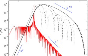
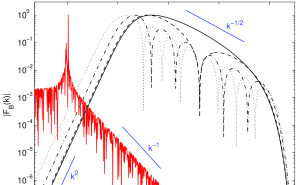
Figure 2: Absolute values of magnetic energy spectral eigenfunctions for four selected bound eigenmodes (shown by the dotted, dash-dot, dashed and smooth solid lines), and for the fastest growing unbound eigenmode (shown by the red jagged spiky solid lines). All plots are for $\eta=10^{-12}$ (${\rm Rm}\sim 10^{12}$). The left and right plots are for the cases $h=1$ and $h=0.01$ respectively.

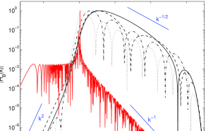
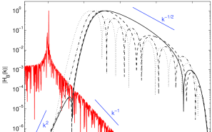
Figure 3: The same as figure 2 except the absolute values of electric current helicity spectral eigenfunctions are plotted here.

In the case ${\rm Rm}\sim 10^{6}$ and $h=1$ there exist four bound magnetic field eigenmodes. They have growth rates $\lambda_{1}\simeq 0.9991$, $\lambda_{2}\simeq 1.669$, $\lambda_{3}\simeq 2.681$ and $\lambda_{4}\simeq 3.443$, which are shown on the plot A in figure 1. The fastest growing unbound eigenmode grows at a rate $\lambda_{0}\simeq 0.9943$. In the case ${\rm Rm}\sim 10^{6}$ and $h=0.01$ the number of bound eigenmodes is again four, $\lambda_{1}\simeq 0.1750$, $\lambda_{2}\simeq 1.507$, $\lambda_{3}\simeq 2.629$ and $\lambda_{4}\simeq 3.430$, while the fastest growing unbound eigenmode is $\lambda_{0}\simeq 9.943\times 10^{-5}$, refer to the plot B in figure 1. Next, in the case ${\rm Rm}\sim 10^{12}$ and $h=1$ there are seven bound eigenmodes, all shown on the plot C in figure 1. Among these we select four bound modes $\lambda_{1}\simeq 1.192$, $\lambda_{3}\simeq 2.322$, $\lambda_{6}\simeq 3.499$, $\lambda_{7}\simeq 3.686$, and we plot their spectral eigenfunctions by the dotted, dash-dot, dashed and smooth solid lines respectively on the left plots in figures 2 and 3. The spectral eigenfunctions of the fastest unbound mode $\lambda_{0}\simeq 0.9943$ are shown by the red jagged spiky lines on these left plots. Finally, in the case ${\rm Rm}\sim 10^{12}$ and $h=0.01$ there are eight bound eigenmodes, refer to plot D in figure 1. The spectral eigenfunctions of four selected bound modes $\lambda_{1}\simeq 0.2948$, $\lambda_{3}\simeq 1.694$, $\lambda_{7}\simeq 3.494$ and $\lambda_{8}\simeq 3.685$ are shown by the dotted, dash-dot, dashed and smooth solid lines on the right plots in figures 2 and 3. The spectra of the fastest unbound mode $\lambda_{0}\simeq 9.943\times 10^{-5}$ are again shown by the red jagged spiky lines. As an interesting result, note that in figures 2 and 3 the envelopes of all bound eigenfunctions – not only the envelope of the fastest growing eigenfunction – agree with the Kazantsev spectral slope $k^{-1/2}$ (compare to Kulsrud and Anderson 1992).

Using the results presented in figures 1–3, we make the following conclusions. First, the value of kinetic helicity parameter $h$ does not have much effect on the fastest growing bound eigenmodes (e.g., compare modes $\lambda_{5}$, $\lambda_{6}$, $\lambda_{7}$ on plot C to modes $\lambda_{6}$, $\lambda_{7}$, $\lambda_{8}$ on plot D in figure 1), but it does influence the unbound eigenmodes. This result is expected because helicity of velocity fluctuations does not propagate to small scales (Kulsrud and Anderson 1992), however, $\lambda_{0}=g^{2}(0)/[\kappa_{L}(0)+2\eta]\sim h^{2}v_{0}/l_{0}$. Second, at a fixed kinetic helicity value, when the magnetic Reynolds number increases, the number of bound modes increases (refer to figure 1). This is also expected because, the diffusion of magnetic field decreases with an increase of the magnetic Reynolds number. Third, let us refer to the spectra of the fastest growing unbound eigenmodes $\lambda_{0}$, which are shown by the the red jagged spiky solid lines in figures 2 and 3. We see that when the value of the kinetic helicity drops by a factor of a hundred (from $h=1$ to $h=0.01$), the location of the peaks of these spectra shifts to larger scales by the same factor. Thus, the characteristic scale of eigenmode $\lambda_{0}$ is approximately equal to $\sim l_{0}/h$, and this mode becomes large-scale when kinetic helicity is small, in agreement with the physical picture of large-scale dynamo action (Steenbeck et al. 1966). 

We thank Fausto Cattaneo for useful discussions. This work was supported by the NSF Center for Magnetic Self-Organization in Laboratory and Astrophysical Plasmas. SB is supported by the U.S. Dept. of Energy under the grant No. DE-FG02-07ER54932.

References

References

- [1] [] Boldyrev, S., Cattaneo, F., and Rosner, R. 2005, Phys. Rev. Lett., 95, 255001
- [2] [] Brandenburg, A., and Subramanian, K. 2005, Phys. Rep., 417, 1
- [3] [] Kazantsev, A. P. 1968, JETP, 26, 1031
- [4] [] Kim, E., and Hughes, D. W. 1997, Phys. Lett. A, 236, 211
- [5] [] Kraichnan, R. H., Phys. Fluids 1968, 11, 945
- [6] [] Kulsrud, R. M. 2005, Plasma Physics for Astrophysics (Princeton University Press)
- [7] [] Kulsrud, R. M., and Anderson, S. W. 1992, Astrophys. J., 396, 606
- [8] [] Kulsrud, R. M., and Zweibel, E. G. 2008, Rep. Prog. Phys., 71, 046901
- [9] [] Lynden-Bell, D. (ed.) 1994, Cosmical Magnetism (Dordrecht: Kluwer Academic Publishers)
- [10] [] Malyshkin, L., and Boldyrev, S. 2007, Astrophys. J. Lett., 671, L185
- [11] [] Moffatt, H. K. 1978, Magnetic Field Generation in Electrically Conducting Fluids (Cambridge U. Press)
- [12] [] Monin, A. S., and Yaglom, A. M. 1971, Statistical Fluid Mechanics (MIT Press)
- [13] [] Parker, E. N. 1979, Cosmical Magnetic Fields (Oxford: Clarendon Press)
- [14] [] Steenbeck, M., Krause, F., and Radler, K. H. 1966, Z. Naturforsch., 21a, 369
- [15] [] Vainshtein, S. I., and Kichatinov, L. L. 1986, J. Fluid Mech., 168, 73
- [16] [] Vainshtein, S. I., and Zeldovich, Ya. B. 1972, Sov. Phys. Uspekhi, 15, 159
- [17] [] Zweibel, E. G., and Heiles, C. 1997, Nature, 385, 131