Quantum entanglement of space domains occupied by interacting electrons

Abstract

Spin-entanglement of two electrons occupying two spatial regions – domains – is expressed in a compact form in terms of spin-spin correlation functions. The power of the formalism is demonstrated on several examples ranging from generation of entanglement by scattering of two electrons to the entanglement of a pair of qubits represented by a double quantum dot coupled to leads. In the latter case the collapse of entanglement due to the Kondo effect is analyzed.

1 Introduction

Based on the peculiar behaviour of entangled quantum states, in 1935 Einstein, Podolsky and Rosen argued that quantum mechanical description of reality is not complete [1]. Today this article is Einstein’s most cited publication, but quantum entanglement is not considered a paradox. In fact, the ability to establish entanglement between quantum particles in a controlled manner is a crucial ingredient of any quantum information processing system [2]. Also, the study of entanglement provides insight into the nature of many-body states in the vicinity of crossovers between various regimes or points of quantum phase transition [3].

In realistic hardware designed for quantum information processing, several criteria for qubits (DiVincenzo’s checklist) must be fulfilled [4]: the existence of multiple identifiable qubits, the ability to initialize and manipulate qubits, small decoherence, and the ability to measure qubits, i.e., to determine the outcome of computation. Quite generally, the parts of an interacting system are to some extent entangled. However, fully entangled qubit pairs are required for such applications [2]. This leads to the question of how to quantify the entanglement.

The entanglement of binary quantum objects (qubits) can be quantified by the entanglement of formation, a notion which for pure states reduces to the von Neumann entropy [5, 6, 7]. This measure is convenient since it is proportional to the number of fully entangled pairs needed to produce a given entangled state. Also, it is monotonically related to the concurrence, which can be evaluated by the Wootters formula [8] as a simple function of the density matrix.

A possible realization of a qubit pair can be achieved by confining electrons to two spatial regions. In this case one has the freedom to choose between spin or charge of the electron to represent a qubit. The entanglement measures must account for both possibilities. Additional complications arise due to the indistinguishability of the particles and possible states of multiple occupancy [9, 10, 11, 12].

On the experimental side, it seems that among several proposals for quantum information processing systems, the criteria for scalable qubits can be met in solid state structures consisting of coupled quantum dots [13, 14]. The ability to precisely control the number of electrons [15] and the evidence for spin entangled states have been reported in GaAs based heterostructures [16, 17]. It has also been demonstrated that in double quantum dot systems coherent qubit manipulation and projective readout are possible [18].

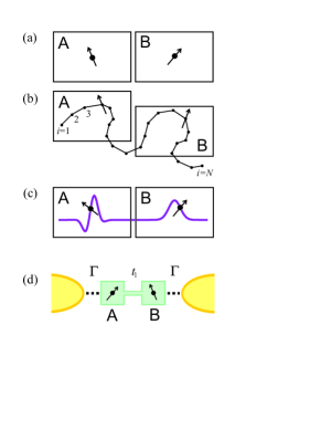
Figure 1: (Color online) (a) Two electrons (qubits) localized in separate quantum dots A and B. (b) Two delocalized electrons in separate measurement domains A and B; the probability of finding one electron in a domain is equal for A and B: $n_{A}=n_{B}=1$. (c) Scattering of two electrons. (d) Double quantum dot system coupled to the leads: the chemical potential is set such that each of the dots is occupied by one interacting electron on average.

Here we explicitely evaluate the concurrence in terms of spin-spin correlation functions between the two subsystems. In this manner we easily account for entanglement between subsystems containing delocalized electrons. We demonstrate the convenience of our approach by evaluating the time-dependence of concurrence in a toy example of two electrons in a three site chain and in a more realistic entangler based on scattering of electrons in a quantum wire.

On the other hand, entangled qubits can also be extracted from interacting many-body systems. Our formulas are readily generalized also for this case and even for finite temperature. As an example, we discuss the case of two quantum dots coupled serially to metallic electrodes. In this case, entanglement of a pair of electrons that are confined in a double quantum dot may collapse at low temperatures due to the Kondo effect even for a very weak coupling to the leads.

The paper is organized as follows. Sec. 2 introduces the entanglement measure for two delocalized electrons, which can be simplified for some special cases elaborated in Sec. 3. In Sec. 4 we illustrate the convenience of our approach with numerical examples mentioned above. Conclusions are given in Sec. 5.

2 Entanglement of two delocalized electrons

A pure state of two spins represented by electrons, each occupying a separate quantum dot $A$ and $B$, can be described in the basis of single spin-$\frac{1}{2}$ states $s=\uparrow$ or $\downarrow$ as $|\Psi_{AB}\rangle=\sum_{ss^{\prime}}\alpha_{ss^{\prime}}|s\rangle_{\!A}|s^{\prime}\rangle_{\!B}$. Such a state, Fig. 1(a), is factorizable $|\Psi_{AB}\rangle=|\phi_{A}\rangle|\phi_{B}\rangle$ if and only if $\alpha_{\uparrow\!\downarrow}\alpha_{\downarrow\!\uparrow}=\alpha_{\uparrow\!\uparrow}\alpha_{\downarrow\!\downarrow}$ as easily checked by explicit construction. For general coefficients $\alpha_{ss^{\prime}}$ the state is not factorizable and its entanglement can be quantified by concurrence $C$ as introduced by Hill and Wootters [6],

$$C=2|\alpha_{\uparrow\!\downarrow}\alpha_{\downarrow\!\uparrow}-\alpha_{\uparrow\!\uparrow}\alpha_{\downarrow\!\downarrow}|.$$ (1)

Consider now a more general problem of two electrons in a state where the system cannot directly be reduced to an equivalent system with (pseudo) spin degrees of freedom only. Let us take for example two electrons on a lattice [19] described by a state

$$|\Psi\rangle=\sum_{(i,j)\;ss^{\prime}}\psi_{ij}^{ss^{\prime}}c_{is}^{\dagger}c_{js^{\prime}}^{\dagger}|0\rangle,$$ (2)

where $c_{is}^{\dagger}$ creates an electron with spin $s$ on site $i$ on the lattice with the total number of sites $N$. Sites of the lattice are assumed to be ordered as for example in Fig. 1(b) and $(i,j)$ corresponds to the summation over all sites $i=1,...N$ and $i\leq j$ [20].

Such states may arise when two initially unentangled electrons in wave packets approach each other, then interact and finally become again well separated in distinct regions A and B, Fig. 1(c), where they could be extracted for further purposes. Alternatively, such states can be realized in various correlated electron systems and, in order to study them theoretically, elaborate many-body techniques are sometimes needed. Moreover, usually not the state itself but only the correlation functions are available.

Therefore it is advantageous to express the entanglement in terms of spin-spin correlation functions. The spin operators for a single electron occupying domain A (or B) are expressed as the sum of operators for sites $i$ within the given domain,

$$S_{A(B)}^{\lambda}=\frac{1}{2}\sum_{i\in A(B)}\sum_{ss^{\prime}}c_{is}^{\dagger}\sigma_{ss^{\prime}}^{\lambda}c_{is^{\prime}},$$ (3)

where $\sigma^{\lambda}_{ss^{\prime}}$ are the Pauli matrices.

The concurrence is given by the eigenvalues of the non-Hermitian matrix $\rho\tilde{\rho}$, where $\rho$ and $\tilde{\rho}$ are the reduced density matrix and its time reverse, respectively [8]. For axially symmetric problems, where both $\langle\Psi|S_{A(B)}^{x}|\Psi\rangle=0$ and $\langle\Psi|S_{A(B)}^{y}|\Psi\rangle=0$ as well as $\langle\Psi|S_{A(B)}^{z}S_{B(A)}^{x}|\Psi\rangle=0$ and $\langle\Psi|S_{A(B)}^{z}S_{B(A)}^{y}|\Psi\rangle=0$, it can be expressed in a compact form [19]

$$C = \textrm{max}(0,C_{\uparrow\!\downarrow},C_{\parallel}),$$ (4)

$$C_{\uparrow\!\downarrow} = 2|\langle S_{A}^{+}S_{B}^{-}\rangle|-2\sqrt{\langle P_{A}^{\uparrow}P_{B}^{\uparrow}\rangle\langle P_{A}^{\downarrow}P_{B}^{\downarrow}\rangle},$$

$$C_{\parallel} = 2|\langle S_{A}^{+}S_{B}^{+}\rangle|-2\langle P_{A}^{\uparrow}P_{B}^{\downarrow}\rangle,$$

where $S_{A(B)}^{+}=(S_{A(B)}^{-})^{\dagger}=\sum_{i\in A(B)}c_{i\uparrow}^{\dagger}c_{i\downarrow}$ are spin raising operators for domains A (or B) and

$$P_{A(B)}^{s}=\sum_{i\in A(B)}n_{is}(1-n_{i,-s})$$ (5)

are spin-$s$ projectors operating in domains A (or B) with $n_{is}=c_{is}^{\dagger}c_{is}$. Fermionic expectation values required in Eq. (4) are then given as

$$\langle S_{A}^{+}S_{B}^{-}\rangle = \sum_{[ij]}\psi_{ij}^{\uparrow\!\downarrow*}\psi_{ij}^{\downarrow\!\uparrow},$$

$$\langle S_{A}^{+}S_{B}^{+}\rangle = \sum_{[ij]}\psi_{ij}^{\uparrow\!\uparrow*}\psi_{ij}^{\downarrow\!\downarrow},$$ (6)

$$\langle P_{A}^{s}P_{B}^{s^{\prime}}\rangle = \sum_{[ij]}|\psi_{ij}^{ss^{\prime}}|^{2},$$

where $[ij]$ in Eqs. (6) corresponds to the summation over all pairs $i,j$ such that $i\in A$ and $j\in B$. Concurrence formula Eq. (4) is valid as long as double occupancy of sites is negligible, $\langle n_{is}n_{is^{\prime}}\rangle\to 0$. It is assumed that the wave function is normalized,

$$\langle\Psi|\Psi\rangle=\sum_{(i,j),\;ss^{\prime}}|\psi_{ij}^{ss^{\prime}}|^{2}=1.$$ (7)

We stress that the correlation functions in Eq. (4) can be evaluated for pure or mixed states, the latter arising, for instance, due to the finite temperature or by tracing out the environment degrees of freedom, e.g., leads in Fig. 1(d).

3 Special cases

In states with the SU(2) symmetry $\langle S_{A}^{x}S_{B}^{x}\rangle=\langle S_{A}^{y}S_{B}^{y}\rangle=\langle S_{A}^{z}S_{B}^{z}\rangle$ and the concurrence formula Eq. (4) simplifies further to a function depending on only one spin invariant $\langle\textrm{\bf S}_{\mathrm{A}}\cdot\textrm{\bf S}_{\mathrm{B}}\rangle$,

$$C_{\mathrm{A}\mathrm{B}}=\textrm{max}\left(0,-2\langle\textrm{\bf S}_{\mathrm{A}}\cdot\textrm{\bf S}_{\mathrm{B}}\rangle-\frac{1}{2}\right).$$ (8)

The concurrence is expected to be significant whenever enhanced spin-spin correlations indicate A-B singlet formation.

If $|\Psi\rangle$ is an eigenstate of the total spin projection $S_{\textrm{tot}}^{z}$ the concurrence is given solely with the overlap between $|\Psi\rangle$ and the $AB$-spin-flipped state $|\tilde{\Psi}\rangle=|S_{A}^{+}S_{B}^{-}\Psi\rangle$. If $S_{\textrm{tot}}^{z}=\pm 1$ the concurrence is zero, while for $S_{\textrm{tot}}^{z}=0$

$$C=C_{\uparrow\!\downarrow}=2|\sum_{[ij]}\psi_{ij}^{\uparrow\!\downarrow*}\psi_{ij}^{\downarrow\!\uparrow}|,$$ (9)

which is a generalization of the concurrence formula Eq. (1) to $N$ sites.

The concurrence formulas, Eq. (4), remain essentially the same if the state $|\Psi\rangle$ corresponds to the system in continuum space, $i\rightarrow{\textbf{r}}=(x,y,z)$, the only change being integrations over the corresponding measurement domains,

$$C=|\int_{A}\!\int_{B}\!(\varphi_{0}\!-\varphi_{1})^{*}(\varphi_{0}\!+\varphi_{1})\textrm{d}^{3}{\textbf{r}}_{1}\textrm{d}^{3}{\textbf{r}}_{2}|,$$ (10)

where $\varphi_{S}\equiv\varphi_{S}(\textbf{r}_{1},{\textbf{r}_{2})=\langle{\textbf{r}}_{1},{\textbf{r}}_{2};S}|\Psi\rangle$ are singlet and triplet amplitudes for $S=0$ and $S=1$, respectively.

Another interesting special case is the wave function $|\Psi\rangle$ which is a linear combination of entangled Bell $AB$-pairs,

$$|\Psi\rangle=\sum_{\beta=1}^{4}b_{\beta}\sum_{[ij]}\psi_{ij}|ij,\beta\rangle,\,\,\,\,\,\sum_{[ij]}|\psi_{ij}|^{2}=1,$$ (11)

where for each pair of sites $(i,j)$ one can introduce the Bell basis $|ij,\beta\rangle$ [5],

$$|ij,1\rangle = \frac{1}{\sqrt{2}}(c_{i\uparrow}^{\dagger}c_{j\uparrow}^{\dagger}+c_{i\downarrow}^{\dagger}c_{j\downarrow}^{\dagger})|0\rangle,$$ (12)

$$|ij,2\rangle = \frac{\imath}{\sqrt{2}}(c_{i\uparrow}^{\dagger}c_{j\uparrow}^{\dagger}-c_{i\downarrow}^{\dagger}c_{j\downarrow}^{\dagger})|0\rangle,$$

$$|ij,3\rangle = \frac{\imath}{\sqrt{2}}(c_{i\uparrow}^{\dagger}c_{j\downarrow}^{\dagger}+c_{i\downarrow}^{\dagger}c_{j\uparrow}^{\dagger})|0\rangle,$$

$$|ij,4\rangle = \frac{1}{\sqrt{2}}(c_{i\uparrow}^{\dagger}c_{j\downarrow}^{\dagger}-c_{i\downarrow}^{\dagger}c_{j\uparrow}^{\dagger})|0\rangle.$$

In this case, the concurrence is given with a simple expression $C=|\sum_{\beta}b_{\beta}^{2}|$.

4 Numerical examples

Here we use concurrence formulas in practice. We evaluate the concurrence for a few examples of interacting electrons on a lattice described by the following generic hamiltonian

$$H=-\sum_{ijs}(t_{ij}c_{is}^{\dagger}c_{js}+h.c.)+\sum_{ijss^{\prime}}U_{ij}n_{is}n_{js^{\prime}}.$$ (14)

For simplicity we take the electron-electron interaction constant up to some distance, i.e., $U_{ij}=\frac{1}{2}U\sum_{m=0}^{M}\delta_{|i-j|,m}$.

Figure 2: (Color online) Full line represents concurrence $C(t)$ for a three sites system with $t_{12}/t_{23}=1/10$, $U/t_{23}=5$ and $J_{\textrm{eff}}/t_{23}=0.023$ (singlet-triplet energy difference). Dashed line corresponds to the strong coupling limit results $C_{\textrm{eff}}(t)$ with the same $J_{\textrm{eff}}$. Domains are doubly occupied with the probability $P_{2}$.

4.1 Two qubits on three sites

First we consider two electrons on three sites, where site $i=1$ corresponds to the measuring domain A and sites $i=2,3$ to the domain B. We take the Hubbard model, $M=0$, and two non-zero hopping matrix elements, $t_{12}$ and $t_{23}$. In the limit $t_{23}>t_{12}$ a bonding orbital is formed between the sites 2 and 3 and in the ground state of the system there is a single electron in each of the domains. For large $U$, the ground state is a spin singlet formed between site $i=1$ and the bonding orbital, with the excitation energy $J$ to the triplet state.

If in each of the domains there is precisely one electron and the state is an eigenstate of total spin projection, $S_{\textrm{tot}}^{z}=0$, Eq. (4) simplifies to

$$C=2|\psi_{12}^{\uparrow\!\downarrow*}\psi_{12}^{\downarrow\!\uparrow}+\psi_{13}^{\uparrow\!\downarrow*}\psi_{13}^{\downarrow\!\uparrow}|.$$ (15)

Let us put the electrons to the system in an initially separable state consisting of a spin up electron in A and the other electron with spin down in the bonding orbital of B, $|\Psi(0)\rangle=c^{\dagger}_{1\uparrow}{1\over\sqrt{2}}(c^{\dagger}_{2\downarrow}+c^{\dagger}_{3\downarrow})|0\rangle$. Because the inital state is composed of different energy eigen-states, the Rabi oscillations occur. In the strong coupling limit, $U,t_{23}\gg t_{12}$ the system is described by the Heisenberg model with antiferromagnetic coupling $J_{\textrm{eff}}\sim 8t_{12}^{2}/(U-2t_{23})$ between the site 1 and the bonding orbital. In this limit the Rabi oscillations occur due to the singlet-triplet splitting and the time evolution of concurrence is given by $C_{\textrm{eff}}=|\sin J_{\textrm{eff}}t|$.

For generic values of parameters additional states, for example the states when the site 1 is doubly occupied, become relevant. We show the concurrence for such a case in Fig. 2 and compare it to the simplified expression given above. The simple behaviour is partly reproduced but additional oscilations arise on other time scales. We plot also the probability that both electrons simultaneously occupy one of the domains, $P_{2}=1-\langle n_{1\uparrow}+n_{1\downarrow}\rangle+2\langle n_{1\uparrow}n_{1\downarrow}\rangle$. The oscillations of this quantity occur on the time scale given by the characteristic time of tunneling events, $t_{12}^{-1}$.

4.2 Two flying qubits

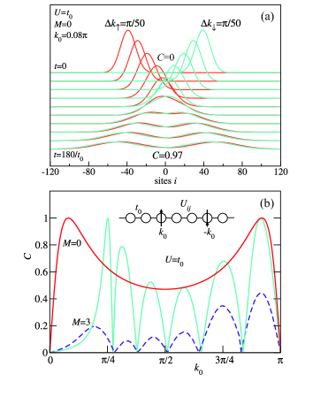
Figure 3: (Color online) (a) Time evolution of spin $\uparrow$ and $\downarrow$ electron density during the scattering for the Hubbard model $(M=0)$ with $U=t_{0}$ and $\Delta k=\pi/50$ and $k_{0}$ near the concurrence maximum. (b) $C$ as a function of $k_{0}$: (i) the Hubbard model $(M=0)$ with $U=t_{0}$ and $\Delta k=0$; (ii) $M=3$: with $\Delta k=0$ (full line), and (iii) $\Delta k=\pi/10$ (dashed).

Next we consider two flying qubits, i.e., two electrons on an infinite one-dimensional lattice with the hamiltonian Eq. (14) and $t_{ij}=t_{0}$ for $j=i+1$. To be specific, let one electron with spin $\uparrow$ be confined initially to region $A$ ($i\sim-L$) and the other electron with opposite spin to region $B$ ($i\sim L)$, Fig. 3. The simplest initial state consists of two wave packets with vanishing momentum uncertainties $\Delta k\rightarrow 0$, with momenta $k>0$ and $q<0$ for the left and the right wave packet, respectively. After the collision, the electrons move apart with a probability amplitude ${\cal M}_{||}(k,q)$ for non-spin-flip scattering and a spin-flip amplitude ${\cal M}_{\uparrow\!\downarrow}(k,q)$. Concurrence after the collision is then readily expressed from Eq. (9) as

$$C=2|{\cal M}_{||}(k,q){\cal M}_{\uparrow\!\downarrow}(k,q)|.$$ (16)

Note that $C=1$ when non-spin-flip and spin-flip amplitudes coincide in accord with recent analysis of flying and static qubits entanglement [21, 22, 23, 24].

More general initial wave packets with finite $\Delta k$ are defined with appropriate momentum amplitudes $\phi_{\uparrow}(k)$ and $\phi_{\downarrow}(q)$ for spin $\uparrow$ and $\downarrow$, respectively. The concurrence as follows from Eq. (9)

$$C=2|\int\!\!\!\int{\cal M}_{||}^{*}(k,q){\cal M}_{\uparrow\!\downarrow}(k,q)|\phi_{\uparrow}(k)\phi_{\downarrow}(q)|^{2}\textrm{d}k\textrm{d}q|$$ (17)

consists of a coherent superposition of scattering amplitudes [19].

The simplest example is the Hubbard model where the scattering amplitudes can be obtained analytically for the case of one-dimension, ${\cal M}_{||}(k,q)=1+{\cal M}_{\uparrow\!\downarrow}(k,q)=(\sin k-\sin q)/[\sin k-\sin q+\imath U/(2t_{0})]$ [25]. In Fig. 3(a) the time evolution of spin $\uparrow$ and $\downarrow$ electron densities is presented. In Fig. 3(b) the corresponding concurrence for wave packets with a well defined momentum $k_{0}$ for $U=t_{0}$ is shown, together with a longer range interaction case, $M=3$, for a sharp momentum (full line) and for a Gaussian initial amplitude $\phi_{\downarrow}(q)=\phi_{\uparrow}(-k)$ with $\Delta k=\pi/10$ (dashed line). An interesting observation here is a substantial reduction of the concurrence due to coherent averaging in Eq. (17). Additionally, electrons will be completely entangled at some kinetic energy comparable with the repulsion, $U\sim 2t_{0}(1-\cos k_{0})$, where non-spin-flip and spin-flip amplitudes coincide. In Fig. 4(a) and Fig. 5(a) some representative additional examples of time evolution of interacting wave packets are shown.

The concurrence formula Eq. (9) is derived for electronic states when double occupancy is negligible, which in our case is strictly fulfilled only asymptotically when the electrons are far apart. However, Eq. (9) can be evaluated at any time $t$ and the resulting $C(t)$ can serve as a measure of entanglement during the transition from initial to final state. In Fig. 4(b) and Fig. 5(b) $C(t)$ corresponding to parameters of Fig. 4(a) and Fig. 5(a) is shown. Concurrence oscillations can be interpreted as a response to the finite time duration of electron-electron interaction – exchange – where the model can be approximately mapped onto an effective Heisenberg model as in the case of three sites presented above.

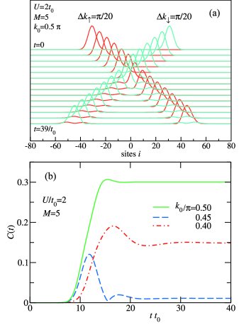
Figure 4: (Color online) (a) Time evolution of spin $\uparrow$ and $\downarrow$ electron density for $U=2t_{0}$, $M=5$ with $k_{0}=0.5\pi$, $\Delta k_{\uparrow}=\Delta k_{\downarrow}=\pi/20$. (b) $C(t)$ for Gaussian packets with various $k_{0}$, $M=5$, $U=2t_{0}$ and $\Delta k=\pi/20$. At $t=0$ the separation between the packets is $2L=10/\Delta k$.

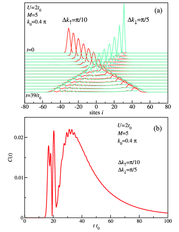
Figure 5: (Color online) As in Fig. 4, with parameters $U=2t_{0}$, $M=5$ but different $k_{0}=0.4\pi$, $\Delta k_{\uparrow}=\pi/10$ and $\Delta k_{\downarrow}=\pi/5$.

4.3 Qubit pairs in coupled quantum dots

One of the simplest realizations of a solid state qubit is a serially coupled double quantum (DQD). We model such a DQD using the two-impurity Anderson Hamiltonian

$$H = \sum_{i=\mathrm{A},\mathrm{B}}(\epsilon n_{i}+Un_{i\uparrow}n_{i\downarrow})+Vn_{\mathrm{A}}n_{\mathrm{B}}$$

$$-t_{1}\sum_{s}(c_{\mathrm{A}s}^{\dagger}c_{\mathrm{B}s}+h.c.),$$

where $c^{\dagger}_{is}$ creates an electron with spin $s$ in the dot $i=\mathrm{A}$ or $i=\mathrm{B}$ and $n_{is}=c^{\dagger}_{is}c_{is}$ is the number operator. The on-site energies $\epsilon$ and the Hubbard repulsion $U$ are taken equal for both dots. The dots are coupled to the left and right noninteracting tight-binding leads with the chemical potential set to the middle of the band of width $4t_{0}$. Each of the dots is coupled to the adjacent lead by hopping $t_{2}$ and the corresponding hybridization width is $\Gamma=(t_{2})^{2}/t_{0}$. Schematically this setup is presented in Fig. 1(d). The dots are additionally coupled capacitively by a inter-dot repulsion term $Vn_{\mathrm{A}}n_{\mathrm{B}}$.

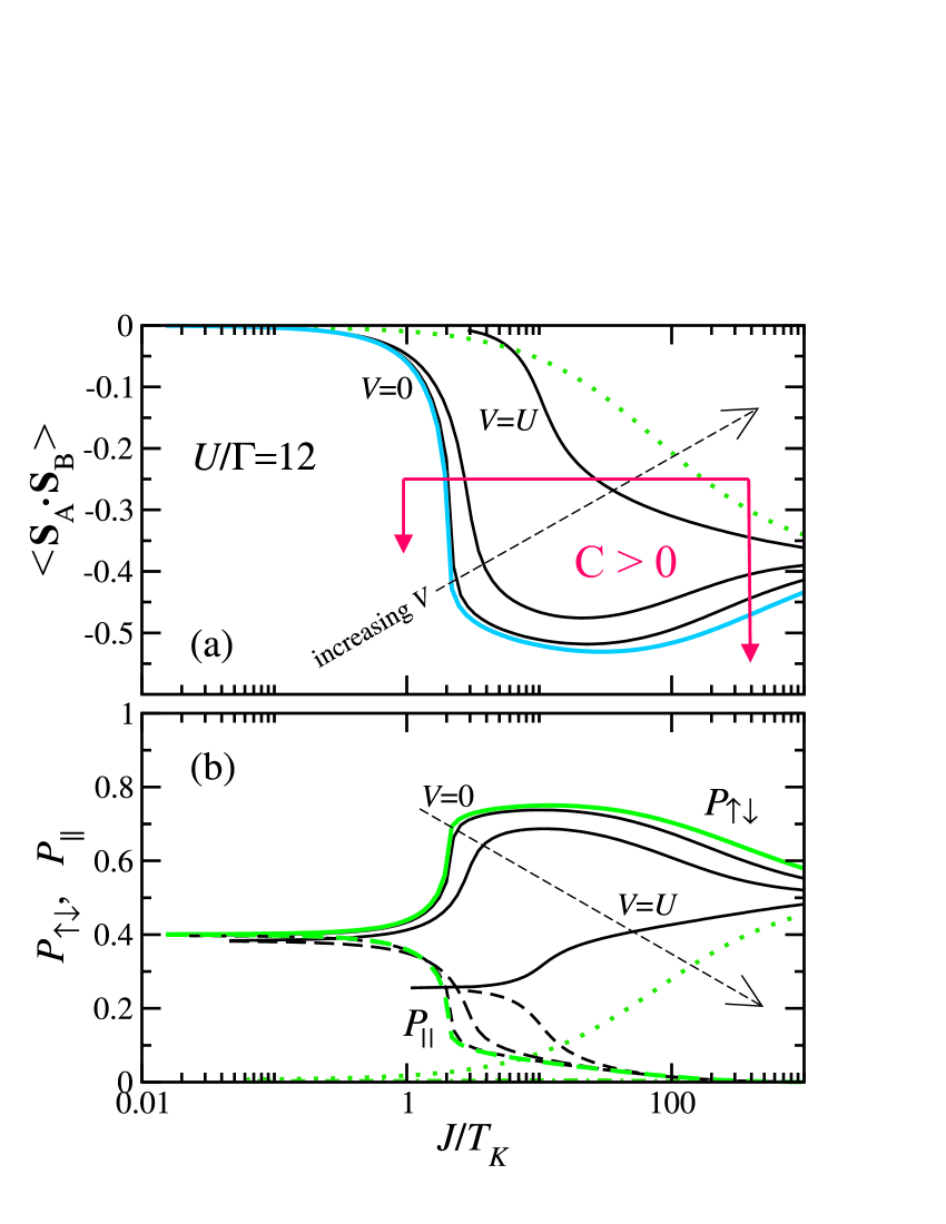
Figure 6: (a) Spin-spin correlation for $V/U=0,1/3,2/3,1$ (full lines) and $V/U=5/4$ (dotted) for $U/\Gamma=12,\Gamma/t_{0}=0.1$. (b) Probabilities for parallel (lower curves - dashed) and anti-parallel (upper curves - full) spins of electrons in the DQD for $V/U$ ratios as in (a). Note that the probability for parallel spins for $V/U=5/4$ is almost zero (dashed-dotted), while $P_{\uparrow\downarrow}<1/2$ for $J/T_{K}<1000$ (dotted); the probabilities do not sum to 1. The deficiency (which goes to zero as $U\to\infty$) is due to the states with double occupancy on at least one of the dots.

When a DQD is attached to leads the low temperature physics is to a large extent the same as that of the two-impurity Kondo problem [26]. There two impurities form either two Kondo singlets with delocalized electrons or bind into a local spin-singlet state which is virtually decoupled from delocalized electrons. The crossover between the regimes is determined by the relative values of the exchange magnetic energy $J$ and twice the Kondo condensation energy, of order the Kondo temperature given by the Haldane formula, $T_{K}=\sqrt{U\Gamma/2}\exp(-\pi\epsilon(\epsilon+U)/2\Gamma)$. The competition between extended Kondo and local-singlet states occurs rather generally in systems of coupled quantum impurities [27, 28, 29].

A qubit pair represented by two electrons in a DQD and in the contact with the leads acting as a fermionic bath can not be described by a pure state. In the case of mixed states of qubit pairs as studied here the concurrence is related to the reduced density matrix of the DQD subsystem as in the previous case of delocalized electrons pairs. If $t_{1(2)}/U$ is not small the electrons can fluctuate between the dots (and to the leads) and such charge fluctuations introduce additional states with zero or double occupancy of individual dots [9, 11]. As pointed out by Zanardi in the case of simple Hubbard dimer [11] the entanglement is not related only to spin but also to charge degrees of freedom which emerge when repulsion between electrons is weak or moderate.

For systems with strong electron-electron repulsion considered here, charge fluctuations are suppressed and the states with single occupancy – the spin-qubits – dominate and the concept of spin-entanglement quantified with concurrence can be applied. We again use spin-projected density matrix and consider only entanglement corresponding to spin degrees of freedom. Due to doubly (or zero) occupied states arising from charge fluctuation on the dots (caused by tunneling between the dots A and B or due to the exchange with the electrons in the leads), the reduced density matrix has to be renormalized. The probability that at the measurement of entanglement there is precisely one electron on each of the dots is less than unity, $P_{11}<1$, and the spin-concurrence is then given with

$$C_{11}=C/P_{11},$$ (19)

where $P_{11}=P_{\uparrow\downarrow}+P_{\parallel}$, and $P_{\uparrow\downarrow}=\langle P^{\uparrow}_{\mathrm{A}}P^{\downarrow}_{\mathrm{B}}+P^{\downarrow}_{\mathrm{A}}P^{\uparrow}_{\mathrm{B}}\rangle$, $P_{\parallel}=\langle P^{\uparrow}_{\mathrm{A}}P^{\uparrow}_{\mathrm{B}}+P^{\downarrow}_{\mathrm{A}}P^{\downarrow}_{\mathrm{B}}\rangle$ are probabilities for antiparallel and parallel spin alignment, respectively. Such a procedure corresponds to the measurement apparatus which would only discern spins and ignore all cases whenever no electron, or a electron pair would appear at one of the detectors at sites A or B.

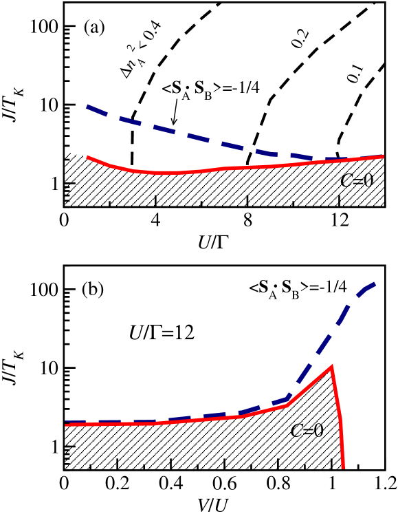
Figure 7: (a) Charge fluctuations of the domain A, $\Delta n_{A}^{2}=\langle n_{A}^{2}\rangle-\langle n_{A}\rangle^{2}$ (short-dashed), $\langle\textrm{\bf S}_{A}\cdot\textrm{\bf S}_{B}\rangle=-1/4$ (long-dashed) and $C=0$ (full) in the $(U/\Gamma,J/T_{K})$ plane. (b) $\langle\textrm{\bf S}_{A}\cdot\textrm{\bf S}_{B}\rangle=-1/4$ (long-dashed) and $C=0$ (full) in the $(V/U,J/T_{K})$ plane.

Here we present results for the zero temperature limit obtained by the projection operator method as in Refs. [30, 31, 32, 33, 34]. The temperature dependence of the concurrence for the case of $V=0$ is given in Ref.  [35]. Expectation values $\langle...\rangle$ in the concurrence formula Eq. (4) are now calculated using the ground state therefore $\langle S_{\mathrm{A}}^{+}S_{\mathrm{B}}^{+}\rangle=0$ and $C_{\parallel}<0$. We consider the particle-hole symmetric point with $n=2$ and $\epsilon+U/2+V=0$.

Qualitatively, the concurrence is significant whenever enhanced spin-spin correlations indicate inter-dot singlet formation. As shown in Fig. 6(a) for $U/\Gamma=12$ and $\Gamma/t_{0}=0.1$, the correlation function $\langle{\bf S}_{\mathrm{A}}\cdot{\bf S}_{\mathrm{B}}\rangle$ tends to $-3/4$ for $J$ large enough to suppress the formation of Kondo singlets, but still $J/U\ll 1$, that local charge fluctuations are sufficiently suppressed. In particular, the local dot-dot singlet is formed whenever singlet-triplet splitting superexchange energy $J>J_{c}\sim 2T_{K}$. With increasing $V\to U$, and above $U$, the probability for singly occupied spin states, $P_{11}=P_{\uparrow\downarrow}+P_{\parallel}$ is significantly reduced, Fig. 6(b), which also leads to reduced spin-spin correlation.

The entanglement between qubits quantified by concurrence is small in the regime where the Kondo effect determines the ground state. The Kondo screening transfers the entanglement between localized electrons to the mutual entanglement of localized and the conducting electrons [36]. For $V\sim U$ the Kondo temperature is enhanced and the corresponding Kondo ground state is competitive towards the localized singlet state. In Fig. 7(a) we present a phase diagram of regions with finite and zero entanglement, separated approximately by the $J\sim 2T_{K}$ line. In the strong coupling limit the boundary coincides with the $\langle\textrm{\bf S}_{A}\cdot\textrm{\bf S}_{B}\rangle=-1/4$ dashed line. For $V>U+T_{K}$ the Kondo screening is inhibited and the concurrence is increased, Fig. 7(b). However, the probability for doubly occupied sites is not small in this regime and the concept of spin-qubits is not appropriate there [31].

5 Conclusion

In this work we showed that the applicability of the concurrence, an entanglement measure originally restricted to two distinguishable particles (spins), can be extended to two regions – measurement domains – occupied by two indistinguishable particles (electrons). The proposed approach allows for the analysis of entanglement in a variety of realistic problems, from scattering of flying and static qubits, the former being represented as wave packets with a finite energy resolution, to the time evolution of static qubits due to electron-electron interaction or externally applied fields. A generalization to systems described as a mixed state and containing more than two electrons is possible. As an example, a double quantum dot system occupied, on average, by two interacting electrons is presented.

We acknowledge support from the Slovenian Research Agency under contract Pl-0044.

References

- [1] A. Einstein, B. Podolsky, and N. Rosen, Phys. Rev. 47, 777 (1935).
- [2] M. A. Nielsen and I. A. Chuang, Quantum Information and Quantum Computation (Cambridge University Press, Cambridge, 2001).
- [3] A. Osterloh, L. Amico, G. Falci, and R. Fazio, Nature 416, 608 (2002); S. El Shawish, A. Ramšak, and J. Bonča, Phys. Rev. B 75, 205442 (2007).
- [4] D. P. DiVincenzo, Mesoscopic Electron Transport, NATO Advanced Studies Institute, Series E: Applied Science, edited by L. Kouwenhoven, G. Schön, and L. Sohn (Kluwer Academic, Dordrecht, 1997); cond-mat/9612126.
- [5] C. H. Bennett, H. J. Bernstein, S. Popescu, and B. Schumacher, Phys. Rev. A 53, 2046 (1996); C. H. Bennett, D. P. DiVincenzo, J. A. Smolin, and W.K. Wootters, ibid. 54, 3824 (1996).
- [6] S. Hill and W. K. Wootters, Phys. Rev. Lett. 78, 5022 (1997).
- [7] V. Vedral, M. B. Plenio, M. A. Rippin, and P. L. Knight, Phys. Rev. Lett. 78, 2275 (1997).
- [8] W. K. Wootters, Phys. Rev. Lett. 80, 2245 (1998).
- [9] J. Schliemann, D. Loss, and A. H. MacDonald, Phys. Rev. B 63, 085311 (2001); J. Schliemann, J. I. Cirac, M. Kuś, M. Lewenstein, and D. Loss, Phys. Rev. A 64, 022303 (2001).
- [10] G.C. Ghirardi and L. Marinatto, Phys. Rev. A 70, 012109 (2004); K. Eckert, J. Schliemann, G. Brus, and M. Lewenstein, Ann. Phys. 299, 88 (2002); J. R. Gittings and A. J. Fisher, Phys. Rev. A 66 032305 (2002).
- [11] P. Zanardi, Phys. Rev. A 65, 042101 (2002).
- [12] V. Vedral, Cent. Eur. J. Phys. 2, 289 (2003); D. Cavalcanti, M. F. Santos, M. O. TerraCunha, C. Lunkes, V. Vedral, Phys. Rev. A 72, 062307 (2005).
- [13] D. P. DiVincenzo, Science 309, 2173 (2005).
- [14] W. A. Coish and D. Loss, arXiv:cond-mat/0606550.
- [15] J. M. Elzerman, R. Hanson, J. S. Greidanus, L. H. Willems van Beveren, S. DeFranceschi, L. M. K. Vandersypen, S. Tarucha, and L. P. Kouwenhoven, Phys. Rev. B 67, 161308 (2003).
- [16] J. C. Chen, A. M. Chang, and M. R. Melloch, Phys. Rev. Lett. 92, 176801 (2004).
- [17] T. Hatano, M. Stopa, and S. Tarucha, Science 309, 268 (2005).
- [18] J. R. Petta, A. C. Johnson, J. M. Taylor, E. A. Laird, A. Yacoby, M. D. Lukin, C. M. Marcus, M. P. Hanson, and A. C. Gossard, Science 309, 2180 (2005).
- [19] A. Ramšak, I. Sega, and J.H. Jefferson, Phys. Rev. A 74, 010304(R) (2006).
- [20] Note that indexing of states here differs from Ref. [19] where and , but and .
- [21] J.H. Jefferson, A. Ramšak, and T. Rejec, Europhys. Lett. 75, 764 (2006).
- [22] D. Gunlycke, J.H. Jefferson, T. Rejec, A. Ramšak, D.G. Pettifor, and G.A.D. Briggs, J. Phys.: Condens. Matter 18, S851 (2006).
- [23] G. Giavaras, J.H. Jefferson, A. Ramšak, T.P. Spiller, and C. Lambert, Phys. Rev. B 74, 195341 (2006); M. Habgood, J.H. Jefferson, A. Ramšak, D.G. Pettifor, and G.A.D. Briggs, Phys. Rev. B 77, 075337 (2008).
- [24] T. Rejec, A. Ramšak, and J.H. Jefferson, J. phys., Condens. matter 12, L233 (2000); Phys. Rev. B 65, 235301 (2002).
- [25] E.H. Lieb and F.Y. Wu, Phys. Rev. Lett. 25, 543 (1968).
- [26] B.A. Jones and C.M. Varma, Phys. Rev. B 40, 324 (1989).
- [27] R. Aguado and D. C. Langreth, Phys. Rev. Lett. 85, 1946 (2000); T. Aono and M. Eto, Phys. Rev. B 63, 125327 (2001); R. Lopez, R. Aguado, and G. Platero, Phys. Rev. Lett. 89, 136802 (2002); W. Izumida, O. Sakai, and Y. Shimizu, Physica B 259-261, 215 (1999).
- [28] R. Žitko, J. Bonča, A. Ramšak, and T. Rejec, Phys. Rev. B 73, 153307 (2006).
- [29] R. Žitko and J. Bonča, Phys. Rev. B 73, 035332 (2006); ibid. 74, 045312 (2006).
- [30] T. Rejec and A. Ramšak, Phys. Rev. B 68, 035342 (2003); ibid. 68, 033306 (2003).
- [31] J. Mravlje, A. Ramšak and T. Rejec, Phys. Rev. B 72, 121403(R) (2005); ibid. 73, 241305 (2006).
- [32] J. Mravlje, A. Ramšak, and T. Rejec, Phys. Rev. B 74, 205320 (2006).
- [33] J. Mravlje, A. Ramšak, and R. Žitko, Physica B 403, 1484 (2008).
- [34] A. Ramšak and J. Mravlje, Eur. Phys. J. B 61, 419 (2008).
- [35] A. Ramšak, J. Mravlje, R. Žitko, and J. Bonča, Phys. Rev. B 74, 241305(R) (2006).
- [36] A. Rycerz, Eur. Phys. J. B 52, 291 (2006).