BER and Outage Probability Approximations for LMMSE Detectors on Correlated MIMO Channels

Abstract

This paper is devoted to the study of the performance of the Linear Minimum Mean-Square Error receiver for (receive) correlated Multiple-Input Multiple-Output systems. By the random matrix theory, it is well-known that the Signal-to-Noise Ratio (SNR) at the output of this receiver behaves asymptotically like a Gaussian random variable as the number of receive and transmit antennas converge to $+\infty$ at the same rate. However, this approximation being inaccurate for the estimation of some performance metrics such as the Bit Error Rate and the outage probability, especially for small system dimensions, Li et al. proposed convincingly to assume that the SNR follows a generalized Gamma distribution which parameters are tuned by computing the first three asymptotic moments of the SNR. In this article, this technique is generalized to (receive) correlated channels, and closed-form expressions for the first three asymptotic moments of the SNR are provided. To obtain these results, a random matrix theory technique adapted to matrices with Gaussian elements is used. This technique is believed to be simple, efficient, and of broad interest in wireless communications. Simulations are provided, and show that the proposed technique yields in general a good accuracy, even for small system dimensions.

Index Terms: Large random matrices, correlated channels, outage probability, Bit Error Rate (BER), Gamma approximation, minimum mean square error, Multiple-Input Multiple-Output (MIMO) systems, Signal-to-Noise Ratio (SNR).

I Introduction

Since the mid-nineties, digital communications over Multiple Input Multiple Output (MIMO) wireless channels have aroused an intense research effort. It is indeed well-known since Telatar’s work [1] that antenna diversity increases significantly the Shannon mutual information of a wireless link; In rich scattering environments, this mutual information increases linearly with the minimum number of transmit and receive antennas. Since the findings of [1], a major effort has been devoted to analyse the statistics of the mutual information. Such an analysis has strong practical impacts: For instance, it can provide information about the gain obtained from scheduling strategies [2]; it can be used as a performance metric to optimally select the active transmit antennas [3], etc.
The early results on MIMO channels mutual information concerned channels with centered independent and identically distributed entries. It is of interest to study the statistics of this mutual information for more practical (correlated) MIMO channels. In this course, many works established the asymptotic normality of the mutual information in the large dimension regime for the so called Kronecker correlated channels [4, 5], for general spatially correlated channels [6] and for general variance profile channels [7].

Another performance index of clear interest is the Signal to Noise Ratio (SNR) at the output of a given receiver. In this paper we focus on one of the most popular receivers, namely the linear Wiener receiver, also called LMMSE for Linear Minimum Mean Squared Error receiver. In this context, an outage event occurs when the SNR at the LMMSE output lies beneath a given threshold. One purpose of this paper is to approximate the associated outage probability for an important class of MIMO channel models. Another performance index associated with the SNR is the Bit Error Rate (BER) which will be also studied herein.
Outage probability approximations has been provided in recent works for various channels, under very specific technical conditions (in the case where the moment generating function [8] or the probability density function [9] have closed form expressions; when a first order expansion of the probability density function can be derived [10]; in the more general case where the moment generating function can be approximated by using Padé approximations [11]; etc.). All these results deal with specific situations where the statistics of the SNR could be derived for finite system dimensions.
Alternatively, by making use of large random matrix theory, one can study the behavior of the SNR in the asymptotic regime where the channel matrix dimensions grow to infinity. For fairly general channel statistical models, it is then possible to prove the convergence of the SNR to deterministic values and even establish its asymptotic normality (see for instance [12, 13]). However, this Gaussian approximation is not accurate when the channel dimensions are small. This is confirmed in e.g. [14] where it is shown that the asymptotic BER based on the sole Gaussian approximation is significantly smaller than the empirical estimate. A more precise approximation of the BER or the outage probability is expected if one chooses to approximate the SNR probability distribution with a distribution 1) which is supported by $\mathbb{R}_{+}$ (indeed, a Gaussian random variable takes negative values which is not realistic), 2) which is adjusted to the first three moments of the SNR instead of the first two moments needed by the Gaussian approximation.
In this line of thought, Li, Paul, Narasimhan and Cioffi [15] proposed to use alternative parameterized distributions (Gamma and generalized Gamma distributions) whose parameters are set to coincide with the asymptotic moments of the output SNR. This approach was derived for (transmit) correlated channels and asymptotic moments were provided for the special case of uncorrelated or equicorrelated channels. For the general correlated channel case, only limiting upper bounds for the first three asymptotic moments were provided. Based on Random Matrix Theory and especially on the Gaussian mathematical tools elaborated in [4] and further used in [16], we derive closed-form expressions for the first three moments, generalizing the work of [15] to a general (receive) correlated channel. Using the generalized Gamma approximation, we provide closed-form expressions for the BER and numerical approximations for the outage probability.

Paper organization

In section II, we present the system model and derive the SNR expression. Then we review in section III the Generalized Gamma approximation before providing the asymptotic central moments in the next section. Finally, we discuss in the last section the simulation results.

II System Model and SNR expression

We consider an uplink transmission system, in which a base station equipped by $N$ correlated antennas detects the symbols of a given user of interest in the presence of $K$ interfering users. The $N$ dimensional received signal writes:

$${\bf r}={\bf\Sigma}{\bf s}+{\bf n},$$

where ${\bf s}=\left[s_{0},\cdots,s_{K}\right]^{\mathrm{\small T}}$ is the transmitted complex vector signal with size $K+1$ satisfying $\mathbb{E}{\bf ss}^{*}={\bf I}_{K+1}$, and ${\bf\Sigma}$ is the $N\times(K+1)$ channel matrix. We assume that this matrix writes as

$${\bf\Sigma}=\frac{1}{\sqrt{K}}\boldsymbol{\Psi}^{\frac{1}{2}}{\bf W}{{\bf P}}^{\frac{1}{2}},$$

where $\boldsymbol{\Psi}$ a $N\times N$ Hermitian nonnegative matrix that captures the correlations at the receiver, ${\bf P}=\mathrm{diag}\left(p_{0},\cdots,p_{K}\right)$ is the deterministic matrix of the powers allocated to the different users and ${\bf W}=\left[{\bf w}_{0},\cdots,{\bf w}_{K}\right]$ (${\bf w}_{k}$ being the $k$th column) is a $N\times(K+1)$ complex Gaussian matrix with centered unit variance (standard) independent and identically distributed (i.i.d) entries. To detect symbol $s_{0}$ and to mitigate the interference caused by users $1,\ldots,K$, the base station applies the LMMSE estimator, which minimizes the following metric:

$${\bf g}=\min_{{\bf h}}\mathbb{E}\left|{\bf h}^{*}{\bf r}-s_{0}\right|^{2}\ .$$

Let ${\bf y}=\sqrt{\frac{p_{0}}{K}}\boldsymbol{\Psi}^{\frac{1}{2}}{\bf w}_{0}$, then it is well known that the LMMSE estimator is given by:

$${\bf g}=\left({\bf\Sigma}{\bf\Sigma}^{*}+\rho{\bf I}_{N}\right)^{-1}{\bf y}.$$

Writing the received vector ${\bf r}=s_{0}{\bf y}+{\bf r}_{\mathrm{in}}$ where ${s_{0}{\bf y}}$ is the relevant term and ${\bf r}_{\mathrm{in}}$ represents the interference plus noise term, the SNR at the output of the LMMSE estimator is given by : $\beta_{K}=\left|{\bf g}^{*}{\bf y}\right|^{2}/\mathbb{E}\left|{\bf g}^{*}{\bf r}_{\mathrm{in}}\right|^{2}$. Plugging the expression of ${\bf g}$ given above into this expression, one can show that the SNR $\beta_{K}$ is given by:

$$\beta_{K}={\bf y}^{*}\left(\frac{1}{K}{\boldsymbol{\Psi}}^{\frac{1}{2}}\widetilde{\bf W}\widetilde{\bf P}\widetilde{\bf W}^{*}{\boldsymbol{\Psi}}^{\frac{1}{2}}+\rho{\bf I}_{N}\right)^{-1}{\bf y},$$

with $\widetilde{\bf P}=\mathrm{diag}\left(p_{1},\cdots,p_{K}\right)$ and $\widetilde{\bf W}=\left[{\bf w}_{1},\cdots,{\bf w}_{K}\right]$. Let $\boldsymbol{\Psi}={\bf U}\boldsymbol{\bf D}{\bf U}^{*}$ be a spectral decomposition of $\boldsymbol{\Psi}$. Then, $\beta_{K}$ writes:

$$\beta_{K} = \frac{{p}_{0}}{K}{\bf w}_{0}^{*}{\bf U}{\bf D}^{\frac{1}{2}}\left(\frac{1}{K}{\bf D}^{\frac{1}{2}}{\bf U}^{*}\widetilde{\bf W}\widetilde{\bf P}\widetilde{\bf W}^{*}{\bf U}{\bf D}^{\frac{1}{2}}+\rho{\bf I}_{N}\right)^{-1}{\bf D}^{\frac{1}{2}}{\bf U}^{*}{\bf w}_{0}\ ,$$

$$= \frac{p_{0}}{\rho K}{\bf z}^{*}{\bf D}^{\frac{1}{2}}\left(\frac{1}{K\rho}{\bf D}^{\frac{1}{2}}{\bf Z}\tilde{{\bf D}}{\bf Z}^{*}{\bf D}^{\frac{1}{2}}+{\bf I}\right)^{-1}{\bf D}^{\frac{1}{2}}{\bf z}$$

where: ${\bf z}={\bf U}^{*}{\bf w}_{0}$ (resp. ${\bf Z}={\bf U}^{*}\widetilde{\bf W}$) is a $N\times 1$ vector with complex independent standard Gaussian entries (resp. $N\times K$ matrix with independent Gaussian entries).

Under appropriate assumptions, it can be proved that $\beta_{K}$ admits a deterministic approximation as $K,N\rightarrow\infty$, the ratio being bounded below by a positive constant and above by a finite constant. Furthermore, its fluctuations can be precisely described under the same asymptotic regime (for a full and rigorous computation based on random matrix theory, see[13]). As it will appear shortly, a deterministic approximation of the third centered moment of $\beta_{K}$ is needed and will be computed in the sequel.

III Bit Error Rate and outage probability approximations

III-A A quick reminder of the generalised Gamma distribution

Recall that if a random variable $X$ follows a generalized gamma distribution $G(\alpha,b,\xi)$, where $\alpha$ and $b$ are respectively referred to as the shape and scale parameters, then:

$$\mathbb{E}X=\alpha b,\quad\mathrm{var}(X)=\alpha b^{2}\quad\textrm{and}\quad\mathbb{E}(X-\mathbb{E}X)^{3}=(\xi+1)\alpha b^{3}\ .$$

The probability density function (pdf) of the generalized Gamma distribution with parameters ($\alpha,b,\xi$) does not have a closed form expression but its moment generating function (MGF) writes:

$$\mathrm{MGF}(s)=\left\{\begin{array}[]{lc}\exp(\frac{\alpha}{\xi-1}(1-(1-b\xi s)^{\frac{\xi-1}{\xi}}))&\mathrm{if}\ \xi>1,\\ \exp(\frac{\alpha}{1-\xi}((1-b\xi s)^{\frac{\xi-1}{\xi}}-1))&\mathrm{if}\ \xi\leq 1.\\ \end{array}\right.$$

III-B BER approximation

Under QPSK constellations with Gray encoding and assuming that the noise at the LMMSE output is Gaussian, the BER is given by:

$$\mathrm{BER}=\mathbb{E}Q(\sqrt{\beta_{K}})$$

where $Q(x)=\frac{1}{\sqrt{2\pi}}\int_{x}^{\infty}e^{-t^{2}/2}\,dt$ and the expectation is taken over the distribution of the SNR $\beta_{K}$. Based on the asymptotic normality of the SNR, [17] and [18] proposed to use the limiting $\mathrm{BER}$ value given by:

$$\mathrm{BER}=\frac{1}{\sqrt{2\pi}}\int_{\sqrt{\overline{\beta}_{K}}}^{\infty}e^{-t^{2}/2}dt,$$

where $\overline{\beta}_{K}$ denotes an asymptotic deterministic approximation of the first moment of $\beta_{K}$. It was shown however in [15] that this expression is inaccurate since a Gaussian random variable allows negative values and has a zero third moment while the output SNR is always positive and has a non-zero third moment for finite system dimensions. To overcome these difficulties, Li et al. [15] approximate the BER by considering first that the SNR follows a Gamma distribution with scale $\alpha$ and shape $b$, these parameters being tuned by equating the first two moments of the Gamma distribution with the first two asymptotic moments of the SNR. However, the third asymptotic moment was shown to be different from the third moment of the Gamma distribution which only depends on the scale $\alpha$ and shape $b$. In light of this consideration, Li et al. [15] refine this approximation and consider that the SNR follows a generalized Gamma distribution which is adjusted by assuming that its first three moments equate the first three asymptotic moments of the SNR. As expected, this approximation has proved to be more accurate than the Gamma approximation, and so will be the one considered in this paper. Next, we briefly review this technique, which we will rely on to provide accurate approximations for the BER and outage probability.

Let $\mathbb{E}_{\infty}(\beta_{K})$, $\mathrm{var}_{\infty}(\beta_{K})$ and $\mathrm{S}_{\infty}(\beta_{K})$ denote respectively the deterministic approximations of the asymptotic central moments of $\beta_{K}$. Then, the parameters $\xi$, $\alpha$ and $b$ are determined by solving:

$$\mathbb{E}_{\infty}(\beta_{K})=\alpha b,\quad\mathrm{var}_{\infty}(\beta_{K})=\alpha b^{2}\quad\mbox{and}\quad\mathrm{S}_{\infty}(\beta_{K})=(\xi+1)\alpha b^{3},$$

thus giving the following values:

$$\alpha=\frac{(\mathbb{E}_{\infty}(\beta_{K}))^{2}}{\mathrm{var}_{\infty}(\beta_{K})},\quad\beta=\frac{\mathrm{var}_{\infty}(\beta_{K})}{\mathbb{E}_{\infty}(\beta_{K})}\quad\mbox{and}\quad\xi=\frac{\mathrm{S}_{\infty}(\beta_{K})\mathbb{E}_{\infty}(\beta_{K})}{(\mathrm{var}_{\infty}(\beta_{K}))^{2}}-1.$$

Using the MGF, one can evaluate the BER by using the following relation [19], that holds for QPSK constellation:

$$\mathrm{BER}=\frac{1}{\pi}\int_{0}^{\frac{\pi}{2}}\mathrm{MGF}\left(-\frac{1}{2\sin^{2}\phi}\right)d\phi.$$ (1)

Note that similar expressions for the BER exist for other constellations and can be derived by plugging the following identity involving the function $Q(x)$ [19]:

$$Q(x)=\frac{1}{\pi}\int_{0}^{\frac{\pi}{2}}\exp\left(-\frac{x^{2}}{2\sin^{2}\theta}\right)d\theta$$

into the BER expression.

III-C Outage probability approximation

Only the moment generation function (MGF) has a closed form expression. Knowing the MGF, one can compute numerically the cumulative distribution function by applying the saddle point approximation technique [20]. Denote by $K(y)=\log(\mathrm{MGF}(y))$ the cumulative generating function, by $y$ the threshold SNR and by $t_{y}$ the solution of $K^{\prime}(t_{y})=y$. Let $w_{0}$ and $u_{0}$ be given by: $w_{0}=\mathrm{sign}(t_{y})\sqrt{2\left(t_{y}y-K(t_{y})\right)}$ and $u_{0}=t_{y}\sqrt{K"(t_{y})}$. The saddle point approximate of the outage probability is given by:

$$\mathrm{P}_{out}=\Phi(w_{0})+\phi(w_{0})\left(\frac{1}{w_{0}}-\frac{1}{u_{0}}\right),$$ (2)

where $\Phi(x)=\int_{-\infty}^{x}\frac{1}{\sqrt{2\pi}}e^{-t^{2}/2}\,dt$ and $\phi(x)=\frac{1}{\sqrt{2\pi}}e^{-x^{2}/2}$ denote respectively the standard normal cumulative distribution function and probability distribution function.

So far, we have presented the technique that will be used in simulations for the evaluation of the BER and outage probability. This technique is heavily based on the computation of the three first asymptotic moments of the SNR $\beta_{K}$, an issue that is handled in the next section.

IV Asymptotic moments

IV-A Assumptions

Recall from Section II the various definitions $K,N,{\bf D},\widetilde{\bf D}$. In the following, we assume that both $K$ and $N$ go to $+\infty$, their ratio being bounded below and above as follows:

$$0\ <\ \ell^{-}=\liminf\frac{K}{N}\ \leq\ \ell^{+}=\limsup\frac{K}{N}\ <\ +\infty\ .$$

In the sequel, the notation $K\to\infty$ will refer to this asymptotic regime. We will frequently write ${\bf D}_{K}$ and $\widetilde{\bf D}_{K}$ to emphasize the dependence in $K$, but may drop the subscript $K$ as well. Assume the following mild conditions:

Assumption A1

There exist real numbers $d_{\mathrm{max}}<\infty$ and $\tilde{d}_{\mathrm{max}}<\infty$ such that:

$$\sup_{K}\|{\bf D}_{K}\|\leq d_{\mathrm{max}}\hskip 14.22636pt\mathrm{and}\^{A}~\hskip 14.22636pt\sup_{K}\|\widetilde{\bf D}_{K}\|\leq\tilde{d}_{\mathrm{max}},$$

where $\|{\bf D}_{K}\|$ and $\|\widetilde{\bf D}_{K}\|$ are the spectral norms of ${\bf D}_{K}$ and $\widetilde{\bf D}_{K}$.

Assumption A2

The normalized traces of ${\bf D}_{K}$ and $\widetilde{\bf D}_{K}$ satisfy:

$$\inf_{K}\frac{1}{K}\mathrm{Tr}({\bf D}_{K})>0\hskip 14.22636pt\mathrm{and}\hskip 14.22636pt\inf_{K}\frac{1}{K}\mathrm{Tr}(\widetilde{\bf D}_{K})>0.$$

IV-B Asymptotic moments computation

In this section, we provide closed form expressions for the first three asymptotic moments. We shall first introduce some deterministic quantities that are used for the computation of the first, second and third asymptotic moments.

Proposition 1

(cf. [4]) For every integer $K$ and any $t>0$, the system of equations in $(\delta,\tilde{\delta})$

$$\left\{\begin{array}[]{lll}\delta_{K}&=&\frac{1}{K}\mathrm{Tr}{\bf D}_{K}\left({\bf I}+t\tilde{\delta}_{K}\bf{D}_{K}\right)^{-1},\\ \tilde{\delta}_{K}&=&\frac{1}{K}\mathrm{Tr}\widetilde{\bf D}_{K}\left({\bf I}+t\delta_{K}\widetilde{\bf D}_{K}\right)^{-1},\\ \end{array}\right.$$

admits a unique solution $\left(\delta_{K}(t),\tilde{\delta}_{K}(t)\right)$ satisfying $\delta_{K}(t)>0$, $\tilde{\delta}_{K}(t)>0$.

Let ${\bf T}$ and $\widetilde{\bf T}$ be the $N\times N$ and $K\times K$ diagonal matrices defined by:

$${\bf T}=\left({\bf I}+t\tilde{\delta_{K}}{\bf D}\right)^{-1}\ \ \textnormal{and}\ \ \widetilde{\bf T}=\left({\bf I}+t{\delta_{K}}\widetilde{\bf D}\right)^{-1}.$$

Note that in particular: $\delta=\frac{1}{K}\mathrm{Tr}{\bf DT}$ and $\tilde{\delta}=\frac{1}{K}\mathrm{Tr}\widetilde{\bf D}\widetilde{\bf T}$. Define also $\gamma$ and $\tilde{\gamma}$ as $\gamma=\frac{1}{K}\mathrm{Tr}{\bf D}^{2}{\bf T}^{2}$ and $\tilde{\gamma}=\frac{1}{K}\mathrm{Tr}\widetilde{\bf D}^{2}\widetilde{\bf T}^{2}$. Finally, replace $t$ by $\frac{1}{\rho}$ and introduce the following deterministic quantities:

$$\Omega_{K}^{2} = \frac{\gamma}{\rho^{2}}\left(\frac{\gamma\tilde{\gamma}}{\rho^{2}-\gamma\tilde{\gamma}}+1\right),$$

$$\nu_{K} = \frac{2\rho^{3}}{K\left(\rho^{2}-\gamma\tilde{\gamma}\right)^{3}}\left[\mathrm{Tr}{\bf D}^{3}{\bf T}^{3}-\frac{\gamma^{3}}{\rho^{3}}\mathrm{Tr}\widetilde{\bf D}^{3}\widetilde{\bf T}^{3}\right]\ .$$

As usual, the notation $\alpha_{K}={\mathcal{O}}(\beta_{K})$ means that $\alpha_{K}(\beta_{K})^{-1}$ is uniformly bounded as $K\rightarrow\infty$. Then, the first three asymptotic moments are given by the following theorem:

Theorem 1

Assuming that the matrices ${\bf D}$ and $\widetilde{\bf D}$ satisfy the conditions stated in A1 and A2, then the following convergences hold true:

1. First asymptotic moment [12, 13]:

   $$\frac{\delta_{K}}{\rho}={\mathcal{O}}(1)\quad\textrm{and}\quad\mathbb{E}\left(\frac{\beta_{K}}{p_{0}}\right)-\frac{\delta_{K}}{\rho}\xrightarrow[K\to\infty]{}0,$$

2. Second asymptotic moment [12, 13]:

   $$\Omega_{K}={\mathcal{O}}(1)\quad\textrm{and}\quad K\mathbb{E}\left(\frac{\beta_{K}}{p_{0}}-\mathbb{E}\left(\frac{\beta_{K}}{p_{0}}\right)\right)^{2}-{\Omega_{K}^{2}}\xrightarrow[K\to\infty]{}0,$$

3. Third asymptotic moment:

   $$\nu_{K}={\mathcal{O}}(1)\quad\textrm{and}\quad K^{2}\mathbb{E}\left(\frac{\beta_{K}}{p_{0}}-\mathbb{E}\left(\frac{\beta_{K}}{p_{0}}\right)\right)^{3}-{\nu_{K}}\xrightarrow[K\to\infty]{}0.$$

The two first items of the theorem are proved in [13] (beware that the notations used in this article are the same as those in [4] and slightly differ from those used in [13]). Proof of the third item of the theorem is postponed to the appendix.

Remark 1

One can note that the third asymptotic moment is of order ${\mathcal{O}}(K^{-2})$. This is in accordance with the asymptotic normality of the SNR, where the third moment of $\sqrt{K}(\beta_{K}-\mathbb{E}(\beta_{K}))$ will eventually vanish, as this quantity becomes closer to a Gaussian random variable. However, its value remains significant for small dimension systems.

V Simulation results

In our simulations, we consider a MIMO system in the uplink direction. The base station is equipped with $N$ receiving antennas and detects the symbols transmitted by a particular user in the presence of $K$ interfering users. We assume that the correlation matrix ${\bf\Psi}$ is given by ${\bf\Psi}(i,j)=\sqrt{\frac{K}{N}}a^{|i-j|}$ with $0\leq a<1$. Recall that $\widetilde{\bf P}$ is the matrix of the interfering users’ powers. We set $\widetilde{\bf P}$ (up to a permutation of its diagonal elements) to:

$$\widetilde{\bf P}=\left\{\begin{array}[]{l}\text{diag}(\left[4P\ \ 5P\right])\ \ \ \mathrm{if}\ \ K=2\\ \text{diag}(\left[P\ \ P\ \ 2P\ \ 4P\right])\ \ \ \mathrm{if}\ \ K=4\\ \end{array}\right.,$$

where $P$ is the power of the user of interest. For $K=2^{p}$ with $3\leq p\leq 5$, we assume that the powers of the interfering sources are arranged into five classes as in Table I.

TABLE I: Power classes and relative frequencies

Class	1	2	3	4	5
Power	$P$	$2P$	$4P$	$8P$	$16P$
Relative frequency	${1}/{8}$	${1}/{4}$	${1}/{4}$	${1}/{8}$	${1}/{4}$

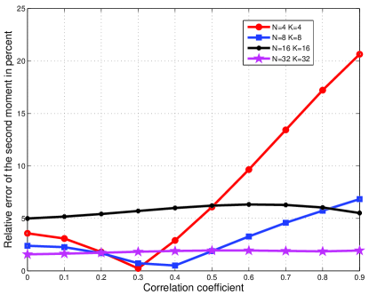
(b) Second moment of the SNR

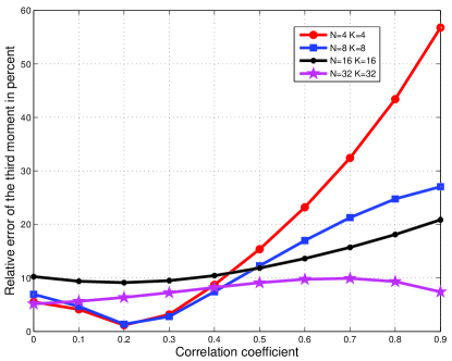
(c) Third moment of the SNR

Figure 1: Absolute value of the relative error when $N=K$

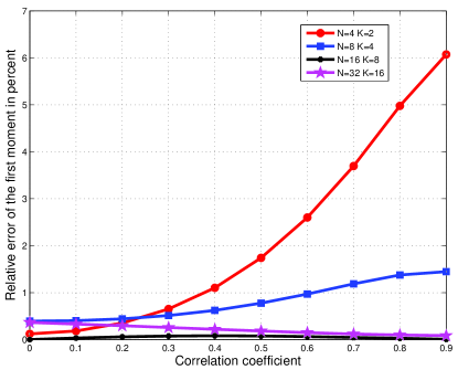
(a) First moment of the SNR

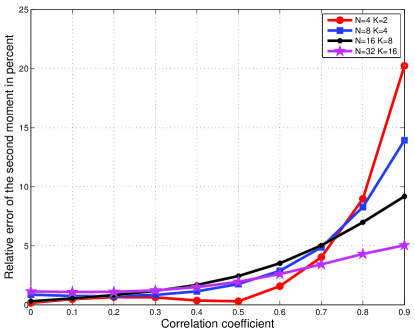
(b) Second moment of the SNR

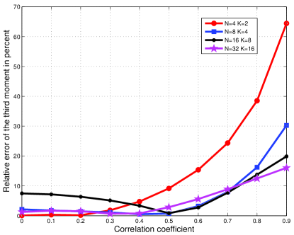
(c) Third moment of the SNR

Figure 2: Absolute value of the relative error when $N=2K$

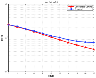
(a) $N=K=4$ and $a=0$

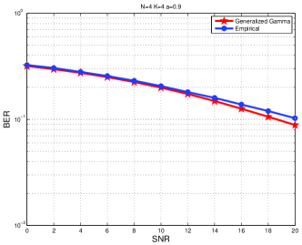
(b) $N=K=4$ and $a=0.9$

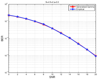
(c) $N=2K=4$ and $a=0$

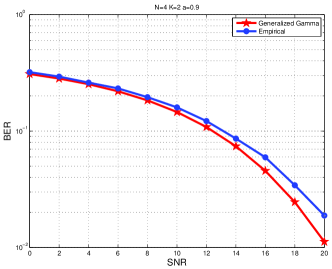
(d) $N=2K=4$ and $a=0.9$

Figure 3: BER vs input SNR

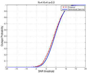
(a) $N=K=4$ and $a=0$

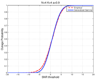
(b) $N=K=4$ and $a=0.9$

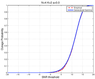
(c) $N=2K=4$ and $a=0$

(d) $N=2K=4$ and $a=0.9$

Figure 4: Outage Probability vs SNR threshold

We investigate the impact of the correlation coefficient $a$ on the accuracy of the asymptotic moments when the input SNR is set to $15$dB for $N=K$ (Fig. 1) and $N=2K$ (Fig. 2). In these figures, the relative error on the estimated first three moments $\frac{\left|\mu_{\infty}-\mu\right|}{\mu}$ ( $\mu_{\infty}$ and $\mu$ denote respectively the asymptotic and empirical moment ) is depicted with respect to the correlation coefficient $a$. These simulations show that when the number of antennas is small, the asymptotic approximation of the second and third moments degrades for large correlation coefficients ($a$ close to one). Despite these discrepancies for $a$ close to $1$, simulations show that the BER and the outage probability are well approximated even for small system dimensions. Indeed, Figure 3 shows the evolution of the empirical BER and the theoretical BER predicted by (1) versus the input SNR for different values of $a$, $K$ and $N$. In Figure 4, the saddle point approximate of the outage probability given by (2) is compared with the empirical one. In both Figures 3 and 4, $2000$ channel realizations have been considered, and in Fig. 4, the input SNR has been set to $15$ dB. These figures show that even for small system dimensions, the BER is well approximated for a wide range of SNR values. The outage probability is also well approximated except for small values of the SNR threshold that are likely to be in the tail of the asymptotic distribution.

Appendix A Proof of Theorem 1

In the sequel, we shall heavily rely on the results and techniques developed in [4]. In the sequel, ${\bf D}$ and $\widetilde{\bf D}$ are respectively $N\times N$ and $K\times K$ diagonal matrices which satisfy A1 and A2, ${\bf Z}$ is a $N\times K$ matrix whose entries are i.i.d. standard complex Gaussian, ${\bf X}$ is a $N\times K$ matrix defined by:

$${\bf X}={\bf D}^{\frac{1}{2}}{\bf Z}\widetilde{\bf D}^{\frac{1}{2}}\ .$$

We shall often write ${\bf X}=[{\bf x}_{1},\cdots,{\bf x}_{K}]$ where the ${\bf x}_{j}$’s are ${\bf X}$’s columns. We recall hereafter the mathematical tools that will be of constant use in the sequel.

A-A Notations

Define the resolvant matrix ${\bf H}$ by:

$${\bf H}=\left(\frac{t}{K}{\bf D}^{\frac{1}{2}}{\bf Z}\widetilde{\bf D}{\bf Z}^{*}{\bf D}^{\frac{1}{2}}+{\bf I}_{N}\right)^{-1}=\left(\frac{t}{K}{\bf X}{\bf X}^{*}+{\bf I}_{N}\right)^{-1}\ .$$

We introduce the following intermediate quantities:

$$\beta(t)=\frac{1}{K}\mathrm{Tr}({\bf DH}),\quad\alpha(t)=\frac{1}{K}\mathrm{Tr}({\bf D}\mathbb{E}{\bf H})\quad\textrm{and}\quad\stackrel{{\scriptstyle o}}{{\beta}}=\beta-\alpha\ .$$

Matrix $\widetilde{\bf R}(t)=\mathrm{diag}\left(\tilde{r}_{1},\cdots,\tilde{r}_{K}\right)$ is a $K\times K$ diagonal matrix defined by:

$$\widetilde{\bf R}(t)=\left({\bf I}+t\alpha(t)\widetilde{\bf D}_{K}\right)^{-1}\ .$$

Let $\tilde{\alpha}=\frac{1}{K}\mathrm{Tr}(\widetilde{\bf D}\widetilde{\bf R})$. Then, matrix ${\bf R}(t)=\mathrm{diag}\left({r}_{1},\cdots,{r}_{N}\right)$ is a $N\times N$ matrix defined by:

$${\bf R}(t)=\left({\bf I}+t\tilde{\alpha}(t){\bf D}\right)^{-1}.$$

A-B Mathematical Tools

The results below, of constant use in the proof of Theorem 1, can be found in [4].

A-B1 Differentiation formulas

$$\frac{\partial H_{pq}}{\partial{X_{ij}}} = -\frac{t}{K}\left[{\bf X}^{*}{\bf H}\right]_{jq}{H}_{pi}=-\frac{t}{K}\left[{\bf x}_{j}^{*}{\bf H}\right]_{q}H_{pi}.$$ (3)

$$\frac{\partial H_{pq}}{\partial{\overline{X_{ij}}}} = -\frac{t}{K}\left[{\bf HX}\right]_{pj}H_{iq}=-\frac{t}{K}\left[{\bf Hx}_{j}\right]_{p}H_{iq}$$ (4)

A-B2 Integration by parts formula for Gaussian functionals

: Let ${\Phi}$ be a $\mathcal{C}^{1}$ complex function polynomially bounded together with its derivatives, then:

$$\mathbb{E}\left[X_{ij}{\Phi}({\bf X})\right]=d_{i}\tilde{d}_{j}\mathbb{E}\left[\frac{\partial~{\Phi}({\bf X})}{\partial\overline{X_{ij}}}\right].$$ (5)

A-B3 Poincaré-Nash inequality

Let ${\bf X}$ and ${{\Phi}}$ be as above, then:

$$\mathrm{Var}({\Phi}({\bf X}))\leq\sum_{i=1}^{N}\sum_{j=1}^{K}d_{i}\tilde{d}_{j}\mathbb{E}\left[\left|\frac{\partial{\Phi}({\bf X})}{\partial X_{ij}}\right|^{2}+\left|\frac{\partial{\Phi}({\bf X})}{\partial\overline{X_{ij}}}\right|^{2}\right].$$ (6)

A-B4 Deterministic approximations and various estimations

Proposition 2

Let $\left({\bf A}_{K}\right)$ and $\left({\bf B}_{K}\right)$ be two sequences of respectively $N\times N$ and $K\times K$ diagonal deterministic matrices whose spectral norm are uniformly bounded in $K$, then the following hold true:

$$\frac{1}{K}\mathrm{Tr}({\bf AR})=\frac{1}{K}\mathrm{Tr}({\bf AT})+\mathcal{O}(K^{-2}),\qquad\frac{1}{K}\mathrm{Tr}({\bf B}\widetilde{\bf R})=\frac{1}{K}\mathrm{Tr}({\bf B}\widetilde{\bf T})+\mathcal{O}(K^{-2}).$$

Proposition 3

Let $\left({\bf A}_{K}\right)$, $\left({\bf B}_{K}\right)$ and $\left({\bf C}_{K}\right)$ be three sequences of $N\times N$, $K\times K$ and $N\times N$ diagonal deterministic matrices whose spectral norm are uniformly bounded in $K$. Consider the following functions:

$$\Phi({\bf X})=\frac{1}{K}\mathrm{Tr}\left({\bf AH}\frac{{\bf XBX}^{*}}{K}\right),\hskip 14.22636pt\Psi({\bf X})=\frac{1}{K}\mathrm{Tr}\left({\bf AHDH}\frac{{\bf XBX}^{*}}{K}\right).$$

Then,

1. the following estimations hold true:

   $$\mathrm{var}\,\Phi({\bf X}),\ \mathrm{var}\,\Psi({\bf X}),\ \mathrm{var}(\beta)\quad\textrm{and}\quad\mathrm{var}\left(\frac{1}{K}\mathrm{Tr}{\bf AHCH}\right)\quad\textrm{are}\quad\mathcal{O}(K^{-2})\ .$$

2. the following approximations hold true:

   $$\mathbb{E}\left[\Phi({\bf X})\right]\!\!\!\! = \!\!\!\!\frac{1}{K}\mathrm{Tr}\left(\widetilde{\bf D}\widetilde{\bf T}{\bf B}\right)\frac{1}{K}\mathrm{Tr}\left({\bf ADT}\right)+\mathcal{O}(K^{-2}),$$ (7)

   $$\mathbb{E}\left[\Psi({\bf X})\right]\!\!\!\! = \!\!\!\!\frac{1}{1-t^{2}\gamma\tilde{\gamma}}\left(\frac{1}{K^{2}}\mathrm{Tr}\left(\widetilde{\bf D}\widetilde{\bf T}{\bf B}\right)\mathrm{Tr}({\bf AD}^{2}{\bf T}^{2})-\frac{t\gamma}{K^{2}}\mathrm{Tr}\left(\widetilde{\bf D}^{2}\widetilde{\bf T}^{2}{\bf B}\right)\mathrm{Tr}({\bf ADT})\right)+\mathcal{O}(K^{-2}),\ \ \ \ \$$ (8)

   $$\mathbb{E}\frac{1}{K}\mathrm{Tr}\left[{\bf AHDH}\right]\!\!\!\! = \!\!\!\!\frac{1}{1-t^{2}\gamma\tilde{\gamma}}\frac{1}{K}\mathrm{Tr}({\bf AD}{\bf T}^{2})+\mathcal{O}(K^{-2}).$$ (9)

Proofs of Propositions 2 and 3 are essentially provided in [4]. In the same vein, the following proposition will be needed.

Proposition 4

Let $\left({\bf A}_{K}\right)$, $\left({\bf B}_{K}\right)$ and $\left({\bf C}_{K}\right)$ be three sequences of $N\times N$, $K\times K$ and $N\times N$ diagonal deterministic matrices whose spectral norm are uniformly bounded in $K$. Consider the following function:

$$\varphi({\bf X})=\frac{1}{K}\mathrm{Tr}\left[{\bf CHAHAH}\frac{{\bf XBX}^{*}}{K}\right]\ .$$

Then $\mathrm{var}\,\varphi({\bf X})=\mathcal{O}(K^{-2})$ and $\mathrm{var}\left(\frac{1}{K}\mathrm{Tr}{\bf AHAHAH}\right)=\mathcal{O}(K^{-2})\ .$

Proof of Proposition 4 is essentially the same as the proof of Proposition 3-1). It is provided for completeness and postponed to appendix B.

A-C End of proof of Theorem 1

We are now in position to complete the proof of Theorem 1. Using the notations of [4], the SNR writes:

$$\beta_{K}=\frac{tp_{0}}{K}{\bf z}^{*}{\bf D}^{\frac{1}{2}}{\bf H(t)}{\bf D}^{\frac{1}{2}}{\bf z},$$

where $t=\frac{1}{\rho}$. Hence, the third moment is given by:

$$\mathbb{E}\left(\beta_{K}-\mathbb{E}\beta_{K}\right)^{3} = \frac{(tp_{0})^{3}}{K^{3}}\mathbb{E}\left({\bf z}^{*}{\bf D}^{\frac{1}{2}}{\bf H}{\bf D}^{\frac{1}{2}}{\bf z}-\mathbb{E}\mathrm{Tr}{\bf DH}\right)^{3},$$ (10)

$$= \frac{(tp_{0})^{3}}{K^{3}}\mathbb{E}\left({\bf z}^{*}{\bf D}^{\frac{1}{2}}{\bf H}{\bf D}^{\frac{1}{2}}{\bf z}-\mathrm{Tr}{\bf DH}+\mathrm{Tr}{\bf DH}-\mathbb{E}\mathrm{Tr}{\bf DH}\right)^{3},$$

$$= \frac{(tp_{0})^{3}}{K^{3}}\left[\mathbb{E}\left({\bf z}^{*}{\bf D}^{\frac{1}{2}}{\bf H}{\bf D}^{\frac{1}{2}}{\bf z}-\mathrm{Tr}{\bf DH}\right)^{3}+3\mathbb{E}\left({\bf z}^{*}{\bf D}^{\frac{1}{2}}{\bf H}{\bf D}^{\frac{1}{2}}{\bf z}-\mathrm{Tr}{\bf DH}\right)^{2}\left(\mathrm{Tr}{\bf DH}-\mathbb{E}\mathrm{Tr}{\bf DH}\right)\right.$$

$$\left.+3\mathbb{E}\left({\bf z}^{*}{\bf D}^{\frac{1}{2}}{\bf H}{\bf D}^{\frac{1}{2}}{\bf z}-\mathrm{Tr}{\bf DH}\right)\left(\mathrm{Tr}{\bf DH}-\mathbb{E}\mathrm{Tr}{\bf DH}\right)^{2}+\mathbb{E}\left(\mathrm{Tr}{\bf DH}-\mathbb{E}\mathrm{Tr}{\bf DH}\right)^{3}\right],$$

$$= \frac{(tp_{0})^{3}}{K^{3}}\left[\mathbb{E}\left({\bf z}^{*}{\bf D}^{\frac{1}{2}}{\bf H}{\bf D}^{\frac{1}{2}}{\bf z}-\mathrm{Tr}{\bf DH}\right)^{3}+3\mathbb{E}\left({\bf z}^{*}{\bf D}^{\frac{1}{2}}{\bf H}{\bf D}^{\frac{1}{2}}{\bf z}-\mathrm{Tr}{\bf DH}\right)^{2}\left(\mathrm{Tr}{\bf DH}-\mathbb{E}\mathrm{Tr}{\bf DH}\right)\right.$$

$$\left.+\mathbb{E}\left(\mathrm{Tr}{\bf DH}-\mathbb{E}\mathrm{Tr}{\bf DH}\right)^{3}\right]$$

In order to deal with the first term of the right-hand side of (10), notice that if ${\bf M}$ is a deterministic matrix and ${\bf x}$ is a standard Gaussian vector, then:

$$\mathbb{E}\left({\bf x}^{*}{\bf M}{\bf x}-\mathrm{Tr}{\bf M}\right)^{3}=\mathrm{Tr}({\bf M}^{3})\mathbb{E}\left(|x_{1}|^{2}-1\right)^{3}$$

(such an identity can be easily proved by considering the spectral decomposition of ${\bf M}$). Hence,

$$\mathbb{E}\left({\bf z}^{*}{\bf D}^{\frac{1}{2}}{\bf H}{\bf D}^{\frac{1}{2}}{\bf z}-\mathrm{Tr}{\bf DH}\right)^{3} = \mathbb{E}\mathrm{Tr}\left({\bf DH}\right)^{3}\mathbb{E}\left(|Z_{11}|^{2}-1\right)^{3},$$

$$= 2\mathbb{E}\mathrm{Tr}\left({\bf DHDHDH}\right).$$

The second term of the right-hand side of (10) is uniformly bounded in $K$. Indeed:

$$3\mathbb{E}\left({\bf z}^{*}{\bf D}^{\frac{1}{2}}{\bf H}{\bf D}^{\frac{1}{2}}{\bf z}-\mathrm{Tr}({\bf DH})\right)^{2} = 3\mathbb{E}\left(|Z_{11}|^{2}-1\right)^{2}\mathrm{Tr}{\bf DHDH}\left(\mathrm{Tr}{\bf DH}-\mathbb{E}\mathrm{Tr}{\bf DH}\right),$$

$$\leq 3\sqrt{\mathrm{var}\left(\mathrm{Tr}{\bf DHDH}\right)}\sqrt{\mathrm{var}\left(\mathrm{Tr}{\bf DH}\right)}$$

which is ${\mathcal{O}}(1)$ according to Proposition 3. It remains to deal with $\mathbb{E}\left(\mathrm{Tr}{\bf DH}-\mathbb{E}\mathrm{Tr}{\bf DH}\right)^{3}$, which can be proved to be uniformly bounded in $K$ using concentration results for the spectral measure of random matrices [21] (see also [15, eq.(86)-(87)], where details are provided). Consequently, we end up with the following approximation:

$$K^{2}\mathbb{E}\left(\beta_{K}-\mathbb{E}\beta_{K}\right)^{3}=\frac{(tp_{0})^{3}}{K}\mathbb{E}\left(|Z_{11}|^{2}-1\right)^{3}\mathbb{E}\mathrm{Tr}{\bf DHDHDH}+\mathcal{O}\left(K^{-1}\right)$$

which is deterministic but still depends on the distribution of the entries via the expectation operator $\mathbb{E}$. The rest of the proof is devoted to provide a deterministic approximation of $\mathbb{E}\mathrm{Tr}\left({\bf DHDHDH}\right)$ depending on $\gamma$, $\tilde{\gamma}$, ${\bf T}$ and $\widetilde{\bf T}$.

Note that ${\bf H}={\bf I}-\frac{t}{K}{\^{A}~\bf HXX}^{*}$, thus:

$$\left[{\bf HDHDH}\right]_{pp} = \left[{\bf HDHD}\right]_{pp}-t\left[{\bf HDHDH}\frac{\bf XX^{*}}{K}\right]_{pp},$$ (11)

$$= \left[{\bf HDHD}\right]_{pp}-\frac{t}{K}\sum_{j=1}^{K}\left[{\bf HDHDHx}_{j}\right]_{p}\overline{{X}_{pj}}.$$

Let us deal with the second term of (11). We have:

$$\mathbb{E}\frac{1}{K}\left[{\bf HDHDHx}_{j}\right]_{p}\overline{{X}_{pj}}=\frac{1}{K}\sum_{k=1}^{N}\mathbb{E}\left(\left[{\bf HDHDH}\right]_{pk}X_{kj}\overline{X_{pj}}\right).$$

Using the integration by part formula (5), we get:

$$\mathbb{E}\left[{\bf HDHDHx}_{j}\right]_{p}\overline{{X}_{pj}} = \sum_{k=1}^{N}d_{k}\tilde{d}_{j}\delta(p-k)\mathbb{E}\left[{\bf HDHDH}\right]_{pk}+\sum_{k=1}^{N}d_{k}\tilde{d}_{j}\mathbb{E}\left[\overline{X_{pj}}\sum_{\ell,m=1}^{N}\frac{\partial\left[H_{p\ell}d_{\ell}d_{m}H_{\ell m}H_{mk}\right]}{\partial{\overline{X_{kj}}}}\right],$$

$$= d_{p}\tilde{d}_{j}\mathbb{E}\left[{\bf HDHDH}\right]_{pp}-\frac{t}{K}\sum_{k,\ell,m=1}^{N}d_{k}\tilde{d}_{j}d_{m}d_{\ell}\mathbb{E}\left[\overline{X_{pj}}\left[{\bf Hx}_{j}\right]_{p}H_{k\ell}H_{\ell m}H_{mk}\right]$$

$$-\frac{t}{K}\sum_{k,\ell,m=1}^{N}d_{k}\tilde{d}_{j}d_{m}d_{\ell}\mathbb{E}\left[\overline{X_{pj}}H_{p\ell}\left[{\bf Hx}_{j}\right]_{\ell}H_{km}H_{mk}\right]$$

$$-\frac{t}{K}\sum_{k,\ell,m=1}^{N}d_{k}\tilde{d}_{j}d_{m}d_{\ell}\mathbb{E}\left[H_{p\ell}H_{\ell m}\left[{\bf Hx}_{j}\right]_{m}H_{kk}\right].$$

$$= d_{p}\tilde{d}_{j}\mathbb{E}\left[{\bf HDHDH}\right]_{pp}-\frac{t}{K}\tilde{d}_{j}\mathbb{E}\left[\left[{\bf Hx}_{j}\right]_{p}\overline{X_{pj}}\mathrm{Tr}\left({\bf DHDHDH}\right)\right]$$

$$-\frac{t}{K}\tilde{d}_{j}\mathbb{E}\left[\left[{\bf HDHx}_{j}\right]_{p}\overline{X_{pj}}\mathrm{Tr}\left({\bf DHDH}\right)\right]-\frac{t}{K}\tilde{d}_{j}\mathbb{E}\left[\left[{\bf HDHDHx}_{j}\right]_{p}\overline{X_{pj}}\mathrm{Tr}\left({\bf DH}\right)\right].$$

Substituting in the last term $\frac{1}{K}\mathrm{Tr}{\bf DH}=\stackrel{{\scriptstyle o}}{{\beta}}+\alpha$ where $\stackrel{{\scriptstyle o}}{{\beta}}=\beta-\alpha$, we get:

$$\mathbb{E}\left[{\bf HDHDHx}_{j}\right]_{p}\overline{{X}_{pj}} = d_{p}\tilde{d}_{j}\mathbb{E}\left[{\bf HDHDH}\right]_{pp}-\frac{t}{K}\tilde{d}_{j}\mathbb{E}\left[\left[{\bf Hx}_{j}\right]_{p}\overline{X_{pj}}\mathrm{Tr}\left({\bf DHDHDH}\right)\right]$$

$$-\frac{t}{K}\tilde{d}_{j}\mathbb{E}\left[\left[{\bf HDHx}_{j}\right]_{p}\overline{X_{pj}}\mathrm{Tr}\left({\bf DHDH}\right)\right]-t\tilde{d}_{j}\mathbb{E}\left[\left[{\bf HDHDHx}_{j}\right]_{p}\overline{X_{pj}}\stackrel{{\scriptstyle o}}{{\beta}}\right]$$

$$-t\tilde{d}_{j}\mathbb{E}\left[\left[{\bf HDHDHx}_{j}\right]_{p}\overline{X_{pj}}\right]\alpha.$$

Therefore, we have:

$$\left(1+t\alpha\tilde{d}_{j}\right)\mathbb{E}\left[\left[{\bf HDHDHx}_{j}\right]_{p}\overline{X_{pj}}\right] = d_{p}\tilde{d}_{j}\mathbb{E}\left[{\bf HDHDH}\right]_{pp}-\frac{t}{K}\mathbb{E}\left[\left[{\bf Hx}_{j}\right]_{p}\overline{X_{pj}}\tilde{d}_{j}\mathrm{Tr}\left[{\bf DHDHDH}\right]\right]$$

$$-\frac{t}{K}\tilde{d}_{j}\mathbb{E}\left[\left[{\bf HDHx}_{j}\right]_{p}\overline{X_{pj}}\mathrm{Tr}\left[{\bf DHDH}\right]\right]-t\tilde{d}_{j}\mathbb{E}\left[\left[{\bf HDHDHx}_{j}\right]_{p}\overline{X_{pj}}\stackrel{{\scriptstyle o}}{{\beta}}\right].$$

Multiplying the right hand and the left hand sides by $\tilde{r}_{j}=\frac{1}{1+t\alpha\tilde{d}_{j}}$, we get:

$$\mathbb{E}\left[{\bf HDHDHx}_{j}\right]_{p}\overline{X_{pj}}\quad=\quad\tilde{r}_{j}d_{p}\tilde{d}_{j}\mathbb{E}\left[{\bf HDHDH}\right]_{pp}-\frac{t}{K}\tilde{r}_{j}\mathbb{E}\left[\left[{\bf Hx}_{j}\right]_{p}\overline{X_{pj}}\tilde{d}_{j}\mathrm{Tr}\left[{\bf DHDHDH}\right]\right]\\ -\frac{t}{K}\tilde{d}_{j}\tilde{r}_{j}\mathbb{E}\left[\left[{\bf HDHx}_{j}\right]_{p}\overline{X_{pj}}\mathrm{Tr}\left[{\bf DHDH}\right]\right]-t\tilde{d}_{j}\tilde{r}_{j}\mathbb{E}\left[\left[{\bf HDHDHx}_{j}\right]_{p}\overline{X_{pj}}\stackrel{{\scriptstyle o}}{{\beta}}\right].$$ (12)

Plugging (12) into (11), we obtain:

$$\mathbb{E}\left[{\bf HDHDH}\right]_{pp} = \mathbb{E}\left[{\bf HDHD}\right]_{pp}-\sum_{j=1}^{K}\frac{t}{K}\tilde{r}_{j}d_{p}\tilde{d}_{j}\mathbb{E}\left[{\bf HDHDH}\right]_{pp}+\frac{t^{2}}{K^{2}}\sum_{j=1}^{K}\tilde{r}_{j}\mathbb{E}\left[{\bf Hx}_{j}\right]_{p}\overline{X_{pj}}\tilde{d}_{j}\mathrm{Tr}\left[{\bf DHDHDH}\right]$$

$$+\frac{t^{2}}{K^{2}}\sum_{j=1}^{K}\tilde{d}_{j}\tilde{r}_{j}\mathbb{E}\left[{\bf HDHx}_{j}\right]_{p}\overline{X_{p,j}}\mathrm{Tr}\left[{\bf DHDH}\right]+\frac{t}{K}\sum_{j=1}^{K}\tilde{d}_{j}\tilde{r}_{j}\mathbb{E}\left[{\bf HDHDHx}_{j}\right]_{p}\overline{X_{p,j}}\stackrel{{\scriptstyle o}}{{\beta}},$$

$$= \mathbb{E}\left[{\bf HDHD}\right]_{pp}-t\tilde{\alpha}d_{p}\mathbb{E}\left[{\bf HDHDH}\right]_{pp}+\frac{t^{2}}{K^{2}}\mathbb{E}\mathrm{Tr}({\bf DHDHDH})\left[{\bf HX\widetilde{\bf R}\widetilde{\bf D}{\bf X^{*}}}\right]_{pp}$$

$$+\frac{t^{2}}{K^{2}}\mathbb{E}\mathrm{Tr}\left[{\bf DHDH}\right]\left[{\bf HDHX}\widetilde{\bf D}{\widetilde{\bf R}{\bf X^{*}}}\right]_{pp}+\frac{t^{2}}{K}\mathbb{E}\stackrel{{\scriptstyle o}}{{\beta}}\left[{\bf HDHDHX\widetilde{\bf D}\widetilde{\bf R}{X}^{*}}\right]_{pp}.$$

Hence,

$$(1+t\tilde{\alpha}d_{p})\mathbb{E}\left[{\bf HDHDH}\right]_{pp} = \mathbb{E}\left[{\bf HDHD}\right]_{pp}+\frac{t^{2}}{K^{2}}\mathbb{E}\mathrm{Tr}\left[{\bf DHDHDH}\right]\left[{\bf HX}\widetilde{\bf R}\widetilde{\bf D}{\bf X}^{*}\right]_{pp}$$

$$+\frac{t^{2}}{K^{2}}\mathbb{E}\mathrm{Tr}\left[{\bf DHDH}\right]\left[{\bf HDHX}\widetilde{\bf D}\widetilde{\bf R}{\bf X^{*}}\right]_{pp}+\frac{t^{2}}{K}\mathbb{E}\stackrel{{\scriptstyle o}}{{\beta}}\left[{\bf HDHDHX\widetilde{D}\widetilde{R}X}^{*}\right]_{pp}\ .$$

Multiplying the left and right hand sides by $r_{p}=\frac{1}{1+t\tilde{\alpha}d_{p}}$, we get:

$$\mathbb{E}\left[{\bf HDHDH}\right]_{pp} = r_{p}\mathbb{E}\left[{\bf HDHD}\right]_{pp}+\frac{t^{2}}{K^{2}}r_{p}\mathbb{E}\mathrm{Tr}\left[{\bf DHDHDH}\right]\left[{\bf HX}\widetilde{\bf R}\widetilde{\bf D}{\bf X}^{*}\right]_{pp}$$ (13)

$$+\frac{t^{2}}{K^{2}}r_{p}\mathbb{E}\mathrm{Tr}\left[{\bf DHDH}\right]\left[{\bf HDHX}\widetilde{\bf D}\widetilde{\bf R}{\bf X}^{*}\right]_{pp}+\frac{t^{2}}{K}r_{p}\mathbb{E}\stackrel{{\scriptstyle o}}{{\beta}}\left[{\bf HDHDHX}\widetilde{\bf D}\widetilde{\bf R}{\bf X}^{*}\right]_{pp}.$$

Multiplying by $d_{p}$, summing over $p$ and dividing by $K$, we obtain:

$$\mathbb{E}\frac{1}{K}\mathrm{Tr}\left[{\bf DHDHDH}\right] = \mathbb{E}\frac{1}{K}\sum_{p=1}^{K}d_{p}\left[{\bf HDHDH}\right]_{pp},$$ (14)

$$= \frac{1}{K}\sum_{p=1}^{K}r_{p}d_{p}\mathbb{E}\left[{\bf HDHD}\right]_{pp}+\frac{t^{2}}{K^{3}}\mathbb{E}\,\mathrm{Tr}\left({\bf DHDHDH}\right)\mathrm{Tr}\left({\bf DRH}{\bf X\widetilde{\bf R}\widetilde{\bf D}{\bf X}^{*}}\right)$$

$$+\frac{t^{2}}{K^{3}}\mathbb{E}\mathrm{Tr}\left({\bf DHDH}\right)\mathrm{Tr}\left({\bf DRHDHX}\widetilde{\bf D}\widetilde{\bf R}{\bf X}^{*}\right)$$

$$+\frac{t^{2}}{K^{2}}\mathbb{E}\ \stackrel{{\scriptstyle o}}{{\beta}}\mathrm{Tr}\left({\bf DRHDHDH}{\bf X\widetilde{D}\widetilde{R}X^{*}}\right),$$

$$\stackrel{{\scriptstyle\triangle}}{{=}} \chi_{1}+\chi_{2}+\chi_{3}+\chi_{4},$$

where:

$$\chi_{1} = \frac{1}{K}\mathbb{E}\mathrm{Tr}\left({\bf DRHDHD}\right)\ ,$$

$$\chi_{2} = \frac{t^{2}}{K}\mathbb{E}\mathrm{Tr}\left({\bf DHDHDH}\right)\frac{1}{K}\mathrm{Tr}\left({\bf DRH}\frac{\bf X\widetilde{D}\widetilde{R}X^{*}}{K}\right)\ ,$$

$$\chi_{3} = \frac{t^{2}}{K}\mathbb{E}\mathrm{Tr}\left({\bf DHDH}\right)\frac{1}{K}\mathrm{Tr}\left({\bf DRHDH}\frac{\bf X\widetilde{D}\widetilde{R}X^{*}}{K}\right)\ ,$$

$$\chi_{4} = \frac{t^{2}}{K}\mathbb{E}\,\stackrel{{\scriptstyle o}}{{\beta}}\mathrm{Tr}\left({\bf DRHDHDH}\frac{\bf X\widetilde{D}\widetilde{R}X^{*}}{K}\right)\ .$$

According to Proposition 3, $\mathrm{var}\frac{1}{K}\mathrm{Tr}\left({\bf DRHDHDH}\frac{{\bf X\widetilde{\bf D}\widetilde{\bf R}\bf X}^{*}}{K}\right)$ is of order $\mathcal{O}(K^{-2})$. Similarly, $\mathrm{var}({\beta})=\mathcal{O}(K^{-2})$. Hence, using Cauchy-Schwartz inequality, we get the estimation $\chi_{4}=\mathcal{O}(K^{-2})$. It remains to work out the expressions involved in $\chi_{1}$, $\chi_{2}$ and $\chi_{3}$ by removing the terms with expectation and replacing them with deterministic equivalents.

Since $\mathrm{var}\frac{1}{K}\mathrm{Tr}\left({\bf DRH}\frac{{\bf X\widetilde{\bf D}\widetilde{\bf R}{\bf X}}^{*}}{K}\right)=\mathcal{O}(K^{-2})$ by Proposition 3 and $\mathrm{var}(\frac{1}{K}\mathrm{Tr}{\bf DHDHDH})=\mathcal{O}(K^{-2})$ by Proposition 4, we have:

$$\chi_{2} = \frac{t^{2}}{K}\mathbb{E}\mathrm{Tr}\left({\bf DHDHDH}\right)\mathbb{E}\left(\frac{1}{K}\mathrm{Tr}\left[{\bf DRH}\frac{\bf X\widetilde{\bf D}{\widetilde{R}}{\bf X}^{*}}{K}\right]\right)+\mathcal{O}(K^{-2}),$$ (15)

$$\stackrel{{\scriptstyle(a)}}{{=}} \frac{t^{2}}{K}\mathbb{E}\mathrm{Tr}\left({\bf DHDHDH}\right)\frac{1}{K}\mathrm{Tr}\left(\widetilde{\bf D}\widetilde{\bf T}\widetilde{\bf D}\widetilde{\bf R}\right)\frac{1}{K}\mathrm{Tr}\left({\bf DRDT}\right)+\mathcal{O}(K^{-2}),$$

$$\stackrel{{\scriptstyle(b)}}{{=}} \frac{t^{2}}{K}\mathbb{E}\mathrm{Tr}\left({\bf DHDHDH}\right)\gamma\tilde{\gamma}+\mathcal{O}(K^{-2})\ .$$

where (a) follows from Proposition 3-2) and (b), from Proposition 2. Similar arguments yield:

$$\chi_{3} = \frac{t^{2}}{K}\mathbb{E}\mathrm{Tr}\left({\bf DHDH}\right)\mathbb{E}\left(\frac{1}{K}\mathrm{Tr}\left[{\bf DRHDH\frac{{\bf X\widetilde{\bf D}\widetilde{\bf R}{\bf X}^{*}}}{K}}\right]\right)+\mathcal{O}(K^{-2}),$$ (16)

$$= \frac{t^{2}\gamma}{(1-t^{2}\gamma\tilde{\gamma})^{2}}\left[\frac{1}{K}\mathrm{Tr}\left(\widetilde{\bf D}\widetilde{\bf T}\widetilde{\bf D}\widetilde{\bf R}\right)\frac{1}{K}\mathrm{Tr}\left({\bf DR}{\bf D}^{2}{\bf T}^{2}\right)-\frac{t\gamma}{K}\mathrm{Tr}\left(\widetilde{\bf D}^{2}\widetilde{\bf T}^{2}\widetilde{\bf D}\widetilde{\bf R}\right)\frac{1}{K}\mathrm{Tr}({\bf DRDT})\right]+\mathcal{O}(K^{-2})\ ,$$

$$= \frac{t^{2}\gamma}{(1-t^{2}\gamma\tilde{\gamma})^{2}}\left[\frac{\tilde{\gamma}}{K}\mathrm{Tr}({\bf D}^{3}{\bf T}^{3})-\frac{t\gamma^{2}}{K}\mathrm{Tr}(\widetilde{\bf D}^{3}\widetilde{\bf T}^{3})\right]+\mathcal{O}(K^{-2})$$

and

$$\chi_{1} = \frac{1}{1-t^{2}\gamma\tilde{\gamma}}\frac{1}{K}\mathrm{Tr}\left({\bf D}^{2}{\bf R}{\bf DT}^{2}\right)+\mathcal{O}(K^{-2})$$ (17)

$$= \frac{1}{1-t^{2}\gamma\tilde{\gamma}}\frac{1}{K}\mathrm{Tr}({\bf D}^{3}{\bf T}^{3})+\mathcal{O}(K^{-2}).$$

Plugging (16), (15) and (17) into (14), we obtain:

$$\frac{1}{K}\mathbb{E}\mathrm{Tr}({\bf DHDHDH})=\frac{1}{K(1-t^{2}\gamma\tilde{\gamma})^{3}}\mathrm{Tr}{\bf D}^{3}{\bf T}^{3}-\frac{t^{3}\gamma^{3}}{K(1-t^{2}\gamma\tilde{\gamma})^{3}}\mathrm{Tr}\widetilde{\bf T}^{3}\widetilde{\bf D}^{3}+\mathcal{O}(K^{-2}).\\$$

Hence,

$$K^{2}\mathbb{E}\left(\frac{\beta_{K}}{p_{0}}-\mathbb{E}\frac{\beta_{K}}{p_{0}}\right)^{3} = \frac{\rho^{3}}{K\left(\rho^{2}-\gamma\tilde{\gamma}\right)^{3}}\left[\mathrm{Tr}{\bf D}^{3}{\bf T}^{3}-\frac{\gamma^{3}}{\rho^{3}}\mathrm{Tr}\widetilde{\bf D}^{3}\widetilde{\bf T}^{3}\right]\mathbb{E}\left(\left|Z_{11}\right|^{2}-1\right)^{3}+\mathcal{O}\left(\frac{1}{K}\right),$$

$$= \frac{2\rho^{3}}{K\left(\rho^{2}-\gamma\tilde{\gamma}\right)^{3}}\left[\mathrm{Tr}{\bf D}^{3}{\bf T}^{3}-\frac{\gamma^{3}}{\rho^{3}}\mathrm{Tr}\widetilde{\bf D}^{3}\widetilde{\bf T}^{3}\right]+\mathcal{O}\left(\frac{1}{K}\right).$$

The fact that $\nu_{K}=\frac{2\rho^{3}}{K\left(\rho^{2}-\gamma\tilde{\gamma}\right)^{3}}\left[\mathrm{Tr}{\bf D}^{3}{\bf T}^{3}-\frac{\gamma^{3}}{\rho^{3}}\mathrm{Tr}\widetilde{\bf D}^{3}\widetilde{\bf T}^{3}\right]$ is of order ${\mathcal{O}}(1)$ is straightforward and its proof is omitted. Proof of Theorem 1 is completed.

Appendix B Proof of Proposition 4

The proof mainly relies on Poincaré-Nash inequality. Using the Poincaré-Nash inequality, we have:

$$\mathrm{var}(\varphi({\bf X}))\leq\sum_{i=1}^{N}\sum_{j=1}^{K}d_{i}\tilde{d}_{j}\mathbb{E}\left|\frac{\partial\varphi}{\partial X_{ij}}\right|^{2}+\sum_{i=1}^{N}\sum_{j=1}^{K}d_{i}\tilde{d}_{j}\mathbb{E}\left|\frac{\partial\varphi}{\partial\overline{X_{ij}}}\right|^{2}\\ .$$

We only deal with the first term of the last inequality (the second term can be handled similarly). We have $\varphi({\bf X})=\frac{1}{K^{2}}\sum_{p,r,s,t=1}^{N}\sum_{u=1}^{K}c_{pp}H_{pr}A_{rr}H_{rs}A_{ss}H_{st}X_{tu}B_{uu}X^{*}_{pu}$. After straightforward calculations using the differentiation formula (3), we get that:

$$\frac{\partial\varphi}{\partial X_{ij}}=\phi_{ij}^{(1)}+\phi_{ij}^{(2)}+\phi_{ij}^{(3)}+\phi_{ij}^{(4)},$$

where:

$$\phi_{ij}^{(1)} = -\frac{t}{K^{3}}\left[{\bf X}^{*}{\bf HAHAHXBX}^{*}{\bf CH}\right]_{ji},\quad\phi_{ij}^{(2)}\quad=\quad-\frac{t}{K^{3}}\left[{\bf X}^{*}{\bf HAHXBX}^{*}{\bf CHAH}\right]_{ji},$$

$$\phi_{ij}^{(3)} = -\frac{t}{K^{3}}\left[{\bf X}^{*}{\bf HXBX}^{*}{\bf CHAHAH}\right]_{ji},\quad\phi_{ij}^{(4)}\quad=\quad\frac{1}{K^{2}}\left[{\bf BX}^{*}{\bf CHAHAH}\right]_{ji}.$$

Hence, $\left|\frac{\partial\varphi}{\partial X_{ij}}\right|^{2}\leq 4\left(\left|\phi_{ij}^{(1)}\right|^{2}+\left|\phi_{ij}^{(2)}\right|^{2}+\left|\phi_{ij}^{(3)}\right|^{2}+\left|\phi_{ij}^{(4)}\right|^{2}\right)$ and

$$\sum_{i=1}^{N}\sum_{j=1}^{K}d_{i}\tilde{d}_{j}\mathbb{E}\left[\left|\frac{\partial\varphi}{\partial X_{ij}}\right|^{2}\right] \leq \frac{4t^{2}}{K^{6}}\mathbb{E}\mathrm{Tr}\left({\bf DHCXBX}^{*}{\bf HAHAH}{\bf X}\widetilde{\bf D}{\bf X}^{*}{\bf HAHAH}{\bf XBX}^{*}{\bf CH}\right)$$

$$+\frac{4t^{2}}{K^{6}}\mathbb{E}\mathrm{Tr}\left({\bf DHAHCXBX}^{*}{\bf HAHX}\widetilde{\bf D}{\bf X}^{*}{\bf HAHXBX}^{*}{\bf CHAH}\right)$$

$$+\frac{4t^{2}}{K^{6}}\mathbb{E}\mathrm{Tr}\left({\bf DHAHAHCXBX}^{*}{\bf HX}\widetilde{\bf D}{\bf X}^{*}{\bf HXBX}^{*}{\bf CHAHAH}\right)$$

$$+\frac{4}{K^{4}}\mathbb{E}\mathrm{Tr}\left({\bf DHAHAHCXB}\widetilde{\bf D}{\bf B}{\bf X}^{*}{\bf CHAHAH}\right).$$

We only prove that the first term of the right hand side is of order $K^{-2}$; the other terms being handled similarly. Using Cauchy-Schwartz inequality, we get:

$$4\sum_{i=1}^{N}\sum_{j=1}^{K}d_{i}\tilde{d}_{j}\mathbb{E}\left|\phi_{ij}^{1}\right|^{2} \leq \frac{4t^{2}d_{\mathrm{max}}\|{\bf H}\|^{2}\|{\bf C}\|^{2}}{K^{6}}\mathbb{E}\mathrm{Tr}\left(\left({\bf HA}\right)^{2}{\bf H}{\bf X}\widetilde{\bf D}{\bf X}^{*}{\bf H}\left({\bf AH}\right)^{2}\left({\bf XBX}^{*}\right)^{2}\right),$$

$$\leq \frac{4t^{2}}{K^{6}}d_{\mathrm{max}}\|{\bf H}\|^{2}\|{\bf C}\|^{2}\left(\mathbb{E}\mathrm{Tr}\left({\bf HA}\right)^{2}{\bf H}{\bf X}\widetilde{\bf D}{\bf X}^{*}{\bf H}\left({\bf AH}\right)^{2}\left({\bf HA}\right)^{2}{\bf H}{\bf X}\widetilde{\bf D}{\bf X}^{*}{\bf H}\left({\bf AH}\right)^{2}\right)^{\frac{1}{2}}$$

$$\times \left(\mathbb{E}\mathrm{Tr}\left({\bf XBX}^{*}\right)^{4}\right)^{\frac{1}{2}}$$

$$\leq \frac{4t^{2}}{K^{2}}d_{\mathrm{max}}\|{\bf H}\|^{8}\|{\bf C}\|^{2}\|{\bf A}\|^{4}\sqrt{\mathbb{E}\frac{1}{K}\left(\frac{{\bf X}\widetilde{\bf D}{\bf X}^{*}}{K}\right)^{2}}\sqrt{\mathbb{E}\frac{1}{K}\left(\frac{{\bf X}{\bf B}{\bf X}^{*}}{K}\right)^{4}},$$

where the first inequality follows by using the fact that $\left|\mathrm{Tr}{\bf AB}\right|\leq\|{\bf B}\|\mathrm{Tr}\left({\bf A}\right)$, ${\bf A}$ being hermitian non-negative matrix and the second follows by applyig twice Cauchy-Schwartz inequalities: $\mathrm{Tr}\left({\bf AB}\right)\leq\sqrt{\mathrm{Tr}\left({\bf AA}^{*}\right)}\sqrt{\mathrm{Tr}\left({\bf BB}^{*}\right)}$ and $\mathbb{E}{XY}\leq\sqrt{\mathbb{E}X^{2}}\sqrt{\mathbb{E}Y^{2}}$. We end up the proof of the first statement by using the fact that $\frac{1}{K}\mathbb{E}\left[\frac{1}{K}\mathrm{Tr}\left(\frac{1}{K}{\bf X}{\bf B}_{K}{\bf X}^{*}\right)^{n}\right]$ is uniformly bounded in $K$ whenever ${\bf B}_{K}$ is a sequence of diagonal matrices with uniformly bounded spectral norm and $n$ is a given integer.

The second statement follows from the resolvent identity:

$$\frac{1}{K}\mathrm{Tr}{\bf AHAHAH}=\frac{1}{K}\mathrm{Tr}{\bf AHAHA}-\frac{t}{K}\mathrm{Tr}{\bf AHAHAH{\bf XX}^{*}}.$$

According to the first part of the proposition,

$$\mathrm{var}\left(\frac{1}{K}\mathrm{Tr}{\bf AHAHAH{\bf XX}^{*}}\right)=\mathcal{O}(K^{-2})\ .$$

Now, $\mathrm{Tr}{\bf AHAHA}=\mathrm{Tr}{\bf A^{2}HAH}$ and $\mathrm{var}\frac{1}{K}\mathrm{Tr}{\bf A^{2}HAH}=\mathcal{O}(K^{-2})$ by Proposition 3-1). Hence, applying inequality $\mathrm{var}(X+Y)\leq\mathrm{var}(X)+\mathrm{var}(Y)+2\sqrt{\mathrm{var}(X)\mathrm{var}(Y)}$ yields the desired result. Proof of Proposition 4 is completed.

(a) First moment of the SNR

References

• [1] I. E. Telatar, “Capacity of Multi-antenna Gaussian Channels,” European Transactions on Telecommunications and Related Technologies, vol. 10, no. 6, pp. 585–596, November 1999.
• [2] B.M. Hochwald, T.L. Marzetta, and V. Tarokh, “Multiple-Antenna Channel Hardening and Its Implications for Rate Feedback and Scheduling,” IEEE Transactions on Information Theory, vol. 50, no. 9, pp. 1893–1909, September 2004.
• [3] R. Narasimhan, “Transmit Antenna Selection Based on Outage Probability for Correlated MIMO Multiple Access Channels,” IEEE Transactions on Wireless Communications, vol. 5, no. 10, pp. 2945–2955, October 2006.
• [4] W. Hachem, O. Khorunzhiy, Ph. Loubaton, J. Najim, and L. Pastur, “A New Approach for Capacity Analysis of Large Dimensional Multi-Antenna Channels,” IEEE Inf. Theory, September 2008.
• [5] G. Taricco, “Asymptotic Mutual Information Statistics of Seperately-Correlated Rician Fading MIMO Channels,” IEEE Transactions on Information Theory, 2008.
• [6] A.L. Moustakas and S.H. Simon, “On the Outage Capacity of Correlated Multiple-Path MIMO Channels,” IEEE Transactions on Information Theory, vol. 53, no. 11, November 2007.
• [7] W. Hachem, P. Loubaton, and J. Najim, “A CLT for Information Theoretic Statistics of Gram Random Matrices With a given Variance Profile,” to be published in Annals of Applied Probability, 2008.
• [8] Y.C. Ko, M.S. Alouini, and M.K. Simon, “Outage Probability of Diversity Systems over Generalized Fading Channels,” IEEE Transactions on Communications, vol. 48, no. 11, pp. 1783–1787, November 2000.
• [9] G.L. Stüber, Principles of Mobile Communications, Norwell, MA:Kluwer, 1996.
• [10] S. Jin, M.R. McKay, X. Gao, and I.B. Collings, “Asymptotic SER and Outage Probability of MIMO MRC in Correlated Fading,” IEEE Signal Processing Letters, vol. 14, no. 1, 2007.
• [11] J.W. Stokes and J.A. Ritcey, “A General Method for Evaluating Outage Probabilities Using Padé Approximations,” Globecom, vol. 3, no. 8-12, pp. 1485–1490, 1998.
• [12] A. Kammoun, M. Kharouf, W. Hachem, and J. Najim, “A central limit theorem for the snr at the wiener filter output for large dimensional signals,” IEEE Workshop on Signal Processing Advances in Wireless Communications, 2008.
• [13] A. Kammoun, M. Kharouf, W. Hachem, and J. Najim, “A Central Limit Theorem for the SINR at the LMMSE Estimator Output for Large Dimensional Signals,” Submitted to IEEE Transactions on Information Theory, 2008.
• [14] D. Guo, S. Verdu, and L.K. Rasmussen, “Asymptotic Normality of Linear Multiuser Receiver Outputs,” IEEE Trans. Info. Theory, vol. 48, no. 12, pp. 3080–3095, December 2002.
• [15] P. Li, D. Paul, R. Narasimhan, and J. Cioffi, “On the Distribution of SINR for the MMSE MIMO Receiver and Performance Analysis,” IEEE Inf. Theory, vol. 52, no. 1, pp. 271–286, January 2006.
• [16] J. Dumont, W. Hachem, S. Lasaulce, P. Loubaton, and J. Najim, “On the capacity achieving covariance matrix for rician mimo channels: an asymptotic approach,” submitted to IEEE Inf. Th., 2008.
• [17] D. N. C Tse and O. Zeitouni, “Linear Multiuser Receivers in Random Environments,” IEEE Trans. Info. Theory, vol. 46, no. 1, pp. 171–188, January 2000.
• [18] H. V. Poor and S. Verdu, “Probability of error in MMSE multiuser detection,” IEEE Trans. Info. Theory, vol. 43, no. 3, pp. 858–871, May 1997.
• [19] M. K. Simon and M. S. alouini, Digital Communication Over Fading Channels, Wiley Series in Telecommunications and Signal Processing, second edition, 2005.
• [20] R. W. Butler and A. T. A. Wood, “Saddlepoint approximation for moment generating functions of truncated random variables,” The Annals of Statistics, vol. 32, no. 6, pp. 2712–2730, 2004.
• [21] A. Guillonnet and O. Zeitouni, “Concentration of the Spectral Measure for Large Matrices,” Electronic Communications in Probability, pp. 119–136, 2000.
Refer to caption