Effective Hamiltonian Approach to Open Systems and Its Applications

Abstract

By using the effective Hamiltonian approach, we present a self-consistent framework for the analysis of geometric phases and dynamically stable decoherence-free subspaces in open systems. Comparisons to the earlier works are made. This effective Hamiltonian approach is then extended to a non-Markovian case with the generalized Lindblad master equation. Based on this extended effective Hamiltonian approach, the non-Markovian master equation describing a dissipative two-level system is solved, an adiabatic evolution is defined and the corresponding adiabatic condition is given.

I Introduction

The evolution of a system that interacts with its surrounding environment is fully given by a dynamical map that corresponds to a quantum stochastic process. The state, the environment and their correlations change with time. If the environment is assumed not to react on the system with memory, the Markov approximation can be taken in which these correlations are discarded to derive the Kossakowski-Lindblad master equationkossakowski72 ; gorini76 ; Lindblad . This theory extends quantum mechanics beyond Hamiltonian dynamics, and find powerful applications in quantum opticsquantumoptics and quantum informationNielsen . Many approachessolution1 ; solution2 ; Krausmethod ; Liemethod1 ; Liemethod2 ; perturbativeYi ; effectivesolution ; dampingbasis have been proposed to solve this Lindblad master equation, including the Kraus representationKrausmethod , the Lie algebra approachLiemethod1 ; Liemethod2 , the perturbative expansionperturbativeYi , the approach based on the damping basesdampingbasis and the effective Hamiltonian approacheffectivesolution . The key idea of the effective Hamiltonian approach is to map the Lindblad master equation to a Schrödinger equation by introducing an ancilla, this leads to the advantage that almost all methods developed to solve(or analyze) the Schrödinger equation can be borrowed to solve(or analyze) the master equation. Leveraging on this advantage to define and calculate the geometric phase, as well as to formulate the dynamically decoherence-free subspaceskarasik08 is one goal of this paper.

The Markov approximation is inadequate for many physical phenomena. Even if the environment is large compared to the system, it might still react on the system with memory. For example, the system can only couple to a few environmental degrees of freedom for short times, resulting in a memory effect of the environment on the system. In fact, short time scales in experiments often show environmental memory effects, a decay that can be partially undone by exploiting environmental memory effectshahn50 in the case of spin-echoes is an example. Also, non-Markovian quantum effects may play a role in the energy transfer in photosynthesisengel07 . Hence modeling non-Markovian open quantum systems is crucial for understanding these experiments. There are many extensions developed to go beyond the Markov approximationshabani05 ; uchiyama06 ; breuer07 ; expmemoryhazard ; expmemorypositivity ; postMarkovian ; postMarkoviansolution1 ; postMarkoviansolution2 . Among them, Breuerbreuer07 has derived a non-Markovian master equation by using the correlated projection superoperators techniqueBPbookprojection ; projection ; nonMarkovianPRE ; ferraro08 ; vacchini08 , this master equation can be written in a generalized Lindblad form and thus it is local in time. The other goal of this paper is to extend the effective Hamiltonian approach to this generalized Lindblad master equation, an extended damping basis for this non-Markovian dynamics is also given. A connection between these two approaches is presented.

This paper is organized as follows. In Sec.II, after introducing the effective Hamiltonian approach, we present a definition for the adiabatic and non-adiabatic geometric phase for the open system, a connection to the earlier work is established. Based on the effective Hamiltonian approach, we formulate the dynamically stable decoherence-free subspaces, necessary and sufficient conditions for the dynamically stable decoherence-free subspace are provided and discussed. This effective Hamiltonian approach is extended to a non-Markovian case in Sec.III. An example to calculate the effective Hamiltonian and solve the non-Markovian master equation is given in Sec.IV. We apply this generalized effective Hamiltonian approach to analyze the decoherence-free subspaces and define the adiabatic evolution for this non-Markovian dynamics in Sec.V. Finally, we conclude our results in Sec.VI.

II Geometric phase and decoherence-free subspaces in the effective Hamiltonian approach

The effective Hamiltonian approacheffectivesolution ; effectiveadiabatic is a method to solve the Lindblad master equation. The main idea of this method can be outlined as follows. By introducing an ancilla, which has the same dimension of Hilbert space as the system, we can map the system density matrix $\rho(t)$ to a wave function of the composite system (system + ancilla). A Schrödinger -like equation can be derived from the master equation. The solution of the master equation can be obtained by mapping the solution of the Schrödinger -like equation back to the density matrix. Assume the dimension of the Hilbert space for both the system and the ancilla is $N$, and let $|E_{n}(0)\rangle$ and $|e_{m}(0)\rangle$ denote the eigenstates for the system and the ancilla, respectively. The mathematical representation of the above idea can be formulated as follows. A wave function for the composite system in the $N^{2}$-dimensional Hilbert space may be constructed as

$$\rho(t)\rightarrow|\Psi(t)\rangle=\sum_{m,n=1}^{N}\rho_{mn}(t)|E_{m}(0)\rangle|e_{n}(0)\rangle,$$ (1)

where $\rho_{mn}(t)=\langle E_{m}(0)|\rho(t)|E_{n}(0)\rangle$. Note that $\langle\Psi|\Psi\rangle=\text{Tr}(\rho^{2})\leq 1$, i.e. this pure bipartite state is not normalized except when the state of the open system is pure. With these definitions, the master equation in Lindblad form ($\hbar=1$ hereafter)Lindblad

$$\frac{d}{dt}\rho = -i[H,\rho]-\frac{1}{2}\sum_{k}\left\{L_{k}^{{\dagger}}L_{k}\rho+\rho L_{k}^{{\dagger}}L_{k}-2L_{k}\rho L_{k}^{{\dagger}}\right\}$$ (2)

$$= -i[H,\rho]+\mathcal{L}_{D}\rho=\mathcal{L}\rho,$$

can be rewritten in a Schrödinger -like equationeffectivesolution

$$i\frac{\partial}{\partial t}|\Psi(t)\rangle=\mathcal{H}_{T}|\Psi(t)\rangle,$$ (3)

where $\mathcal{H}_{T}$ is the so-called effective Hamiltonian and is defined by

$$\mathcal{H}_{T}=\mathcal{H}-\mathcal{H}^{A}+i\sum_{k}L_{k}^{A}L_{k},$$ (4)

with $\mathcal{H}=H-\frac{i}{2}\sum_{k}L^{{\dagger}}_{k}L_{k}$. $\mathcal{H}^{A}$ and $L^{A}_{k}$ are operators for the ancilla defined by

$$\langle e_{m}(0)|O^{A}|e_{n}(0)\rangle=\langle E_{n}(0)|O^{{\dagger}}|E_{m}(0)\rangle.$$ (5)

In Eq.(2), $H$ is the free Hamiltonian of the system, $L_{k}$ are the Lindblad operators, and $\mathcal{L}$ is the Lindblad superoperator. The eigenoperators of the Lindblad superoperator $\mathcal{L}$ compose the damping basisdampingbasis , namely a damping basis vector satisfies the following eigenequation,

$$\mathcal{L}A_{\nu}=\lambda_{\nu}A_{\nu}.$$ (6)

Note that the eigenvalues might be complex because the Lindblad superoperator is not Hermitian in general. One can also define the left eigenoperator for the Lindblad superoperator,

$$B_{\nu}\mathcal{L}=\lambda_{\nu}B_{\nu},$$ (7)

which constructs the dual damping basis. The damping basis and its dual have the same eigenvalue and satisfy the orthonormal condition

$$\text{Tr}\left(A_{\mu}B_{\nu}\right)=\delta_{\mu\nu}.$$ (8)

Now we establish the relation between the damping basis and the eigenstates of the effective Hamiltonian. Defining

$$|R_{\nu}\rangle=\sum_{m,n=1}^{N}A_{mn}^{\nu}|E_{m}(0)\rangle|e_{n}(0)\rangle,$$ (9)

where $A_{mn}^{\nu}=\langle E_{m}(0)|A_{\nu}|E_{n}(0)\rangle$. It is easy to check that Eq.(6) can be rewritten as,

$$-i\mathcal{H}_{T}|R_{\nu}\rangle=\lambda_{\nu}|R_{\nu}\rangle.$$ (10)

This means that the pure bipartite state $|R_{\nu}\rangle$ defined by the damping basis $A_{\nu}$ through Eq.(9) is an eigenstate of the non-Hermitian operator $-i\mathcal{H}_{T}$ with eigenvalue $\lambda_{\nu}$. For the dual damping basis $B_{\nu}$, the relation is similar,

$$\langle L_{\nu}|=\sum_{m,n=0}^{N}\langle e_{m}(0)|\langle E_{n}(0)|B_{mn}^{\nu},$$ (11)

and

$$\langle L_{\nu}|(-i\mathcal{H}_{T})=\langle L_{\nu}|\lambda_{\nu}.$$ (12)

This indicates that the left vector $\langle L_{\nu}|$ defined by the dual damping basis is the left eigenstate of the non-Hermitian operator $-i\mathcal{H}_{T}$. So the orthogonal and normalized condition for the damping basis can be represented in terms of the left and right eigenvectors of the effective Hamiltonian,

$$\langle L_{\nu}|R_{\mu}\rangle=\delta_{\nu\mu}.$$ (13)

To shed more light on this connection, we examine the steady state solution of Eq.(2) in terms of both the damping basis and the eigenstates of the effective Hamiltonian. The steady state means $\frac{d}{dt}\rho=0$, which leads to $\mathcal{L}\rho=0$, i.e. the steady state is a damping basis vector of the Lindblad superoperator $\mathcal{L}$ with zero eigenvalue. Note we assume $\mathcal{L}$ time-independent. In terms of the effective Hamiltonian, this reads $\mathcal{H}_{T}|R\rangle=0|R\rangle$. The steady state corresponds to the right eigenvector of the effective Hamiltonian $\mathcal{H}_{T}$ with zero eigenvalue. Note the existence of such a solution for the master equation requires that the determinant of the effective Hamiltonian $\mathcal{H}_{T}$ is zero.

With these knowledge, we now define the adiabatic and non-adiabatic geometric phase, and formulate the dynamically decoherence-free subspaceskarasik08 by this effective Hamiltonian approach. To define a non-adiabatic geometric phase for an open system, we define a dynamical invariant operator $\mathcal{I}=\mathcal{I}(t)$ for the open system by

$$i\frac{\partial}{\partial t}\mathcal{I}-[\mathcal{H}_{T},\mathcal{I}]=0,$$ (14)

where $\mathcal{H}_{T}$ is the effective Hamiltonian of the open system. This definition has the same form as the dynamical invariant for a closed system, however the invariant operator $\mathcal{I}$ for open system is not Hermitian in general. Assume a right(left) basis $\{|r_{i}\rangle\}$ ($\{|l_{i}\rangle\}$) spanned by the right(left) eigenstates of $\mathcal{I}$ exists, the wavefunction of the composite system can be expanded in the right basis,

$$|\Psi\rangle=\sum_{j}c_{j}(t)|r_{j}\rangle.$$ (15)

By insetting Eq.(15) into the Schrödinger -like equation, we obtain

$$i\dot{c_{j}}(t)=\sum_{k}c_{k}\langle l_{j}|\mathcal{H}_{T}|r_{k}\rangle-i\sum_{k}c_{k}\langle l_{j}|\dot{r}_{k}\rangle.$$ (16)

Now we prove that for non-degenerate eigenstates $|r_{j}\rangle,\ (j=1,2,...)$ of $\mathcal{I}$,

$$\langle l_{i}|\mathcal{H}_{T}-i\frac{\partial}{\partial t}|r_{j}\rangle=0,$$ (17)

for all $i\neq j$. As $|r_{j}\rangle$ is a right eigenstate of $\mathcal{I}$, we have

$$\mathcal{I}(t)|r_{j}\rangle=\lambda_{j}(t)|r_{j}\rangle,$$ (18)

where $\lambda_{j}(t)$ denotes the eigenvalue corresponding to the eigenstate $|r_{j}\rangle$. The derivative of Eq.(18) with respect to time yields($\lambda_{j}=\lambda_{j}(t)$),

$$\langle l_{i}|\dot{\mathcal{I}}|r_{j}\rangle=\dot{\lambda}_{j}\delta_{ij}+(\lambda_{j}-\lambda_{i})\langle l_{i}|\dot{r}_{j}\rangle.$$ (19)

On the other hand, from the definition of the dynamical invariant $\mathcal{I}$, we have

$$i\langle l_{m}|\dot{\mathcal{I}}(t)|r_{n}\rangle=(\lambda_{n}-\lambda_{m})\langle l_{m}|\mathcal{H}_{T}|r_{n}\rangle,$$ (20)

Eq.(19) and Eq.(20) together yield,

$$\dot{\lambda}_{j}\delta_{ij}=(\lambda_{i}-\lambda_{j})\langle l_{i}|\left(i\mathcal{H}_{T}+\frac{\partial}{\partial t}\right)|r_{j}\rangle$$ (21)

leading to,

$$\langle l_{i}|\left(\mathcal{H}_{T}-i\frac{\partial}{\partial t}\right)|r_{j}\rangle=0$$ (22)

for $i\neq j$ and $\lambda_{i}\neq\lambda_{j}.$ Observe that for $i\neq j$, we get $\dot{\lambda}_{j}=0,\ \ \forall j$ which indicates that the dynamical invariant has time-independent eigenvalues, similar to the case of closed systems. With this result, Eq.(16) reduces to,

$$i\dot{c}_{j}(t)=c_{j}\langle l_{j}|\left(\mathcal{H}_{T}-i\frac{\partial}{\partial t}\right)|r_{j}\rangle.$$ (23)

integrating Eq.(23), we get

$$c_{j}(t)=c_{j}(0)e^{-i\int_{0}^{t}\langle l_{j}|\mathcal{H}_{T}|r_{j}\rangle dt^{\prime}}e^{-\int_{0}^{t}\langle l_{j}|\frac{\partial}{\partial t^{\prime}}|r_{j}\rangle dt^{\prime}}.$$ (24)

This result tells us that when the system is initially in a right eigenstate of $\mathcal{I}$, the system will remain to that eigenstate up to a phase factor at later times. The first exponential in Eq.(24) gives the dynamical phase, while the second exponential generates the geometric phase. In a cyclic evolution,

$$\gamma_{g}^{j}=i\int_{0}^{T}\langle l_{j}|\frac{\partial}{\partial t^{\prime}}|r_{j}\rangle dt^{\prime}.$$ (25)

This definition was shownsarandy07 to be gauge invariant and hence it is observable. For noncyclic evolution, a term $\text{arg}[\langle l_{i}(0)|r_{i}(T)\rangle]$ has to be added to $\gamma_{g}^{i}$, ensuring that geometric is phase gauge invariant. The limitation of the present definition is that we have assumed the Jordan blocks of $\mathcal{I}$ are one dimensional and the eigenstates are nondegenerate. Beside, the success of our representation relies on the existence of the dynamical invariant $\mathcal{I}$. For discussions beyond these limitations, we refer the reader to sarandy05 ; sokolov06 . Observe that the phases defined above are for nonadiabatic evolution, since no adiabaticity requirement has been imposed in any step of the derivation. The adiabatic condition can exhibit in the dynamical invariant $\mathcal{I}(t)$, for a slowly varying $\mathcal{I}(t)$ satisfying $\frac{\partial\mathcal{I}(t)}{\partial t}\approx 0$, we obtain $[\mathcal{H}_{T},\mathcal{I}(t)]\approx 0.$ This implies that $\mathcal{I}(t)$ and $\mathcal{H}_{T}$ have a common basis of eigenstates. Thus the geometric phase defined above may be expressed in terms of eigenstates $|R_{j}(t)\rangle(j=1,2,...)$ of $\mathcal{I}(t)$ as

$$\gamma_{g}^{j}=i\int_{0}^{T}\langle L_{j}|\frac{\partial}{\partial t}|R_{j}\rangle dt.$$ (26)

This is the definition for geometric phases in an adiabatic evolutioneffectiveadiabatic .

Decoherence remains the most important obstacle to experimental realizations of quantum processors. One well-developed method of counteracting the effects of decoherence is to encode quantum information into decoherence-free subspaces (DFSs) pal96 ; duan97 ; duan98 ; zanardi97 ; lidar98 ; knill00 . DFSs have been defined as a set of states that undergo unitary evolution in the presence of couplings to the environment. However, unitary evolution of a quantum state can arise in a number of ways and this fact has resulted in different but related definitions for DFSs in the literature. In the context of Markovian master equation, DFSs have frequently been defined as a collection of states $\rho(t)$ fulfilling $\mathcal{L}_{D}\rho(t)=0$ with decoherence superoperator $\mathcal{L}_{D}$ given in Eq.(2). Most recently, the concept of DFSs has been extended and a dynamically stable decoherence-free subspaces(DDFSs) has been definedkarasik08 by

$$\frac{\partial}{\partial t}\text{Tr}[\rho^{2}(t)]=0\ \forall t\geq 0,\ \ \mbox{with}\ \ \text{Tr}[\rho^{2}(0)]=1,$$ (27)

As shown in Ref.karasik08 , Eq.(27) is a sufficient and necessary condition for the quantum state $\rho(t)$ to evolve unitarily. The definition Eq.(27) together with Eq.(2) yield,

$$\frac{\partial}{\partial t}\text{Tr}[\rho^{2}(t)]=2\langle\mathcal{L}_{D}\rho(t)\rangle.$$ (28)

Clearly, the condition for DDFSs is less restrictive than that for DFSs. In the context of effective Hamiltonian approach, we have $\frac{\partial}{\partial t}\text{Tr}[\rho^{2}(t)]=\frac{\partial}{\partial t}\langle\Psi(t)|\Psi(t)\rangle$, then a state in DDFSs should fulfill

$$\frac{\partial}{\partial t}\langle\Psi(t)|\Psi(t)\rangle=0,\ \forall t\geq 0,\ \ \mbox{with}\ \ \langle\Psi(0)|\Psi(0)\rangle=1,$$ (29)

where $|\Psi(t)\rangle$ denotes the wavefunction of the composite system (system+ancilla) defined by Eq.(1). We now show that a space spanned by

$$H_{DDFSs}=\{|\Phi_{1}\rangle,|\Phi_{2}\rangle,...,|\Phi_{m}\rangle\}$$ (30)

is a DDFSs if and only if the basis vector fulfill,

$$L_{k}|\Phi_{l}\rangle=\beta_{k}|\Phi_{l}\rangle$$ (31)

for all $l=1,2,3,...,m$ and for all $L_{k}$, as well as $H_{DDFSs}$ is invariant under

$$\mathcal{H}_{DDFSs} = H-H^{A}-\frac{i}{2}\sum_{k}\beta_{k}L_{k}^{{\dagger}}$$ (32)

$$+ \frac{i}{2}\sum_{k}\beta_{k}^{\ast}L_{k}^{A\dagger}+i\sum_{k}\beta_{k}L_{k}^{A}.$$

By using the Schrödinger -like equation, we get from

$$\frac{\partial}{\partial t}\langle\Psi(t)|\Psi(t)\rangle=0$$ (33)

that

$$\langle\psi(t)|\sum_{k}L_{k}^{\dagger}L_{k}+L_{k}^{A\dagger}L_{k}^{A}-\sum_{k}(L_{k}^{\dagger}L_{k}^{A\dagger}+\text{H.c.})|\psi(t)\rangle=0.$$ (34)

We now prove that $L_{k}|\Phi_{l}\rangle=\beta_{k}|\Phi_{l}\rangle$ is equivalent to $\langle\Phi_{l}|L_{k}^{A\dagger}=\langle\Phi_{l}|\beta_{k}$, where $|\Phi_{l}\rangle$ is a basis vector in $H_{DDFSs}.$ By definition, any basis vector $|\Phi_{l}\rangle\in H_{DDFSs}$ fulfills $L_{k}|\Phi_{l}\rangle=\beta_{k}|\Phi_{l}\rangle$, this equation can be rewritten as

$$\sum_{m,n}|E_{m}(0)\rangle\langle E_{n}(0)|\langle E_{m}(0)|L_{k}|E_{n}(0)\rangle|\Phi_{l}\rangle=\beta_{k}|\Phi_{l}\rangle.$$ (35)

$|\Phi_{l}\rangle$ can be expanded in the basis of the composite system as,

$$|\Phi_{l}\rangle=\sum_{p,q}\Phi_{l}^{pq}|E_{p}(0)\rangle|e_{q}(0)\rangle,$$ (36)

where $\Phi_{l}^{pq}$ is the expansion coefficient. Substituting Eq.(36) into Eq.(35) and noting $\Phi_{l}^{pq*}=\Phi_{l}^{qp}$, we get $\langle\Phi_{l}|L_{k}^{A\dagger}=\langle\Phi_{l}|\beta_{k}.$ In the last derivation, we have used Eq.(5). With $L_{k}|\Phi_{l}\rangle=\beta_{k}|\Phi_{l}\rangle$ and $\langle\Phi_{l}|L_{k}^{A\dagger}=\langle\Phi_{l}|\beta_{k}$, we have $\frac{\partial}{\partial t}\text{Tr}[\rho^{2}(t)]=\langle\Psi(t)|\sum_{k}L_{k}^{\dagger}L_{k}+L_{k}^{A\dagger}L_{k}^{A}-\sum_{k}(L_{k}^{\dagger}L_{k}^{A\dagger}+\text{H.c.})|\Psi(t)\rangle=0,$ where $|\Psi(t)\rangle$ is an arbitrary state in $\mathcal{H}_{DDFSs}$ that can be written as $|\Psi(t)\rangle=\sum_{l}c_{l}(t)|\Phi_{l}\rangle.$ Thus $H_{DDFSs}$ is a dynamically decoherence-free spaces. Note that with $L_{k}|\Phi_{l}\rangle=\beta_{k}|\Phi_{l}\rangle$, the Schrödinger -like equation becomes $i\frac{\partial}{\partial t}|\Psi(t)\rangle=\mathcal{H}_{DDFSs}|\Psi(t)\rangle,$ so $H_{DDFSs}$ being invariant under the Hamiltonian $\mathcal{H}_{DDFSs}$ is as required. To prove that the conditions are necessary, we suppose that $\frac{\partial}{\partial t}\langle\Psi(t)|\Psi(t)\rangle=0$ holds. In general $L_{k}|\Psi(t)\rangle$ can be written as ($|\Psi(t)\rangle=|\Psi\rangle$)

$$L_{k}|\Psi\rangle=\beta_{k}{|\Psi\rangle}+|\Psi_{k}^{\bot}\rangle,$$ (37)

with $|\Psi_{k}^{\bot}\rangle$ denotes some state that is orthogonal to the state $|\Psi\rangle$. Insetting this equation into Eq.(34) yields,

$$\sum_{k}\langle\Psi^{\bot}_{k}|\Psi^{\bot}_{k}\rangle=0.$$ (38)

Therefor any state $|\Psi(t)\rangle$ fulfilling $\frac{\partial}{\partial t}\langle\Psi(t)|\Psi(t)\rangle=0$ certainly satisfies Eq.(31), so Eq.(31) together with Eq.(32) are the necessary condition for DDFSs.

III Extension of the effective Hamiltonian approach to non-Markovian dynamics

In this section, we extend the effective Hamiltonian approach to a non-Markovian dynamics governed by the generalized Lindblad master equationbreuer07 ; nonMarkovianPRE , the corresponding generalization for the damping basis is also given. As mentioned above, the generalized master equation is obtained by the projection superoperator techniqueBPbookprojection ; projection . The form (Markovian or non-Markovian) of the equation crucially depends on the approximation used in the derivation, reflecting in the chosen projection superoperator. When we project the state of the total system (system plus environment) into a tensor product, we obtain the Markovian master equation, while a non-Markovian master equation can be obtained when we use a correlated projection. In the latter case the master equation derived is in the generalized Lindblad formprojection ,

$$\frac{d\rho_{k}}{dt}=-i[H_{k},\rho_{k}]+\sum_{j\lambda}\left(R_{kj}^{\lambda}\rho_{j}R_{kj}^{\lambda{\dagger}}-\frac{1}{2}\{R_{jk}^{\lambda{\dagger}}R_{jk}^{\lambda},\rho_{k}\}\right),$$

(39)

where $H_{k}$ are Hermitian operators and $R_{kj}^{\lambda}$ are arbitrary system operators depending on the system-environment interaction. If we only have a single component $\rho_{S}=\rho_{1}$, this equation obviously reduces to the ordinary Markovian master equation, whereas in general cases, the state of the open system is $\rho_{S}=\sum_{k}\rho_{k}$ with $\text{Tr}\rho_{k}<1$.

To simplify the derivation, we first rewrite Eq.(39) as

$$i\frac{d\rho_{k}}{dt}=\mathcal{H}_{k}\rho_{k}-\rho_{k}\mathcal{H}_{k}^{{\dagger}}+i\sum_{j\lambda}R_{kj}^{\lambda}\rho_{j}R_{kj}^{\lambda{\dagger}},$$ (40)

where $\mathcal{H}_{k}=H_{k}-\frac{1}{2}i\sum_{j\lambda}R_{jk}^{\lambda{\dagger}}R_{jk}^{\lambda}$. Next we map this equation into a Schrödinger -like equation by introducing an ancilla labeled by A,

$$i\frac{d}{dt}|\Psi_{k}(t)\rangle= \sum_{m,n}\langle E_{m}(0)|\mathcal{H}_{k}\rho_{k}|E_{n}(0)\rangle|E_{m}(0)\rangle|e_{n}(0)\rangle-\sum_{m,n,p}\langle E_{m}(0)|\rho_{k}|E_{p}(0)\rangle\langle E_{p}(0)|\mathcal{H}_{k}^{{\dagger}}|E_{n}(0)\rangle|E_{m}(0)\rangle|e_{n}(0)\rangle$$

$$+i\sum_{j\lambda}\sum_{m,n,p}\langle E_{m}(0)|R_{kj}^{\lambda}\rho_{j}|E_{p}(0)\rangle\langle E_{p}(0)|R_{kj}^{\lambda{\dagger}}|E_{n}(0)\rangle|E_{m}(0)\rangle|e_{n}(0)\rangle$$

$$= (\mathcal{H}_{k}-\mathcal{H}_{k}^{A})\sum_{n}\rho_{k}|E_{n}(0)\rangle|e_{n}(0)\rangle+i\sum_{j\lambda}R_{kj}^{\lambda A}R_{kj}^{\lambda}\sum_{n}\rho_{j}|E_{n}(0)\rangle|e_{n}(0)\rangle$$

$$= (\mathcal{H}_{k}-\mathcal{H}_{k}^{A})|\Psi_{k}(t)\rangle+i\sum_{j\lambda}R_{kj}^{\lambda A}R_{kj}^{\lambda}|\Psi_{j}(t)\rangle,$$ (41)

where $R_{kj}^{\lambda A}$ and $\mathcal{H}_{k}^{A}$ are operators of the auxiliary system defined by Eq.(5), and $|\Psi_{k}(t)\rangle$ is the non-normalized wave function corresponding to $\rho_{k}$, defined by $|\Psi_{k}(t)\rangle=\sum_{m,n=1}^{N}\rho_{k,mn}(t)|E_{m}(0)\rangle|e_{n}(0)\rangle$ with $\rho_{k,mn}=\langle E_{m}(0)|\rho_{k}|E_{n}(0)\rangle.$ Eq.(41) can be rewritten in a compact form,

$$i\frac{d}{dt}\overrightarrow{|\mathbf{\Psi}(t)\rangle}=\mathbf{H}\overrightarrow{|\mathbf{\Psi}(t)\rangle},$$ (42)

where $\overrightarrow{|\mathbf{\Psi}(t)\rangle}=\left[|\Psi_{1}(t)\rangle,|\Psi_{2}(t)\rangle,\cdots\right]^{\mathbf{T}}$ is a wave function vector, and $\mathbf{H}$ is an effective Hamiltonian that we will refer to as effective Hamiltonian matrix hereafter. The matrix elements of this effective Hamiltonian are,

$$\mathbf{H}_{kj}=\delta_{kj}(\mathcal{H}_{k}-\mathcal{H}_{k}^{A})+i\sum_{\lambda}R_{kj}^{\lambda A}R_{kj}^{\lambda}.$$ (43)

Note that the elements of the effective Hamiltonian matrix are operators and in general not non-Hermitian. The diagonal element includes a term $\mathcal{H}_{k}-\mathcal{H}_{k}^{A}$, which describes the free evolution for the open system and the ancilla, and an interaction term $i\sum_{\lambda}R_{kk}^{\lambda A}R_{kk}^{\lambda}$, which results in the quantum jump on $|\Psi_{k}\rangle$. The off-diagonal elements represent the coupling between $|\Psi_{k}\rangle$ $(k=1,2,3,...)$, leading the quantum jump from one component (say $|\Psi_{i}\rangle$) to the other component (say $|\Psi_{j}\rangle$)Huang2008PRE . When we have only one component, the results reduce to Ref.effectivesolution . Assuming the Hamiltonian of the original system is time independent, we can obtain formally the evolution of the wave function vector $\overrightarrow{|\mathbf{\Psi}(t)\rangle}$ as

$${\overrightarrow{|\mathbf{\Psi}(t)\rangle}}=e^{-i\mathbf{H}t}{\overrightarrow{|\mathbf{\Psi}(0)\rangle}}.$$ (44)

By mapping this solution back to the density matrix through $|\Psi_{k}(t)\rangle=\sum_{m,n=1}^{N}\rho_{k,mn}(t)|E_{m}(0)\rangle|e_{n}(0)\rangle$ with $\rho_{k,mn}=\langle E_{m}(0)|\rho_{k}|E_{n}(0)\rangle,$ we obtain the time evolution governed by Eq.(39).

Similarly, we can define a damping basis for the generalized Lindblad equation as a set of operators $\{A_{1}^{\nu},A_{2}^{\nu},\cdots\}$ satisfying $-i[H_{k},A_{k}^{\nu}]+\sum_{j\lambda}\left(R_{kj}^{\lambda}A_{j}^{\nu}R_{kj}^{\lambda{\dagger}}-\frac{1}{2}\{R_{jk}^{\lambda{\dagger}}R_{jk}^{\lambda},A_{k}^{\nu}\}\right)=\lambda_{\nu}A_{k}^{\nu}$. The definition for the dual of this damping basis is similar. The connection of this damping basis to the eigenstates of the effective Hamiltonian matrix will be given through an example in the Appendix.

IV Example

In this section, we will use the model and the master equation given in Ref.nonMarkovianPRE to illustrate our method. Consider a two-state system coupled to an environment. The environment consists of a large number of energy levels which constitute two energy bands. The lower energy band contains $N_{1}$ levels while the upper one $N_{2}$ levels. A detailed description for this model can be found in model2 ; model3 . In the interaction picture, the non-Markovian master equation reads,

$$\frac{d}{dt}\rho_{S}^{(1)}(t)=\gamma_{1}\sigma^{+}\rho_{S}^{(2)}(t)\sigma^{-}-\frac{\gamma_{2}}{2}\{\sigma^{+}\sigma^{-},\rho_{S}^{(1)}(t)\},$$

$$\frac{d}{dt}\rho_{S}^{(2)}(t)=\gamma_{2}\sigma^{-}\rho_{S}^{(1)}(t)\sigma^{+}-\frac{\gamma_{1}}{2}\{\sigma^{-}\sigma^{+},\rho_{S}^{(2)}(t)\}.$$ (45)

where $\gamma_{i},(i=1,2)$ depend on the system-environment couplings as well as the energy gap of the environment. $\sigma^{\pm}$ are the Pauli operators. Defining $\Pi_{1}=\sum_{n_{1}}|n_{1}\rangle\langle n_{1}|$ and $\Pi_{2}=\sum_{n_{2}}|n_{2}\rangle\langle n_{2}|$, $\Pi_{1}+\Pi_{2}=\mathbb{I}_{E}$, where the index $n_{1}$ labels the level of lower energy band, and $n_{2}$ is the level index of the upper band. The two unnormalized density matrixes can be obtained by $\rho^{(i)}_{S}=\text{Tr}_{E}(\Pi_{i}\rho_{T}),i=1,2$, where $\rho_{T}$ is the density matrix for the whole system (the system plus the environment). The reduced density matrix for the system is then given by $\rho=\rho^{(1)}_{S}+\rho^{(2)}_{S}$. Equation (45) can be written in the form of Eq.(39) by setting $H_{i}=0,\ (i=1,2)$, $R_{11}=R_{22}=0$, $R_{12}=\sqrt{\gamma_{1}}\sigma^{+}$, and $R_{21}=\sqrt{\gamma_{2}}\sigma^{-}$. By the effective Hamiltonian approach, this equation can be easily solved and an analytical expression for the density matrix can be given as follows. The elements of the effective Hamiltonian matrix for Eq.(45) are,

$$\mathbf{H}_{11}=-\frac{1}{2}i\gamma_{2}(\sigma^{+}\sigma^{-}+\tau^{+}\tau^{-}),$$

$$\mathbf{H}_{12}=i\gamma_{1}\sigma^{+}\tau^{+},$$

$$\mathbf{H}_{21}=i\gamma_{2}\sigma^{-}\tau^{-},$$

$$\mathbf{H}_{22}=-\frac{1}{2}i\gamma_{1}(\sigma^{-}\sigma^{+}+\tau^{-}\tau^{+}),$$ (46)

where $\tau^{+}$ and $\tau^{-}$ are the Pauli operators for the auxiliary system. The elements of the time evolution operator $\mathbf{U}$ corresponding to this effective Hamiltonian can be obtained by simple algebras,

$$\mathbf{U}_{11}=\frac{\gamma_{1}+\gamma_{2}e^{-(\gamma_{1}+\gamma_{2})t}}{\gamma_{1}+\gamma_{2}}\sigma^{+}\sigma^{-}\tau^{+}\tau^{-}+e^{-\frac{1}{2}\gamma_{2}t}(\sigma^{+}\sigma^{-}\tau^{-}\tau^{+}+\sigma^{-}\sigma^{+}\tau^{+}\tau^{-})+\sigma^{-}\sigma^{+}\tau^{-}\tau^{+},$$

$$\mathbf{U}_{12}=\frac{\gamma_{1}(1-e^{-(\gamma_{1}+\gamma_{2})t})}{\gamma_{1}+\gamma_{2}}\sigma^{+}\tau^{+},$$

$$\mathbf{U}_{21}=\frac{\gamma_{2}(1-e^{-(\gamma_{1}+\gamma_{2})t})}{\gamma_{1}+\gamma_{2}}\sigma^{-}\tau^{-},$$

$$\mathbf{U}_{22}=\sigma^{+}\sigma^{-}\tau^{+}\tau^{-}+e^{-\frac{1}{2}\gamma_{1}t}(\sigma^{+}\sigma^{-}\tau^{-}\tau^{+}+\sigma^{-}\sigma^{+}\tau^{+}\tau^{-})+\frac{\gamma_{2}+\gamma_{1}e^{-(\gamma_{1}+\gamma_{2})t}}{\gamma_{1}+\gamma_{2}}\sigma^{-}\sigma^{+}\tau^{-}\tau^{+}.$$ (47)

With this evolution operator, we can solve the Schrödinger -like equation and map the solution back to the density matrix, then obtain

$$\rho_{S}^{(1)} =\left(\begin{array}[]{cc}\frac{(\gamma_{1}+\gamma_{2}e^{-(\gamma_{1}+\gamma_{2})t})\rho^{(1)}_{11}(0)+\gamma_{1}(1-e^{-(\gamma_{1}+\gamma_{2})t})\rho^{(2)}_{22}(0)}{\gamma_{1}+\gamma_{2}},&e^{-\frac{1}{2}\gamma_{2}t}\rho^{(1)}_{12}(0)\\ e^{-\frac{1}{2}\gamma_{2}t}\rho^{(1)}_{21}(0),&\rho^{(1)}_{22}(0)\end{array}\right),$$ (50)

$$\rho_{S}^{(2)} =\left(\begin{array}[]{cc}\rho^{(2)}_{11}(0),&e^{-\frac{1}{2}\gamma_{1}t}\rho^{(2)}_{12}(0)\\ e^{-\frac{1}{2}\gamma_{1}t}\rho^{(2)}_{21}(0),&\frac{\gamma_{2}(1-e^{-(\gamma_{1}+\gamma_{2})t})\rho^{(1)}_{11}(0)+(\gamma_{2}+\gamma_{1}e^{-(\gamma_{1}+\gamma_{2})t})\rho^{(2)}_{22}(0)}{\gamma_{1}+\gamma_{2}}\end{array}\right).$$ (53)

For an initial state that only the lower band is populated, this solution reduces to the well-known result given in Ref.nonMarkovianPRE . We now turn to the steady state solution of the master equation. The existence of steady states requires that the determinant of the effective Hamiltonian matrix is zero. This requirement is met for $\mathbf{H}$ in Eq.(46). As shown in Sec.II, the steady states are given by the eigenstates of the effective Hamiltonian matrix with zero eigenvalue. It is threefold degenerate in this example, and the three degenerate eigenstates in terms of the damping basis are

$$A^{01}=\left\{\rho_{S}^{(1)}=0,\rho_{S}^{(2)}=|e\rangle\langle e|\right\},$$

$$A^{02}=\left\{\rho_{S}^{(1)}=|g\rangle\langle g|,\rho_{S}^{(2)}=0\right\},$$ (54)

$$A^{03}=\left\{\rho_{S}^{(1)}=\frac{\gamma_{1}}{\gamma_{1}+\gamma_{2}}|e\rangle\langle e|,\rho_{S}^{(2)}=\frac{\gamma_{2}}{\gamma_{1}+\gamma_{2}}|g\rangle\langle g|\right\},$$

where $|e\rangle$ and $|g\rangle$ are the excited state and the ground state for the two-state system, respectively. This steady state solution tells us that there are three types of equilibrium for the whole system. $A^{01}$ describes an equilibrium that the two-state system is in its excited state while the environment occupies the upper band; $A^{02}$ represents an equilibrium in which the two-state system is in its ground state with the environment in its lower band; steady state $A^{03}$ indicates that the ratio of the population in the ground state to the population in the excited state for the system is exactly the same as the ratio between the populations of the environment in its lower and upper band. One can see from these steady states that this non-Markovian master equation indeed accounts for the memory effect of the environment, leading to an environment-state-dependent evolution of the system.

V applications: adiabatic evolution and dynamically stable decoherence-free subspaces

In this section, we will apply the effective Hamiltonian approach to define an adiabatic evolution for the non-Markovian open system, and present an analysis for the dynamically stable decoherence-free subspaces. The adiabatic theoremadiabaticclosed is one of the oldest and most useful tools in quantum mechanics. It tells us that if a state is an instantaneous eigenstate of a sufficiently slowly varying Hamiltonian $H(t)$ at one time, then it will remain close to that eigenstate up to a phase factor at later times, while its eigenvalue evolves continuously. The notion of adiabaticity has been extended to Markovian open systems insarandy05 ; effectiveadiabatic , however no extension for the adiabaticity from Markovian dynamics to non-Markovian dynamics can be found in the literature.

Having the effective Hamiltonian Eq.(43), such an extension is straightforward and the adiabaticity can be formulated as the following. An open system govern by the master equation Eq.(39) is said to undergo adiabatic evolution if the composite system govern by the effective Hamiltonian $\mathbf{H}$ Eq.(43) (it may depends on time directly or indirectly) evolves adiabatically. Following the procedure ineffectiveadiabatic , we arrive at the adiabatic conditionnoteforadia ,

$$\left|\frac{\langle\mathbf{L}_{m}(t)|\dot{\mathbf{R}}_{n}(t)\rangle}{\lambda_{m}-\lambda_{n}}\right|\ll 1,$$ (55)

where $\langle\mathbf{L}_{m}(t)|$ and $|\mathbf{R}_{n}(t)\rangle$ are the left and right eigenstate of the effective Hamiltonian matrix, respectively. We would like to address that the present discussion is restricted to systems where the effective Hamiltonian matrix is diagonalizable with nondegenerate eigenvalues. A generalization to the non-diagonalizable and degenerate case can be made by using the methods in Ref.sokolov06 .

To check whether the adiabatic condition Eq.(55) can guarantee the adiabatic evolution in non-Markovian open systems, we simulate the dynamics governed by Eq.(45) and compare it to the result from the adiabatic evolution defined above. To this end, we assume that the two parameters $\gamma_{1}=\gamma_{1}(t)$ and $\gamma_{2}=\gamma_{2}(t)$ are time-dependent. In fact, the time-independent parameters $\gamma_{1}$ and $\gamma_{2}$ can be obtained under special conditionsBPbookprojection . We define the following function

$$\Gamma=\max\left\{\left|\frac{\langle\mathbf{L}_{m}(t)|\dot{\mathbf{R}}_{n}(t)\rangle}{\lambda_{m}-\lambda_{n}}\right|\right\}$$ (56)

to characterize the violation of the adiabatic condition, where $\max$ is taken over all $m$ and $n$, i.e. all the left and right eigenstates of the effective Hamiltonian matrix. The detailed expressions for the left and right eigenstates are given in the Appendix. We plot $\Gamma$ as functions of $\gamma_{1}(T)$ and $\frac{\partial}{\partial t}\gamma_{1}(T)$ in Fig.1. To compare the numerical solution $\rho$ with the adiabatic evolution $\rho_{a}$, we use the fidelityfidelity as a measure to quantify the difference between the two density matrices. The fidelity is defined as $\mathcal{F}(\rho,\rho_{a})=\text{Tr}\sqrt{\sqrt{\rho}\rho_{a}\sqrt{\rho}}$. It reaches one when the two states are the same. In Fig.2, we plot the fidelity ($1-\mathcal{F}$) as functions of $\gamma_{1}(T)$ and $\frac{\partial}{\partial t}\gamma_{1}(T)$. We choose $A^{03}$ as the initial state. The other parameters chosen in these figure are $\gamma_{2}(T)=1$ and $\frac{\partial}{\partial t}\gamma_{2}(T)=1$. Comparing Fig.2 with Fig.1, we can find that the character function $\Gamma$ and the fidelity have a very similar appearance, i.e. the smaller the character function is, the slighter the difference between the numerical simulation $\rho$ and the adiabatic result $\rho_{a}$ is. This verifies the adiabatic condition.

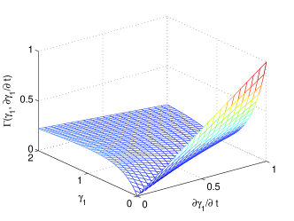
Figure 1: Character function $\Gamma$ versus $\gamma_{1}(T)$ and $\frac{\partial}{\partial t}\gamma_{1}(T)$ at a fixed time point $T$. $\gamma_{1}$ describes the decay rate of the system, whereas $\frac{\partial}{\partial t}\gamma_{1}$ characterizes the change rate of $\gamma_{1}$. Both $\gamma_{1}$ and $\frac{\partial}{\partial t}\gamma_{1}$ can vary independently, for example when $\gamma_{1}=\omega t$, $\frac{\partial}{\partial t}\gamma_{1}=\omega$. The other parameters chosen are $\gamma_{2}=1$ and $\frac{\partial}{\partial t}\gamma_{2}=1.$

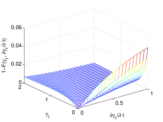
Figure 2: The fidelity ($1-\mathcal{F}$) as functions of $\gamma_{1}$ and $\frac{\partial}{\partial t}\gamma_{1}.$ The other parameters are the same as in Fig. 1

In the context of effective Hamiltonian approach, we now formulate the dynamically stable decoherence-free subspaces for the non-Markovian dynamics governed by Eq.(39). In terms of the wave function vector $\overrightarrow{|\mathbf{\Psi}(t)\rangle}=\left[|\Psi_{1}(t)\rangle,|\Psi_{2}(t)\rangle,\cdots\right]^{\mathbf{T}},$ the definition of DDFSs given in Eq.(27) can be expressed as

$$\sum_{i,j}\frac{\partial}{\partial t}\langle\Psi_{i}(t)|\Psi_{j}(t)\rangle=0,\ \forall t\geq 0,\ \$$

$$\mbox{with}\ \ \sum_{i,j}\langle\Psi_{i}(0)|\Psi_{j}(0)\rangle=1.$$ (57)

By the Schrödinger -like equation Eq.(42), this definition immediately follows,

$$\sum_{ijk}\langle\Psi_{i}|\mathbf{H}_{jk}-\tilde{{\mathbf{H}}}^{*}_{ji}|\Psi_{k}\rangle=0.$$ (58)

If $R_{kj}^{\lambda}|\Phi_{m}\rangle=\beta_{k}^{\lambda}|\Phi_{m}\rangle$ holds for all $\lambda,k,j$ and the eigenvalue $\beta_{k}^{\lambda}$ is independent of $m$ and $j$, we have $\sum_{i,j}\frac{\partial}{\partial t}\langle\Psi_{i}(t)|\Psi_{j}(t)\rangle=0,$ namely $\mathcal{H}^{\prime}_{DDFSs}\equiv\{|\Phi_{m}\rangle\}$ composes a DDFSs. With $R_{kj}^{\lambda}|\Phi_{m}\rangle=\beta_{k}^{\lambda}|\Phi_{m}\rangle$, the elements of the effective Hamiltonian matrix reduce to

$$H_{kj}^{DDFSs} = \delta_{kj}(H_{k}-\frac{i}{2}\sum_{p\lambda}\beta_{p}^{\lambda}R_{pk}^{\lambda\dagger}-H_{k}^{A}+\frac{i}{2}\sum_{p\lambda}\beta_{p}^{\lambda*}R_{pk}^{\lambda A\dagger})$$ (59)

$$+ i\sum_{\lambda}\beta_{k}^{\lambda}R_{kj}^{\lambda A}.$$

Thus that $\mathcal{H}^{\prime}_{DDFSs}$ is invariant under the effective Hamiltonian with matrix elements $H_{kj}^{DDFSs}$ is required. We observed that these conditions are similar to that in Eqs (31,32), so by repeating the same procedure, we can prove that these conditions are necessary for DDFSs.

VI Conclusion and Discussion

Based on the effective Hamiltonian approach, we have presented a self-consistent framework for the analysis of geometric phases and dynamically stable decoherence-free subspaces in open systems. Comparisons to the earlier works are made. A connection of this effective Hamiltonian approach to the method based on the damping basis has been established. This effective Hamiltonian approach is then extended to a non-Markovian case with the generalized Lindblad master equation. As an example, the non-Markovian master equation describing a dissipative two-level system has been solved by this method. An adiabatic evolution has been defined and the corresponding adiabatic condition has been given based on this extended effective Hamiltonian approach. A necessary and sufficient condition for the dynamically stable decoherence-free space is also presented. The effective Hamiltonian approach can be extended to all master equations which are local in time. The geometric phase defined through the effective Hamiltonian is in fact a difference of two geometric phases, when the system under consideration is a closed system with pure initial states. The present analysis is available for all master equations that are local in time, i.e., at any point in time the future evolution only depends on the present state and not on the history of the system. We restrict ourself in this paper to consider the case where the effective Hamiltonian is diagonalizable and its eigenstates are nondegenerate. The situation beyond this limitation can be analyzed by introducing Jordan blocks in the Hamiltonian, which beyond the scope of this paper.

This work is supported NUS Research Grant WBS:R-710-000-008-271 and NSF of China under grant Nos. 60578014 and 10775023.

Appendix: Eigenstates and The Corresponding Eigenvalues of The Effective Hamiltonian Matrix

In this section, we list the eigenstates and the corresponding eigenvalues for the effective Hamiltonian matrix $\mathbf{H}$. The eight eigenvalues are, $0$ (threefold degenerate, corresponding to $A^{01},A^{02},A^{03}$), $-\frac{\gamma_{1}}{2}i$ (twofold degenerate corresponding to $A^{11},A^{12}$), $-\frac{\gamma_{2}}{2}i$ (twofold degenerate corresponding to $A^{21},A^{22}$), and $-(\gamma_{1}+\gamma_{2})$ (corresponding to $A^{3}$). The corresponding right eigenstates are (in damping basis)

$$A^{01}=\left\{A^{01}_{1}=0,A^{01}_{2}=|e\rangle\langle e|\right\},$$

$$A^{02}=\left\{A^{02}_{1}=|g\rangle\langle g|,A^{02}_{2}=0\right\},$$

$$A^{03}=\left\{A^{03}_{1}=\frac{\gamma_{1}}{\gamma_{1}+\gamma_{2}}|e\rangle\langle e|,A^{03}_{2}=\frac{\gamma_{2}}{\gamma_{1}+\gamma_{2}}|g\rangle\langle g|\right\},$$

$$A^{11}=\left\{A^{11}_{1}=0,A^{11}_{2}=|g\rangle\langle e|\right\},$$

$$A^{12}=\left\{A^{12}_{1}=0,A^{12}_{2}=|e\rangle\langle g|\right\},$$

$$A^{21}=\left\{A^{21}_{1}=|g\rangle\langle e|,A^{21}_{2}=0\right\},$$

$$A^{22}=\left\{A^{22}_{1}=|e\rangle\langle g|,A^{22}_{2}=0\right\},$$

$$A^{3}=\left\{A^{3}_{1}=|e\rangle\langle e|,A^{3}_{2}=-|g\rangle\langle g|\right\},$$

and their dual

$$B^{01}=\left\{B^{01}_{1}=0,B^{01}_{2}=|e\rangle\langle e|\right\},$$

$$B^{02}=\left\{B^{02}_{1}=|g\rangle\langle g|,B^{01}_{2}=0\right\},$$

$$B^{03}=\left\{B^{03}_{1}=|e\rangle\langle e|,B^{03}_{2}=|g\rangle\langle g|\right\},$$

$$B^{11}=\left\{B^{11}_{1}=0,B^{01}_{2}=|e\rangle\langle g|\right\},$$

$$B^{12}=\left\{B^{12}_{1}=0,B^{12}_{2}=|g\rangle\langle e|\right\},$$

$$B^{21}=\left\{B^{21}_{1}=|e\rangle\langle g|,B^{21}_{2}=0\right\},$$

$$B^{22}=\left\{B^{22}_{1}=|g\rangle\langle e|,B^{22}_{2}=0\right\},$$

$$B^{3}=\left\{B^{3}_{1}=\frac{\gamma_{2}}{\gamma_{1}+\gamma_{2}}|e\rangle\langle e|,B^{3}_{2}=-\frac{\gamma_{1}}{\gamma_{1}+\gamma_{2}}|g\rangle\langle g|\right\}.$$

The alternative expressions can be given in the Hilbert space spanned by $\{|ee\rangle,|eg\rangle,|ge\rangle,|gg\rangle\}$

$$A^{01}_{1}=\left[0,0,0,0\right]^{\mathbf{T}},\ A^{01}_{2}=\left[1,0,0,0\right]^{\mathbf{T}},$$

$$A^{02}_{1}=\left[0,0,0,1\right]^{\mathbf{T}},\ A^{02}_{2}=\left[0,0,0,0\right]^{\mathbf{T}},$$

$$A^{03}_{1}=\left[\frac{\gamma_{1}}{\gamma_{1}+\gamma_{2}},0,0,0\right]^{\mathbf{T}},\ A^{03}_{2}=\left[0,0,0,\frac{\gamma_{2}}{\gamma_{1}+\gamma_{2}}\right]^{\mathbf{T}},$$

$$A^{11}_{1}=\left[0,0,0,0\right]^{\mathbf{T}},\ A^{11}_{2}=\left[0,0,1,0\right]^{\mathbf{T}},$$

$$A^{12}_{1}=\left[0,0,0,0\right]^{\mathbf{T}},\ A^{12}_{2}=\left[0,1,0,0\right]^{\mathbf{T}},$$

$$A^{21}_{1}=\left[0,0,1,0\right]^{\mathbf{T}},\ A^{21}_{2}=\left[0,0,0,0\right]^{\mathbf{T}},$$

$$A^{22}_{1}=\left[0,1,0,0\right]^{\mathbf{T}},\ A^{22}_{2}=\left[0,0,0,0\right]^{\mathbf{T}},$$

$$A^{3}_{1}=\left[1,0,0,0\right]^{\mathbf{T}},\ A^{3}_{2}=\left[0,0,0,-1\right]^{\mathbf{T}},$$

are the right eigenstates, and

$$B^{01}_{1}=\left[0,0,0,0\right],\ B^{01}_{2}=\left[1,0,0,0\right],$$

$$B^{02}_{1}=\left[0,0,0,1\right],\ B^{02}_{2}=\left[0,0,0,0\right],$$

$$B^{03}_{1}=\left[1,0,0,0\right],\ B^{03}_{2}=\left[0,0,0,1\right],$$

$$B^{11}_{1}=\left[0,0,0,0\right],\ B^{11}_{2}=\left[0,0,1,0\right],$$

$$B^{12}_{1}=\left[0,0,0,0\right],\ B^{12}_{2}=\left[0,1,0,0\right],$$

$$B^{21}_{1}=\left[0,0,1,0\right],\ B^{21}_{2}=\left[0,0,0,0\right],$$

$$B^{22}_{1}=\left[0,1,0,0\right],\ B^{22}_{2}=\left[0,0,0,0\right],$$

$$B^{3}_{1}=\left[\frac{\gamma_{2}}{\gamma_{1}+\gamma_{2}},0,0,0\right],B^{3}_{2}=\left[0,0,0,-\frac{\gamma_{1}}{\gamma_{1}+\gamma_{2}}\right],$$

are the left eigenstates.

References

- (1) A. Kossakowski, Rep. Math. Phys 3, 247 (1972).
- (2) V. Gorini, A. Kossakokowski, and E. C. G. Sudarshan, J. Math. Phys 17, 821 (1976).
- (3) G. Lindblad, Commun. Math. Phys. 48, 119 (1976).
- (4) M. O. Scully and M. S. Zubairy Quantum Optics (Cambridge University Press, Cambridge 1997); D. F. Walls and G. J. Milburn Quantum Optics (Springer, Berlin,1994).
- (5) M. A. Nielsen and I. L. Chuang Quantum computation and quantum information (Cambridge University Press, Cambridge, England, 2000).
- (6) L. M. Arévalo-Aguilar and H. Moya-Cessa, Quantum Semiclassic. Opt. 10 671 (1998).
- (7) A. B. Klimov and J. L. Romero, J. Opt. B, 5, S316 (2003);
- (8) H. Nakazato, Y. Hida, K. Yuasa, B. Militello, A. Napoli, and A. Messina, Phys. Rev. A 74, 062113 (2006).
- (9) J. Yang, Y. D. Zhang, and Z. B. Chen, Phys. Rev. A 67, 024101 (2003).
- (10) J. Yang, H. X. Lu, B. Zhao, M. S. Zhao, and Y. D. Zhang, Chin. Phys. Lett. 20, 796 (2003).
- (11) X. X. Yi, C. Li, and J. C. Su Phys. Rev. A 62, 013819 (2000).
- (12) H. J. Briegel and B. G. Englert, Phys. Rev. A 47, 3311 (1993).
- (13) X. X. Yi and S. X. Yu, J. Opt. B, 3, 372 (2001).
- (14) E. Hahn, Phys. Rev. 80, 580 (1950).
- (15) R. I. Karasik, K. P. Marzlin, B. C. Sanders, and K. B. Whaley, Phys. Rev. A 77, 052301 (2008).
- (16) G. Engel, T. Calhoun, E. Read, T. Ahn, T. Mancal, Y. Cheng, R. Blankenship, and G. Fleming, Nature 446, 782 (2007).
- (17) A. Shabani and D. A. Lidar, Phys. Rev. A 71, 020101(R) (2005).
- (18) C. Uchiyama, Phys. Lett. A 356, 294 (2006).
- (19) S. M. Barnett and S. Stenholm, Phys. Rev. A 64, 033808 (2001).
- (20) S. Maniscalco, Phys. Rev. A 75, 062103 (2007).
- (21) A. Shabani and D. A. Lidar, Phys. Rev. A 71, 020101(R) (2005).
- (22) X. L. Huang, J. Nie, J. Chen and X. X. Yi, Phys. Scr. 78, 025001 (2008).
- (23) S. Maniscalco and F. Petruccione, Phys. Rev. A 73, 012111 (2006).
- (24) H. P. Breuer, Phys. Rev. A 75, 022103 (2007).
- (25) H. P. Breuer, J. Gemmer, and M. Michel, Phys. Rev. E 73, 016139 (2006).
- (26) H. P. Breuer: Non-Markovian quantum dynamics and the method of correlated projection superoperators, arXiv: quan-ph/0707.0172.
- (27) E. Ferraro, H.-P. Breuer, A. Napoli, M. A. Jivulescu, and A. Messina, Phys. Rev. B 78,064309 (2008).
- (28) B. Vacchini, Phys. Rev. A 78, 022112 (2008).
- (29) H. P. Breuer and F. Petruccione, The Theory of Open Quantum Systems (Oxford University Press, Oxford 2002).
- (30) X. X. Yi, D. M. Tong, L. C. Kwek, and C. H. Oh, J. Phys. B 40, 281 (2007).
- (31) M. S. Sarandy, E. I. Duzzioni, and M. H. Y. Moussa, Phys. Rev. A 76, 052112(2007).
- (32) M. S. Sarandy and D. A. Lidar, Phys. Rev. A 71, 012331 (2005).
- (33) A. V. Sokolov, A. A. Andrianov, and F. Cannata, e-print: quant-ph/0602207.
- (34) G. M. Palma, K.-A. Suominen, and A. K. Ekert, Proc. Roy. Soc. London Ser. A 452, 567 (1996).
- (35) L. M. Duan and G. C. Guo, Phys. Rev. Lett. 79, 1953 (1997).
- (36) L. M. Duan and G. C. Guo, Phys. Rev. A 57, 737 (1998).
- (37) P. Zanardi and M. Rasetti, Phys. Rev. Lett. 79, 3306 (1997).
- (38) D. A. Lidar, I. L. Chuang, and K. B. Whaley, Phys. Rev. Lett. 81, 2594 (1998).
- (39) E. Knill, R. Laflamme, and L. Viola, Phys. Rev. Lett. 84, 2525 (2000).
- (40) X. L. Huang, H. Y. Sun, and X. X. Yi, Phys. Rev. E 78, 04**** (2008). To be published.
- (41) J. Gemmer, M. Michel, and G. Mahher, Quantum Thermodynamics Lecture Notes in Physics. Vol.657 (Springer-Verlag, Berlin 2004).
- (42) J. Gemmer and M. Michel, Europhysics Letters 73, 1 (2006).
- (43) M. Born and V. Fork, Z. Phys. 51, 165 (1928).
- (44) For a general system, this condition is not sufficient. Nevertheless, for the example given below, this is a good condition for the adiabaticity, as shown below. For recent progresses in this direction for closed systems, please read, K. P. Marzlin, B. C. Sanders, Phys. Rev. Lett. 93, 160408(2004); D. M. Tong et al., Phys. Rev. Lett. 95 110407(2005). As shown, this condition may not be sufficient for some special systems, however, it is powerful in most cases. So does Eq.(55).
- (45) D. Bures, Tran. Am. Math. Soc. 135, 199 (1969); A. Uhlmann, Rep. Math. Phys. 9, 273 (1976); M. Hübner, Phys. Lett. A 163, 229 (1992); R. Jozsa, J. Mod. Opt. 41, 2315 (1994); B. Schumacher, Phys. Rev. A 51, 2738 (1995).