Topological quantum numbers and curvature — examples and applications

Abstract

Using the idea of the degree of a smooth mapping between two manifolds of the same dimension we present here the topological (homotopical) classification of the mappings between spheres of the same dimension, vector fields, monopole and instanton solutions. Starting with a review of the elements of Riemannian geometry we also present an original elementary proof of the Gauss-Bonnet theorem and the Poincaré-Hopf theorem.

1 Introduction

From the beginning of the first half of the 1970s we can observe the growing importance of the topological (global) methods of analysing the structures of solutions of nonlinear equations of mathematical physics [1].

In this article we discuss first the very important idea of the degree of a smooth mapping between smooth manifolds, a homotopical invariant which is very useful for the above mentioned methods.

We describe the fundamental properties of degree of a smooth mapping between the manifolds of the same dimension. In relatively simple way we introduce the integral formula for the mapping degree and in a systematic way we present explicit formulas for the degree of the mapping between the $n$-dimensional spheres.

We then determine, in a new way, the explicit formulas for the index of vector field in relation to hypersurfaces and to point. The novelty of our approach lies in an effective use of differential forms.

Using the idea of an index of a vector field we then present a formula for the topological quantum number characterizing monopole configurations in the Yang-Mills-Higgs theory with gauge group $SU(2)$. Using the idea of an index of a vector field we derive the formula for a “topological quantum number” (Chern number) characterizing homotopically nonequivalent instanton configurations of Yang-Mills theory with gauge group $SU(2)$. We show also the bijectivity between the elements of the $SU(2)$ gauge group and unit vector fields on $R^{4}$

After introducing the elements of Riemannian geometry we present an original, elementary proofs of Gauss-Bonnet and Poincaré-Hopf theorems for compact, closed, oriented, two-dimensional manifolds. The traditional proof of the Gauss-Bonnet theorem uses classical geometry and is much more complicated. Proving the Gauss-Bonnet theorem we used effective language of the differential forms and skilfully used the notion of the form of connection. The new ingredient in the proof of the Poincaré-Hopf theorem is the expression of an index of the vector field at a point by suitable scalar products (formula (23) below). This line of proof (after a generalization to higher dimensions) creates a possibility of formulation a sufficient condition for the existence of a pseudo-Riemannian metric on compact manifolds without a boundary. Such a condition would be very useful in modern cosmology. Finally we discuss the Poincaré-Hopf theorem for any even dimensional compact orientable manifold without boundary.

Instantons are very interesting both from the physical and mathematical point of view. They are topologicaly nontrivial solutions of Yang-Mills equations which globally minimized in chosen topological class of a functional of euclidean action. One can use them to analyze tunneling processes occurring in different systems, e.g. in Yang-Mills theory and in the system described by nonrelativistic quantum mechanics [2] The topological characterization of monopoles and instantons, presented in this paper, might be useful in many applications. To remind the importance of monopoles in physics, let us mention that the so called ’monopole problem’ was a direct motivation for the inflationary models in cosmology [3], and that monopoles can catalyse the decay of a proton [4].

In addition, this work presents an elementary topological classification of two-dimensional surfaces via a heuristic proof of the Gauss-Bonnet theorem. Such classifications are commonly used in string theory.

2 The basic definitions

2.1 Critical points of the mapping

We will consider a smooth mapping $f\colon M\to N$ between the smooth manifolds $M$ and $N$. By $C_{f}$ we denote the collection of points $p\in M$ such that differential (tangent mapping) $d_{p}f\colon T_{p}M\to T_{f(p)}N$ has a smaller rank than the dimension of the manifold $N$:

$$C_{f}=\left\{{p\in M\colon rk\left({d_{p}f}\right)<\dim N}\right\}$$

Here the set $C_{f}$ is the set of the critical points of the $f$ mapping and the set $f(C_{f})$ is the set of the critical values of this mapping.
Definition
The set $A\subset R^{n}$ is called the set of the null measure in $R^{n}$ if one can cover it with a countable family of the $n$-dimensional cubes with the arbitrary, small total volume of that cover. We can generalize the definition of the set of the null measure also for subsets of the smooth manifolds, namely the subset $A\subset M$, where $M$ is $n$-dimensional smooth manifold with the atlas $\left\{{(U_{i},\phi_{i})}\right\}$.
We say that $A$ has a null measure if for any coordinate mapping $\phi_{i}:U_{i}\to R^{n}$ the image $\phi_{i}\left({U_{i}\cap A}\right)$ has a null measure set in $R^{n}$. The fundamental Sard’s theorem says [5]: Let $f\colon M\to N$ be the smooth mapping of the smooth manifolds $M$ and $N$. Then the set of the critical value $f(C_{f})$ of this mapping is the null measure set in $N$.

A point $p\in M$ is called a regular point of the smooth mapping $f\colon M\to N$ if it is not the critical point, i.e. when $rk(d_{p}f)=\dim N$.

A point $q\in N$ is called a regular value of the mapping $f\colon M\to N$ if all points $p_{a}\in M$ belonging to the inverse image $f^{-1}(\left\{q\right\})$ of the point $q$ are the regular points of the mapping $f$. (When $f^{-1}\left({\left\{q\right\}}\right)=$ $\emptyset$ then the point $q$ we call the regular value of the mappings $f$.)

2.2 Homotopy

The smooth (continuous) homotopy of the mapping $f\colon M\to N$ we call the smooth (continuous) mapping $F$ of the cylinder $M\times\left[{0,1}\right]$ in manifold $N$ i.e. $F\colon M\times\left[{0,1}\right]\to N$ such that $F(p,0)=f(p)$ for any point $p\in M$.

About the mappings $f_{t}\colon M\to N$ where $f_{t}(p)=F(p,t)$ we say that they are homotopic with the ”initial” mapping $f_{0}=f$. For any mapping of the cylinder $M\times[0,1]$ we say that it is the homotopy or the homotopy process between the mappings $f_{0}$ and $f_{1}$ where $f_{1}(p)=F(p,1)$. We say two mapping $f_{0}$ and $f_{1}$ are homotopic when there is the homotopy between them.

The set of points of the form $(p,0)$ we call the base of the cylinder while the set of points of the form $(p,1)$ we call its bottom.

Therefore two mappings $f_{0}\colon M\to N$ and $f_{1}\colon M\to N$ are homotopic if there exists a smooth (continuous) mapping of the cylinder over $M$ that extends the map defined by $f_{0}$ at the bottom of the cylinder and by $f_{1}$ defined at the top. The same way all mappings from $M$ to $N$ share homotopy classes, and each class consists of the mappings homotopic with one another. The set of homotopy classes of the mappings from $M$ into $N$ we denote by $\left\{{M,N}\right\}$.

Definition
Two manifolds $M$ and $N$ we call homotopicaly equivalent if there exist the smooth mappings $f\colon M\to N$ and $g\colon N\to M$ such that the composite mappings $g\circ fcolonM\to M$ and $f\circ g\colon N\to N$ are homotopic with the identity mappings. If the manifolds $M$ and $N$ are homotopicaly equivalent then for any manifold $P$ there exists a bijection between their respective homotopy classes $\left\{{P,M}\right\}$ and $\left\{{P,N}\right\}$.

2.3 Degree of mapping

The degree of mapping is a quantity with which we are able to consider the homotopy classes among the manifolds: closed (i.e. compact and without boundaries), oriented, $M$ and $N$ with the same dimension; $\dim M=\dim N$.

Lets consider the smooth mapping $f\colon M\to N$ and fix a point $q_{0}\in N$. We will assume that the mapping $f\colon M\to N$ is the proper mapping in relation to the point $q_{0}$ i.e. the inverse image $f^{-1}\left({\left\{{q_{0}}\right\}}\right)$ consists of the finite number of points $f^{-1}\left({\left\{{q_{0}}\right\}}\right)=\left\{{p_{1},\ldots,p_{R}}\right\}\subset M$ and for $a=1,\ldots,R$, $\det[d_{p_{a}}f]\neq 0$.

Definition
The degree of the smooth mapping $f\colon M\to N$ $(\deg f)$ of the connected manifolds, closed, oriented, possessing the same dimension, is defined by an integer

$$\deg f=\sum\limits_{p_{a}\in f^{-1}\left({\left\{{q_{0}}\right\}}\right)}{{\mathop{\rm sgn}}[\det\left({d_{p_{a}}f}\right)}]$$ (1)

($f$ is the proper mapping in the relation to the point $q_{0}$).

The degree of the mapping we call also the algebraic number of inverse image. We quote without the proof the very important theorem of the degree of mapping:

Theorem
The mapping degree does not depend on the choice of the regular value $q_{0}$ and is invariant under a homotopy process i.e. does not change with the homotopy of the given mapping—in other words—it is the characteristics of the element belonging to the set $\left\{{M,N}\right\}$.

Heuristically, the homotopical invariance of the degree can be shown via a continuity argument. Namely, the degree, by definition, takes integer values and is a continuous function of a deformation parameter t, hence it must be a constant function of this parameter. It is clear from the integral formula for the degree that it is independent of the choice of a regular value of the mapping.

Moreover, the following theorem is true: Two smooth mappings $f$ and $g$ : $M\to S^{n}$ of an $n$-dimensional closed, oriented manifold $M$ to the $n$-dimensional sphere $S^{n}$ are homotopic if and only if (iff) when their degrees overlie [5].

3 Integration of the form and degree of mapping

We will show that the degree of the mapping can be specified by integrating the proper differential forms over the manifolds. Let us consider the behavior of the integral of the differential $n$-form $\omega$ over a $n$-dimensional closed and oriented manifold which respect to the mapping $f$ with the specified degree. Let $M$ and N be the manifolds of the same dimension n, closed and oriented and let $f\colon M\to N$ be the smooth mapping having the specified degree denoted by $\deg f$ and let $\omega$ be the differential $n$-form on $M$. We have the following formula:

$$\int\limits_{M}{f^{*}}\omega=\deg f\int\limits_{N}\omega,$$ (2)

where $f^{*}\omega$ is the pull-back of the form $\omega$ on the manifolds $M$ by the mapping $f$.
Sketch of the proof:
Let us choose in $N$ the regular value $q_{0}$ of the mapping $f$. Lets $\hat{V}$ denote the neighborhood of the point $q_{0}$ which is created by the points being the regular values of the mapping $f$.
Let the inverse image $f^{-1}\left({\left\{{q_{0}}\right\}}\right)$ consists of the regular points $p_{1}^{0},\ldots,p_{R}^{0}$ of mapping $f$. The neighborhoods of these points $\hat{U}_{1},\ldots,\hat{U}_{R}$ is the inverse image of the set $\hat{V}$ : $f^{-1}(\hat{V})=\hat{U}_{1}\cup\hat{U}_{2}\cup\ldots\cup\hat{U}_{R}$.

Every neighborhood $\hat{U}_{a}$ $a=1,2,\ldots,R$ consists of the regular points of mapping $f$ and the subsets $\hat{U}_{a}$ with a suitable choice of the neighborhood are disjoint.
On manifolds $M$ and $N$ we always choose the coordinate mappings such that the disjoint coordinate neighborhoods $U_{a}$ $(a=1,2,\ldots,R)$ fulfill the conditions $\hat{U}_{a}\subset U_{a}$.

The mappings $\phi_{a}\colon U_{a}\to$ $R^{n}$ define in the manifold $M$ local coordinates $\phi_{a}(p)=\left({x_{a}^{1},\ldots,x_{a}^{n}}\right)$ of point $p\in U_{a}$. Likewise, on manifold $N$ we choose the coordinate neighborhood $V$ in such a way that $\hat{V}\subset V$, with local coordinates defined by the mapping $\psi\colon V\to R^{n}$ denoted by $\left({y^{1},\ldots,y^{n}}\right)=\psi(q)$ for $q\in V$. In local coordinates $\left({y^{1},\ldots,y^{n}}\right)$ the differential $n$-form $\omega$ has the form $\omega=g\left({y^{1},\ldots,y^{n}}\right)dy^{1}\wedge dy^{2}\wedge\ldots\wedge dy^{n}$ where $g$ is a smooth real-valued function.

The pull-back form $f^{*}\omega$ in neighborhood of point $p_{a}^{0}$ in local coordinates has the form:

$$f^{*}\omega\left|{{}_{\hat{U}_{a}}}\right.=g\circ f\det\left[\frac{{\partial f^{\mu}}}{{\partial x_{a}^{\nu}}}(x_{a})\right]dx_{a}^{1}\wedge\ldots\wedge dx_{a}^{n}.$$

The restriction of a mapping $f$ to subset $\hat{U}_{a}$ is the diffeomorphism $f\colon\hat{U}_{a}\to\hat{V}$. Hence:

$$\int\limits_{\hat{U}_{a}}{f^{*}}\omega = \int\limits_{\phi_{a}(\hat{U}_{a})}{g(f(x_{a})})\det\left[\frac{{\partial f^{\mu}}}{{\partial x_{a}^{v}}}(x_{a})\right]dx_{a}^{1}\wedge\ldots\wedge dx_{a}^{n}$$

$$= {\mathop{\rm sgn}}\left[\det\left({{\frac{\partial f^{\mu}}{\partial x_{a}^{\nu}}(p_{a}^{0})}}\right)\right]\int\limits_{\phi_{a}(\hat{U}_{a})}{g\left({f(x_{a})}\right)}\left|{\det\left[\frac{{\partial f^{\mu}}}{{\partial x_{a}^{\nu}}}(x_{a})\right]}\right|{dx_{a}^{1}\ldots dx_{a}^{n}}^{n}$$

$$= {\mathop{\rm sgn}}\left[\det\left({\frac{\partial f^{\mu}}{\partial x_{a}^{\nu}}(p_{a}^{0})}\right)\right]\int\limits_{\psi(\hat{V})}{g(y^{1}},\ldots,y^{n})dy^{1}\ldots dy^{n}$$

$$= {\mathop{\rm sgn}}\left[\det(d_{p_{a}^{0}}f)\right]\int\limits_{\hat{V}}\omega,$$

where we used the fact that on the set $\phi_{a}(U_{a})$ the sign of the determinant $\det\left({\frac{{\partial f^{\mu}}}{{\partial x_{a}^{\nu}}}(x_{a})}\right)$ is constant and we made use of the theorem on the change of variables in a multiple integral. Hence:

$$\int\limits_{f^{-1}(\hat{V})}{f^{*}}\omega=\sum\limits_{a=1}^{R}{\int\limits_{\hat{U}_{a}}{f^{*}}}\omega=\left[{\sum\limits_{a=1}^{R}{{\mathop{\rm sgn}}\left({\det(d_{p_{a}}f)}\right)}}\right]\int\limits_{\hat{V}}\omega.$$

In other words:

$$\int\limits_{f^{-1}(\hat{V})}{f^{*}}\omega=\deg f\int\limits_{\hat{V}}\omega$$

If this form $\omega$ has the values different from zero only on the set $\hat{V}$, then $\int\limits_{\hat{V}}\omega=\int\limits_{N}\omega$ and $\int\limits_{f^{-1}(\hat{V})}{f^{*}}\omega=\int\limits_{M}{f^{*}\omega}$ so for this form:

$$\int\limits_{M}{f^{*}}\omega=\deg\int\limits_{N}\omega.$$

If we have any $n$-form defined on manifold $N$ we will see that on set $C_{f}\subset M$ form $f^{*}\omega$ is equal to zero so $\int\limits_{M}{f^{*}\omega}=\int\limits_{M\backslash C_{f}}{f^{*}\omega}$. According to Sard’s theorem the set $f(C_{f})$ is the set of the null measure in $N$ so

$$\int\limits_{N}{\omega=\int\limits_{N\backslash f(C{}_{f})}\omega}.$$

Let $\left\{{\alpha_{i}}\right\}$ be a partition of unity subordinated to the covering $\left\{{V_{i}}\right\}$ of the manifold $N\backslash f(C_{f})$. Then the form $\alpha_{i}\omega$ has the value of null outside the set $V_{i}$ and $\int\limits_{M}{f^{*}(\alpha_{i}}\omega)=\deg f\int\limits_{M}{\alpha_{i}}\omega$. After summation of the last equation with respect to $i$ we get:

$$\int\limits_{M\backslash C_{f}}{f^{*}\omega=\deg f\int\limits_{N\backslash f(C_{f})}\omega},$$

because: $\sum\limits_{i}{\alpha_{i}}=1$, $f^{*}\left({\alpha_{i}\omega}\right)=(\alpha_{i}\circ f)f^{*}\omega$ and $\sum\limits_{i}{\alpha_{i}}\left({f(p)}\right)=1$. This concludes the proof of the theorem.

Let us remark that if $N$ is the closed manifold and $\eta$ is the volume form on $N$ i.e. when $\int\limits_{N}\eta=volN$ and $f\colon M\to N$ is the smooth mapping between the closed and oriented manifolds of the same dimension then: $\int\limits_{M}{f^{*}}\eta=\deg f\int\limits_{N}{\eta=\deg f(volN})$, hence:

$$\deg f=\frac{1}{{volN}}\int\limits_{M}{f^{*}}\eta$$ (3)

This integral formula provides an effective method to determine the degree of the mapping.

4 Some applications of integral formula of degree of mapping

4.1 Solid angle form and spheres mapping

In domain $R^{n+1}\backslash\left\{0\right\}$ which is homotopicaly equivalent with the sphere $S^{n}$ lets consider the following $n$-form:

$$\Omega_{n}=\frac{1}{{vol(S^{n})}}\frac{{\sum\limits_{\alpha=1}^{n+1}{(-1)^{\alpha-1}x^{\alpha}dx^{1}\wedge\ldots\wedge d\mathop{x^{\alpha}}\limits^{\vee}\wedge\ldots\wedge dx^{n+1}}}}{{\left[{(x^{1})^{2}+\ldots+(x^{n+1})^{2}}\right]^{\frac{{n+1}}{2}}}}$$ (4)

where symbol ”$\vee$” put over an object means that this object is omitted, $vol(S^{n})$ is the area of the $n$-dimensional sphere:

$$vol(S^{n})=\left\{{\begin{array}[]{*{20}l}{\frac{{2\pi^{r+1}}}{{r!}}-for-n=2r+1}\\ \\ {\frac{{2^{r+1}\pi^{r}}}{{\left({2r-1}\right)!!}}-for-n=2r}\\ \end{array}}\right.$$

It is easy to see that the form $\Omega_{n}$ is the closed form i.e. $d\Omega_{n}=0$ but it is not the exact form because $\int\limits_{S^{n}}{\Omega_{n}}=1$ where $S^{n}$ is the $n$-dimensional sphere given by the equation $(x^{1})^{2}+\ldots+(x^{n+1})^{2}=1$. The form $\Omega_{n}$ is distinguished in the domain $R^{n+1}\backslash\left\{0\right\}$ in the sense that any closed $n$-form defined in this domain has the form $Q\Omega_{n}+d\alpha$, where $Q$ is the real number and $\alpha$ is some $(n-1)$ differential form.

The geometrical meaning of the form $\Omega_{n}$ is as follows: If some $n$-dimensional hypersurface $M^{n}$ in $R^{n+1}$ is given by the immersion $\phi\colon R^{n}$ $\supset U\to M^{n}$ i.e. by the mapping $\underbrace{\left({t^{1},t^{2},\ldots,t^{n}}\right)}_{\in U}=t\mapsto\left({x^{1}(t),\ldots x^{n+1}(t)}\right)\in M^{n}$, then the integral $\int\limits_{U}{\phi^{*}\Omega_{n}}$ says what fraction of the total solid angle is covered by the hypersurface $M^{n}$ when we look at it from the point $0$. An example: for $n=2$ we have:

$$\Omega_{2} = \frac{1}{{4\pi}}\frac{{xdy\wedge dz+ydz\wedge dx+zdx\wedge dy}}{{\left|{\vec{r}}\right|^{3}}},$$

$$\phi^{*}\Omega_{2}(t^{1},t^{2}) = \frac{1}{{4\pi}}\frac{{\vec{r}(t)\cdot\vec{n}(t)}}{{\left|{\vec{r}(t)}\right|^{3}}}\left|{\vec{E}_{1}\times\vec{E}_{2}}\right|dt^{1}\wedge dt^{2},$$

where $\vec{E}_{a}(t)=\frac{{\partial\vec{r}}}{{\partial t^{a}}}(t^{1},t^{2})$ $(a=1,2)$ are vectors tangent to surface in $\vec{r}(t)$ point when $\vec{n}(t)=\frac{{\vec{E}_{1}(t)\times\vec{E}_{2}(t)}}{{\left|{\vec{E}_{1}\times\vec{E}_{2}}\right|}}$ is the unit normal vector to surface in point $\vec{r}(t)$.

Thus the form $\Omega_{n}$ can be called the normalized solid angle form.

The circle $S^{1}$ is defined by the standard immersion: $\phi\colon\underbrace{\varphi}_{\varphi\in R}\mapsto(\cos\varphi,\sin\varphi)$. Let us notice that $\phi^{*}\Omega_{1}(\varphi)=\frac{1}{{2\pi}}d\varphi=\frac{1}{{2\pi}}\eta$ where $\eta$ is the circle volume form. Points $\varphi$ and $\varphi+2m\pi$ where $m\in$ Z indeed define the same point on the circle. Mapping of circle $S^{1}$ into circle $S^{1}$ we will get as the result of composition of mappings $\phi\circ f$, where $f$ is such smooth function $f\colon R\to R$ so $f(\varphi+2\pi)=f(\varphi)+2n\pi$, where $n\in$ Z. Lets notice too that $\phi\circ f\colon\varphi\mapsto\phi\left({f(\varphi)}\right)=\left({\cos f(\varphi),\sin f(\varphi)}\right)$ and $\left({\phi\circ f}\right)^{*}\Omega_{1}=f^{*}\circ\phi^{*}\Omega_{1}=\frac{1}{{2\pi}}f^{*}\eta=\frac{1}{{2\pi}}f^{\prime}(\varphi)d\varphi$ so the degree of mapping of a circle into a circle is given by the formula:

$$\deg f=\frac{1}{{2\pi}}\int\limits_{0}^{2\pi}{f^{\prime}(\varphi)d\varphi=\frac{1}{{2\pi}}}[f(2\pi)-f(0)]=n.$$ (6)

For example if $f_{n}(\varphi)=n\varphi$; $n\in$ Z then obviously $\deg f_{n}=n$. It is to be easily seen that for such a mapping the image of the circle $S^{1}$ $n$-times ”winds” on the circles $S^{1}$. That is the reason why number $n$ is called the winding number. Each mapping of a circle into a circle is homotopicaly equivalent to some mapping $f_{n}$.

So the set of all homotopy classes $\left\{{S^{1},S^{1}}\right\}$ is bijective with the set of integer numbers, Z. Analogously the set of all homotopy classes $\left\{{S^{n},S^{n}}\right\}$ is bijective with the set of integer numbers Z.

Let us consider now $2$-dimensional sphere $S^{2}$. The standard immersion $\phi$ is the mapping $\phi\colon\left({\theta,\varphi}\right)\mapsto\left({\sin\theta\cos\varphi,\sin\theta\sin\varphi,\cos\theta}\right)$.

It is easy to see that $\phi^{*}\Omega_{2}=\frac{1}{{4\pi}}\sin\theta d\theta\wedge d\varphi$, where $\sin\theta d\theta\wedge d\varphi$ is the form of the volume in sphere $S^{2}$. Mapping of the sphere $S^{2}$ into sphere $S^{2}$ is defined by the function $f\colon\left({\theta,\varphi}\right)\mapsto\left({f_{1}(\theta,\varphi),f_{2}(\theta,\varphi)}\right)$. This mapping is the result of the composition of mappings $\phi\circ f$: $\phi\circ f\colon\left({\theta,\varphi}\right)\mapsto\left({\sin f_{1}(\theta,\varphi)\cos f_{2}(\theta,\varphi),\sin f_{1}(\theta,\varphi)\sin f_{2}(\theta,\varphi),\cos f_{1}(\theta,\varphi)}\right).$ After the simple transformation we get:

$$\left({\phi\circ f}\right)^{*}\Omega_{2}=f^{*}\circ\phi^{*}\Omega_{2}=\frac{1}{{4\pi}}f^{*}\eta=\frac{1}{{4\pi}}\sin f_{1}(\theta,\varphi)\frac{{D\left({f_{1},f_{2}}\right)}}{{D\left({\theta,\varphi}\right)}}d\theta\wedge d\varphi.$$

So the degree of the above mapping is given by the following formula:

$$\deg f=\frac{1}{{4\pi}}\int\limits_{0}^{\pi}{d\theta}\int\limits_{0}^{2\pi}{d\varphi\sin\left({f_{1}(\theta,\varphi)}\right)}\frac{{D\left({f_{1},f_{2}}\right)}}{{D(\theta,\varphi)}}d\theta d\varphi$$ (7)

Let an $n$-dimensional sphere $S^{n}$ be given in $R^{n+1}$ by equation $(x^{1})^{2}+\cdots+(x^{n+1})^{2}=1$. If $\hat{f}\colon S^{n}\to S^{n}$ is the smooth mapping from the sphere $S^{n}$ into sphere $S^{n}$ then the degree of this mapping has the form:

$$\deg\hat{f}=\frac{1}{{vol(S^{n})}}\int\limits_{S^{n}}{\hat{f}^{*}}\eta,$$ (8)

where $\eta$ is the volume form on $S^{n}$. Let $\phi\colon R^{n}\supset D\to S^{n}$ be an immersion of sphere $S^{n}$ in $R^{n+1}$ given like this: $\underbrace{\left({t^{1},\ldots,t^{n}}\right)}_{\in D}=t\mapsto\left({x^{1}(t),\ldots,x^{n+1}(t)}\right)\in S^{n}$. Let us notice that $\Omega_{n}\left|{{}_{S^{n}}}\right.=\frac{1}{{vol(S^{n})}}\eta$ where $\eta$ is the volume form on sphere $S^{n}$.

Instead of considering mapping $\hat{f}\colon S^{n}\to S^{n}$ we can consider its realization $f$ in parametrization $\phi$ which is defined by this commutative diagram.

From this diagram it follows that $\hat{f}=\phi\circ f\circ\phi^{-1}$ so

$$\deg\hat{f} = \frac{1}{{vol(S^{n})}}\int\limits_{S^{n}}{\hat{f}^{*}}\eta=\int\limits_{S^{n}}{\hat{f}^{*}}(\Omega_{n})$$

$$= \int\limits_{S^{n}}{\left({\phi\circ f\circ\phi^{-1}}\right)}^{*}\left({\Omega_{n}}\right)$$

$$= \int\limits_{D}{\phi^{*}\circ\phi^{-1*}}\circ f^{*}\circ\phi^{*}(\Omega_{n})$$

$$= \frac{1}{{vol(S^{n})}}\int\limits_{D}{f^{*}\eta(t)}$$

where $\eta(t)=vol(S^{n})\phi^{*}(\Omega_{n})$ is the volume form on sphere $S^{n}$ in parametrization $\left({t^{1},\ldots,t^{n}}\right)$.

The formula:

$$\deg f=\frac{1}{{vol(S^{n})}}\int\limits_{D}{f^{*}\eta(t)}$$ (9)

allows us to calculate the degree of mapping $\hat{f}\colon S^{n}\to S^{n}$ for some given parametrization of sphere.

4.2 Solid angle form and index of vector field

With any vector field defined in $R^{n+1}$ we can connect its homotopic characteristics. Let us consider the vector field $V(x)=V^{\mu}(x)\hat{e}{}_{\mu}$ $(\mu=1,2,\ldots,n+1)$ (where $\hat{e}_{\mu}$ is the orthonormal basis in $R^{n+1}$) defined in the domain $U\subset$ $R^{n+1}$. Let us assume that this field takes the value zero (or is singular) at the interior points $p_{1},p_{2},\ldots,p_{N}$ belonging to $U$. In this case in domain $U\backslash\left\{{p_{1},p_{2},\ldots,p_{N}}\right\}$ we have the unit vector field $N(x)=\frac{{V(x)}}{{\left|{V(x)}\right|}}.$

Let $M^{n}$ be any closed hypersurface lying in the domain $U$ and such that its interior contains the points $p_{1},p_{2},\ldots,p_{N}$. The surface $M^{n}$ can be homotopic with sphere $S^{n}$. Then, the Gauss mapping $\psi\colon M^{n}\to S^{n}$ is the mapping $\underbrace{x}_{\in M^{n}}\mapsto N(x)\in S^{n}$. The degree of this mapping is referred to as the index of the vector field $V$ in relation to hypersurface $M^{n}$ and is denoted by $Ind_{M}V$ i.e. $Ind_{M}V=\deg\psi$. We know that a form $\Omega_{n}$ restricted to sphere $S^{n}$, i.e. $\Omega_{n}\left|{{}_{S^{n}}}\right.$ is a form of a sphere $S^{n}$ volume shared by her volume $\Omega_{n}\left|{{}_{S^{n}}}\right.=\frac{1}{{vol(S^{n})}}\eta$, where $\eta$ is a volume form of sphere $S^{n}$. Because $\psi^{*}\left({\Omega\left|{{}_{S^{n}}}\right.}\right)=\frac{1}{{vol(S^{n})}}\psi^{*}\eta$ so

$$\frac{1}{{vol(S^{n})}}\int\limits_{M^{n}}{\psi^{*}}\eta=\frac{1}{{vol(S^{n})}}\deg\psi\int\limits_{S^{n}}{\eta=\deg\psi}.$$

Then, the homotopic characteristics of a vector field $V$, when this characteristics is its index in relation to given hipersurface $M^{n}$ is given by the formula:

$$Ind_{M}V=\frac{1}{{vol(S^{n})}}\int\limits_{M^{n}}{\psi^{*}}\eta=\int\limits_{M^{n}}{\psi^{*}\left({\Omega_{n}}\right)}$$ (10)

Let $\phi\colon R^{n}$ $\supset D\to R^{n+1}$ be some parametrization of surface $M^{n}$ i.e. its immersion given as $\phi\colon\underbrace{\left({t^{1},t^{2},\ldots,t^{n}}\right)}_{\in D}=t\mapsto\left({x^{1}(t),\ldots,x^{n+1}(t)}\right)\in M^{n}$. Then:

$$\int\limits_{M^{n}}{\psi^{*}}\left({\Omega_{n}}\right)=\int\limits_{D}{\phi^{*}\circ\psi^{*}}\left({\Omega_{n}}\right)=\int\limits_{D}{\left({\psi\circ\phi}\right)^{*}\left({\Omega_{n}}\right)}.$$

Since:

$$\underbrace{\left({t^{1},\ldots,t^{n}}\right)}_{\in D}=t\mapsto\left({N^{1}(x(t)),\ldots,N^{n+1}(x(t))}\right)\equiv\left({N^{1}(t),\ldots,N^{n+1}(t)}\right).$$

It follows that for the composition of mappings ${\psi\circ\phi}$ we have

$$\left({\psi\circ\phi}\right)^{*}\left({\Omega_{n}}\right)=\frac{1}{{vol(S^{n})}}\sum\limits_{\mu=1}^{n+1}{(-1)^{\mu-1}}N^{\mu}(t)dN^{1}\wedge\ldots\wedge d\mathop{N^{\mu}}\limits^{\vee}\wedge\ldots\wedge dN^{n+1}$$

It is easy to see that:

$$\sum\limits_{\mu=1}^{n+1}{(-1)^{\mu-1}}N^{\mu}dN^{1}\wedge\ldots\wedge d\mathop{N^{\mu}}\limits^{\vee}\wedge\ldots\wedge dN^{n+1}=\frac{1}{{n!}}\in_{\mu_{1}\mu_{2}\ldots\mu_{n+1}}N^{\mu_{1}}dN^{\mu_{2}}\wedge\ldots\wedge dN^{\mu_{n+1}}$$

so

$$Ind_{M}V=\frac{1}{{n!vol(S^{n})}}\int\limits_{M^{n}}{\in_{\mu_{1}\mu_{2}\ldots\mu_{n+1}}}N^{\mu_{1}}dN^{\mu_{2}}\wedge\ldots\wedge dN^{\mu_{n+1}}$$ (11)

For practical applications of this formula it is convenient to transform it into a form in which the components of the vector field appear explicitly. To that order let us notice that:

$$\frac{1}{n!}\in_{\mu_{1}\mu_{2}\ldots\mu_{n+1}}N^{\mu_{1}}dN^{\mu_{2}}\wedge\ldots\wedge dN^{\mu_{n+1}}=$$

$$\frac{1}{n!}\in_{\mu_{1}\mu_{2}\ldots\mu_{n+1}}N^{\mu_{1}}\frac{{\partial N^{\mu_{2}}}}{\partial t^{i_{1}}}\ldots\frac{{\partial N^{\mu_{n+1}}}}{{\partial t^{i_{n}}}}dt^{i_{1}}\wedge\ldots\wedge dt^{i_{n}}=$$

$$\in_{\mu_{1}\mu_{2}\ldots\mu_{n+1}}N^{\mu_{1}}\frac{{\partial N^{\mu_{2}}}}{{\partial t^{1}}}\ldots\frac{{\partial N^{\mu_{n+1}}}}{{\partial t^{n}}}dt^{1}\wedge\ldots\wedge dt^{n}.$$

Since

$$\frac{{\partial N^{\mu}}}{{\partial t^{i}}}=\frac{\partial}{{\partial t^{i}}}\left[{\frac{{V^{\mu}}}{{\left|V\right|}}}\right]=\frac{1}{{\left|V\right|}}\frac{{\partial V^{\mu}}}{{\partial t^{i}}}-\frac{{V^{\mu}}}{{\left|V\right|^{3}}}\left[{V^{\alpha}\frac{{\partial V^{\alpha}}}{{\partial t^{i}}}}\right],$$

we have

$$(\psi\circ\phi)^{*}\left({\Omega_{n}}\right)=\frac{1}{{vol(S^{n})}}\in_{\mu_{1}\mu_{2}\ldots\mu_{n+1}}\frac{{V^{\mu_{1}}}}{{\left|V\right|^{n+1}}}\frac{{\partial V^{\mu_{2}}}}{{\partial t^{1}}}\ldots\frac{{\partial V^{\mu_{n+1}}}}{{\partial t^{n}}}dt^{1}\wedge\ldots\wedge dt^{n}.$$

Hence, finally

$$Ind_{M}V=\frac{1}{{vol(S^{n})}}\in_{\mu_{1}\mu_{2}\ldots\mu_{n+1}}\int\limits_{D}{\frac{{V^{\mu_{1}}(t)}}{{\left|V\right|^{n+1}}}}\frac{{\partial V^{\mu_{2}}}}{{\partial t^{1}}}(t)\ldots\frac{{\partial V^{\mu_{n+1}}}}{{\partial t^{n}}}(t)dt^{1}\ldots dt^{n}.$$ (12)

We can also define index of the vector field $V$ at a point $p_{i}$, where this field takes the value zero or is singular. To achieve this we enclose the given point $p_{i}$ with a hypersurface $S_{i}$ that its interior contains exactly one point $p_{i}$. In such the case $\int\limits_{S_{i}}{\psi^{*}}\left({\Omega_{n}}\right)$ is the integral formula for the index of vector field $V$ at the point $p_{i}$. This index is denoted as $Ind_{p_{i}}V$. We will show now that the index of the vector field $V$ in relation to the hypersurface $M^{n}$ is equal to the sum of indices of this field at the points $p_{1},p_{2},\ldots,p_{N}$, where this filed takes the value zero (or is singular), and which lie inside the hypersurface $M^{n}$. For this purpose, we take each point $p_{i}$ and enclose it in a hypersurface $S_{i}$ which contains in its interior only the point $p_{i}$. Let $\hat{O}$ denote one domain whose boundary is a hypersurface $M^{n}$ and hypersurfaces $S_{i}$ $(i=1,2..,N)$. Let $\hat{\psi}$ means the mapping $\hat{\psi}\colon\hat{O}\to S^{n}$ defined as. The form $\Omega_{n}$ is closed hence $d[\hat{\psi}^{*}\left({\Omega_{n}}\right)]=\hat{\psi}^{*}\left({d\Omega_{n}}\right)=0.$ Therefore using the Stokes theorem we have:

$$0=\int\limits_{\hat{O}}{d[\hat{\psi}^{*}\left({\Omega_{n}}\right)]=\int\limits_{\partial\hat{O}}{\psi^{*}\left({\Omega_{n}}\right)}}=\int\limits_{M^{n}}{\psi^{*}(\Omega_{n}})-\sum\limits_{i=1}^{N}{\int\limits_{S_{i}}{\psi^{*}\left({\Omega_{n}}\right)}}.$$

From the last equation it follows that:

$$Ind_{M^{n}}V=\sum\limits_{i=1}^{N}{Ind_{p_{i}}V}$$ (13)

From the above discussion we see that the index of vector field $V$ (defined on $R^{n}$) in point $x_{0}$ is given by a formula:

$$Ind_{x_{0}}V=\frac{1}{{vol(S^{n-1})}}\int\limits_{S}{\frac{1}{{\left|V\right|^{n}}}}\sum\limits_{\mu=1}^{n}{(-1)^{\mu-1}}V^{\mu}dV^{1}\wedge\ldots\wedge d\mathop{V^{\mu}}\limits^{\vee}\wedge\ldots\wedge dV^{n},$$ (14)

where $S$ is a surface inside which lies the point $x_{0}$ at which a filed $V$ takes value zero (or is singular in it). An example: when the vector field $V$ is defined in $R^{2}$ by a mapping $\left({x,y}\right)\mapsto\left({P(x,y),Q(x,y)}\right)$, so

$$Ind_{(x_{0},y_{0})}V=\frac{1}{{2\pi}}\oint\limits_{C}{\frac{{PdQ-QdP}}{{P^{2}+Q^{2}}}}=\frac{1}{{2\pi i}}\oint\limits_{C}{d\ln\left[{\frac{f}{{\left|f\right|}}}\right]},$$ (15)

Let $f$ be a complex-valued function given by a formula $f(x+iy)=P(x,y)+iQ(x,y)$ and $C$ is a curve closed encircling point $\left({x_{0},y_{0}}\right)$.

For example if a function $f(x+iy)=z^{n}$ $(n\in$ Z) i.e. when $f(z)=\left|{z^{n}}\right|e^{in\varphi}$ then

$$Ind_{\left({0,0}\right)}V=\frac{1}{{2\pi i}}\int\limits_{0}^{2\pi}{d\ln e^{in\varphi}}=\frac{n}{{2\pi}}\int\limits_{0}^{2\pi}{d\varphi}=n.$$

So the vector field $V$ defined on a plane by an analytic function $f(z)=P+iQ=\left({x+iy}\right)^{n}$ has at the origin the index equal to n. For instance, at the origin, the vector field $V(x,y)=(x,y)$ has an index of 1, the vector field $V(x,y)=(x^{2}-y^{2},2xy)$ has an index of 2, and the vector field $V(x,y)=\left({\frac{x}{{x^{2}+y^{2}}},-\frac{y}{{x^{2}+y^{2}}}}\right)$ has an index of $-1$.

5 Homotopical classification of field equations solutions

We are often able to make the (topological) homotopical classification of solutions of a given system of differential equations. With the solutions we associate the so called typological index (topological quantum number), which we also call the topological constant of motion. So defined index does not change when we put the solution into the process of smooth (or continuous) deformation i.e. the process of homotopy. Though in the physical problems under consideration we need to ensure that in the process of deformation the asymptotic of solution in spatial infinity will not be changed. An example of very useful topological index is a degree of mapping. The mapping is then a solution of field equations. The homotopic index is characteristic for a class of homotopically equivalent solutions. Solutions which cannot be smoothly (continuously) deformed one into another have different topological indices. The time evolution of a solution coincident with the solution of equations of motion (field equations) can be treated as the smooth deformation of initial conditions. If for time $t\to-\infty$ a solution is characterized by some topological index so for time $t\to+\infty$ this index will be not changed. Hence the topological index is a constant of motion. However, it is different from the constant of motion following from Noether’s theorem since it has nothing to do with the symmetries of the system.

5.1 ’t Hooft-Polyakov monopole

The ’t Hooft-Polyakov monopole [6] is the static spherically symmetric solution in the classical theory describing Yang-Mills fields system and Higgs fields with gauge group $SU(2)$. In this model the Higgs field takes values in the Lie algebra of the group $SU(2)\colon\phi=\phi^{a}t^{a}$ where $a=1,2,3$, $t^{a}=-\frac{i}{2}\sigma^{a}$ ($\sigma^{a}$ are Pauli matrices). The following equations are fulfilled: $[t^{a},t^{b}]=\in^{abc}t^{c}$, $tr(t^{a}t^{b})=-\frac{1}{2}\delta^{ab}.$

On a classical level the system is defined by Lagrange function:

$$L=-tr[D_{\mu}\phi D_{\nu}\phi]\eta^{\mu\nu}+\frac{1}{2}tr\left({F_{\mu\nu}F_{\lambda\sigma}}\right)\eta^{\mu\lambda}\eta^{\nu\sigma}-\frac{\lambda}{4}\left({\phi^{a}\phi^{a}-F^{2}}\right)^{2},$$

where $D_{\mu}\phi=\partial_{\mu}\phi+g[A_{\mu},\phi]$, $A_{\mu}$ is the gauge field with values in the Lie algebra of $SU(2)$ ; $A_{\mu}=A_{\mu}^{a}t^{a}$, and $F_{\mu\nu}=\partial_{\mu}A_{\nu}-\partial_{\nu}A_{\mu}+g[A_{\mu},A_{v}]$ is a gauge field strength tensor.

Lagrange function does not change under gauge transformations:

$$A_{\mu}(x) \mapsto A_{\mu}^{\omega}(x)=\omega A_{\mu}\omega^{-1}-\frac{1}{g}\left({\partial_{\mu}\omega}\right)\omega^{-1},$$

$$\phi(x) \mapsto \phi^{\omega}(x)=\omega\phi\omega^{-1},$$

where $\omega=\omega(x)\in SU(2)$. Euler-Lagrange equations have the following form:

$$D_{\mu}F^{\mu\nu} = g[D^{\nu}\phi,\phi],$$

$$D_{\mu}D^{\mu}\phi = -\lambda\left({\phi^{a}\phi^{a}-F^{2}}\right)\phi,$$

where $D_{\mu}F_{\lambda\sigma}=\partial_{\mu}F_{\lambda\sigma}+g[A_{\mu},F_{\lambda\sigma}]$ and $\eta^{\mu\nu}=diag(+1,-1,-1,-1)$ is Minkowski metric. For static solutions for which $A_{0}=0$ the total energy of system is given by the formula:

$$E=\int\limits_{R^{3}}{d^{3}x}\left\{{\frac{1}{2}\left[{B_{i}^{a}B_{i}^{a}+\left({D_{i}\phi}\right)^{a}\left({D_{i}\phi}\right)^{a}}\right]+\frac{\lambda}{4}\left({\phi^{a}\phi^{a}-F^{2}}\right)^{2}}\right\},$$ (16)

where $B_{i}=-\frac{1}{2}\in_{ijk}F_{jk}$ and $E_{i}=F_{0i}$. Conditions for the energy of system to be finite are such:

$$A_{i} \stackrel{{\scriptstyle\textstyle{\longrightarrow}}}{{\scriptscriptstyle{r\rightarrow\infty}}} f_{i}(\theta\ ,\varphi)/r,$$

$$\phi \stackrel{{\scriptstyle\textstyle{\longrightarrow}}}{{\scriptscriptstyle{r\rightarrow\infty}}} F(\sin f_{1}(\theta\ ,\varphi)\cos f_{2}(\theta\ ,\varphi),$$ (17)

$$\sin f_{1}(\theta\ ,\varphi)\sin f_{2}(\theta\ ,\varphi),\cos f_{1}(\theta\ ,\varphi)).$$

It means that for $r\to\infty$ field $\phi$ is a mapping from a sphere $S_{\infty}^{2}$ to sphere $S_{\phi}^{2}$ with radius $F$. The boundary conditions which guarantee the finiteness of the total energy $E$ define the family of mappings from $S_{\infty}^{2}$ to $S_{\phi}^{2}$ which are characterized by the index of the vector field $\left({\phi^{1},\phi^{2},\phi^{3}}\right)$ in relation to sphere $S_{\infty}^{2}$ i.e. (10):

$$Q=\frac{1}{{4\pi}}\frac{1}{2}\int\limits_{S_{\infty}^{2}}{\in_{abc}}\hat{\phi}^{a}d\hat{\phi}^{b}\wedge d\hat{\phi}^{c},$$ (18)

where:

$$\hat{\phi}^{a}=\frac{{\phi^{a}}}{{\left[{(\phi^{1})^{2}+(\phi^{2})^{2}+(\phi^{3})^{2}}\right]^{\frac{1}{2}}}}.$$

The integer number $Q$ we call the topological quantum numbers.

5.2 Instantons

Euclidean Lagrange function for the $SU(2)$ pure gauge theory [6] has the form:

$$L_{E}=-\frac{1}{{2g}}tr\left[{F_{\alpha\beta}F_{\alpha\beta}}\right]$$

(we sum up over repeating indices), where

$$F_{\alpha\beta}=\partial_{\alpha}A_{\beta}-\partial_{\beta}A_{\alpha}+[A_{\alpha},A_{\beta}],\ \ \ A_{\alpha}=A_{\alpha}^{a}t^{a}.$$

This Lagrange function is invariant under a gauge transformation: $A_{\alpha}\mapsto A_{\alpha}^{\omega}=\omega A_{\alpha}\omega^{-1}-\left({\partial_{\alpha}\omega}\right)\omega^{-1}$, where $\omega=\omega(x)\in SU(2)$. Instantons are the solutions of Euler-Lagrange equations corresponding to the above Lagrange function for which Euclidean action $S_{E}=\int\limits_{R^{4}}{d^{4}}xL_{E}$ is finite. The sufficient condition for a solutions to have the finite action is:

$$A_{a}\stackrel{{\scriptstyle\textstyle{\longrightarrow}}}{{\scriptscriptstyle{|x|\rightarrow\infty}}}\left(-\partial_{a}\omega\right)\omega^{-1},$$

where $\left|x\right|=\left[{\left({x^{1}}\right)^{2}+\left({x^{2}}\right)^{2}+\left({x^{3}}\right)^{2}+\left({x^{4}}\right)^{2}}\right]^{\frac{1}{2}}$ and $\omega(x)\in SU(2)$. Any element $\omega\in SU(2)$ can be written as

$$\omega=V^{1}(i\sigma_{1})+V^{2}(i\sigma_{2})+V^{3}(i\sigma^{3})+V^{4}1,$$

where $\left({V^{1}}\right)^{2}+\left({V^{2}}\right)^{2}+\left({V^{3}}\right)^{2}+\left({V^{4}}\right)^{2}=1$.

The asymptotic of gauge potential, $A_{\alpha}$, is defined by function $\omega$ which we can viewed as mapping from $S_{\infty}^{3}$ to $SU(2)$. The group $SU(2)$ as a manifold is the sphere $S^{3}$, so an element $\omega\in SU(2)$ for which $A_{a}\stackrel{{\scriptstyle\textstyle{\longrightarrow}}}{{\scriptscriptstyle{|x|\rightarrow\infty}}}\left(-\partial_{a}\omega\right)\omega^{-1}$ defines the mapping from $S_{\infty}^{3}$ to $SU(2)\cong S^{3}$. This, the set of gauge configurations which have finite, Euclidean action is defined by the boundary conditions which define the mappings $S_{\infty}^{3}\to S^{3}$. The set of such mappings falls into classes of homotopic mappings numbered by the degree of mentioned above mapping. The degree of this mapping is equal to the index of vector field $\left({V^{1},V^{2},V^{3},V^{4}}\right)$ (defining element $\omega\in SU(2)$) in relation to sphere $S_{\infty}^{3}$. Hence the topological quantum number characteristic for the instanton solutions has the form of Eq. (11):

$$Q=\frac{1}{{vol(S^{3})3!}}\int\limits_{S_{\infty}^{3}}{\in_{\alpha\beta\gamma\delta}}V^{\alpha}dV^{\beta}\wedge dV^{\gamma}\wedge dV^{\delta}.$$ (19)

This number we can express by gauge field strength describing the instanton configuration. Making the simple transformation one can see that:

$$tr[d\omega\omega^{-1}\wedge d\omega\omega^{-1}\wedge d\omega\omega^{-1}]=-2\in_{\alpha\beta\gamma\delta}V^{\alpha}dV^{\beta}\wedge dV^{\gamma}\wedge dV^{\delta}.$$ (20)

Since $vol(S^{3})=2\pi^{2}$ it follows that $Q=-\frac{1}{{24\pi^{2}}}\int\limits_{S_{\infty}^{3}}{tr[d\omega\omega^{-1}\wedge d\omega\omega^{-1}}\wedge d\omega\omega^{-1}]$. Moreover: $tr\left({F\wedge F}\right)=dtr[A\wedge dA+\frac{2}{3}A\wedge A\wedge A]$, where : $F=\frac{1}{2}F_{\mu\nu}dx^{\mu}\wedge dx^{\nu}$, $A=A_{\mu}dx^{\mu}$.

For instanton solutions, for $\left|x\right|\to\infty$ we have $F\to 0$ and because $F=dA+A\wedge A$, it follows that $\left|x\right|\to\infty$ $dA\to-A\wedge A$ and $tr\left({F\wedge F}\right)\to-\frac{1}{3}dtr[A\wedge A\wedge A]$. Therefore for $\left|x\right|\to\infty$ we have $A\to-d\omega\omega^{-1}$ and $dtr[A\wedge A\wedge A]=-3tr[F\wedge F]$. Hence for $\left|x\right|\to\infty$ $dtr[d\omega\omega^{-1}\wedge d\omega\omega^{-1}\wedge d\omega\omega^{-1}]=3tr[F\wedge F]$. Now, we can easily show that:

$$Q=-\frac{1}{{8\pi^{2}}}\int\limits_{R^{4}}{tr[F\wedge F]}.$$ (21)

Indeed

$$Q = -\frac{1}{24\pi^{2}}\int\limits_{S_{\infty}^{3}}{tr[d\omega\omega^{-1}\wedge d\omega\omega^{-1}d\omega\omega^{-1}]}$$

$$= -\frac{1}{24\pi^{2}}\int\limits_{\partial R^{4}}{tr[d\omega\omega^{-1}\wedge d\omega\omega^{-1}\wedge d\omega\omega^{-1}]}$$

$$= -\frac{1}{24\pi^{2}}\int\limits_{R^{4}}{dtr[d\omega\omega^{-1}\wedge d\omega\omega^{-1}\wedge d\omega\omega^{-1}]}$$

$$= -\frac{1}{8\pi^{2}}\int\limits_{R^{4}}{tr[F\wedge F]}.$$

The last integral is called the Chern number.

Let us determine such element $\omega_{\left(k\right)}\in SU(2)$ that if $A_{a}\stackrel{{\scriptstyle\textstyle{\longrightarrow}}}{{\scriptscriptstyle{|x|\rightarrow\infty}}}-\left(\partial\omega_{(k)}\right)\omega_{(k)}^{-1}$ then topological quantum number $Q$ is equal $k$ where $k\in$ Z. In this purpose let us notice, that if $\omega=\omega_{\left(1\right)}=\hat{x}^{1}\left({i\sigma_{1}}\right)+\hat{x}^{2}\left({i\sigma_{2}}\right)+\hat{x}^{3}\left({i\sigma_{3}}\right)+\hat{x}^{4}$ 1, where $(\hat{x}^{1})^{2}+\ldots+(\hat{x}^{4})^{2}=1$, then $Q=-\frac{1}{{24\pi^{2}}}\int\limits_{S_{\infty}^{3}}{tr[d\omega_{\left(1\right)}\omega_{(1)}^{-1}\wedge d\omega_{\left(1\right)}}\omega_{\left(1\right)}^{-1}\wedge d\omega_{\left(1\right)}\omega_{\left(1\right)}^{-1}]=1$. Moreover, we can show that:

$$tr [d(\mathop{\omega}\limits_{1}\mathop{\omega}\limits_{2})(\mathop{\omega}\limits_{1}\mathop{\omega}\limits_{2})^{-1}\wedge d(\mathop{\omega}\limits_{1}\mathop{\omega}\limits_{2})(\mathop{\omega}\limits_{1}\mathop{\omega}\limits_{2})^{-1}\wedge d(\mathop{\omega}\limits_{1}\mathop{\omega}\limits_{2})(\mathop{\omega}\limits_{1}\mathop{\omega}\limits_{2})^{-1}]$$

$$= tr [d\mathop{\omega}\limits_{1}\mathop{\omega}\limits_{1}^{-1}\wedge d\mathop{\omega}\limits_{1}\mathop{\omega}\limits_{1}^{-1}\wedge d\mathop{\omega}\limits_{1}\mathop{\omega}\limits_{1}^{-1}]$$

$$+ tr [d\mathop{\omega}\limits_{2}\mathop{\omega}\limits_{2}^{-1}\wedge d\mathop{\omega}\limits_{2}\mathop{\omega}\limits_{2}^{-1}\wedge d\mathop{\omega}\limits_{2}\mathop{\omega}\limits_{2}^{-1}]+d\left\{{(-3)tr[(\mathop{\omega}\limits_{1}\mathop{\omega}\limits_{2})^{-1}d\mathop{\omega}\limits_{1}\wedge d\mathop{\omega]}\limits_{2}}\right\}.$$ (22)

From this equation it follows that the degree of mapping $S_{\infty}^{3}\to SU(2)$ defined by element $\mathop{\omega}\limits_{1}\mathop{\omega}\limits_{2}$ is equal to the sum of degrees of the mappings defined by the elements $\mathop{\omega}\limits_{1}$ and $\mathop{\omega}\limits_{2}$ because $\int\limits_{S_{\infty}^{3}}{}d\left\{{(-3)tr[(\mathop{\omega}\limits_{1}\mathop{\omega}\limits_{2})^{-1}d\mathop{\omega}\limits_{1}\wedge d\mathop{\omega]}\limits_{2}}\right\}=0$.

Since the degree of mapping defined by a product $\mathop{\omega}\limits_{1}\mathop{\omega}\limits_{2}$ is the sum of degrees defined by mappings $\mathop{\omega}\limits_{1}$ and $\mathop{\omega}\limits_{2}$ the degree of the mapping $[\omega_{\left(1\right)}]^{k}$ where $k\in$ Z is equal to $k$, therefore $\omega_{\left(k\right)}=[\omega_{\left(1\right)}]^{k}$ i.e., vector field $V^{\alpha}$ in $R^{4}$ whose index in relation to surface $S_{\infty}^{3}$ is equal $k$ is homotopic with vector field defined by a formula: $V^{1}(i\sigma_{1})+V^{2}(i\sigma_{2})+V^{3}(i\sigma^{3})+V^{4}1=[\omega_{\left(1\right)}]^{k}$.

6 Euler characteristics. Poincaré-Hopf theorem.

Let $M$ be the $n$-dimensional Riemann manifold with a metric tensor g [7]. In a tangent bundle $TM$ we can locally introduce the moving frame $\left\{{e_{a}}\right\}$ $(a=1,2,\ldots,n)$ such that $g\left({e_{a},e{}_{b}}\right)\equiv\left({e_{a},e_{b}}\right)=\delta_{ab}$, moreover in the contangent bundle $T^{*}M$ we can define a moving cobasis $\left\{{E^{a}}\right\}$ such that $E^{a}\left({e_{b}}\right)\equiv\left\langle{E^{a}}\right.,\left.{e_{b}}\right\rangle=\delta_{b}^{a}$. We define a local connection using the covariant derivative in direction of the vector field $X$: $D_{X}e_{a}=e{}_{b}\omega_{a}^{b}\left(X\right)$ where $\omega_{a}^{b}\left(X\right)$ is the value of one form of local connection $\omega_{a}^{b}$ on a vector $X$. We can extend the covariant derivative on any tensor field asking it will fulfill the standard conditions. The exterior covariant derivative is defined by: $De_{a}=e_{b}\otimes\omega_{a}^{b}$, where $De_{a}$ is one form with vector values such that $\left\langle{De_{a}}\right.,\left.X\right\rangle=D_{X}e{}_{a}$. We expect the connection $\omega_{a}^{b}$ to be torsion free and metrical. Being torsion free means that $dE^{a}+\omega_{b}^{a}\wedge E^{b}=0$, and the fact that the connection is metrical means that: $\omega_{ab}+\omega_{ba}=0.$ In other words, the connection being metrical means orthonormal moving frame its form is antisymmetric i.e. the form of connection takes the values in Lie algebra $O(n)$ group. The curvature two form for a given connection one form, in the simplest way, we can define with the formula:

$$D^{2}e_{a}=D[e_{c}\otimes\omega_{a}^{c}]=\left({De_{c}}\right)\wedge\omega_{a}^{c}+e_{c}\otimes d\omega_{a}^{c}=e_{b}\otimes[d\omega_{a}^{b}+\omega_{c}^{b}\wedge\omega_{a}^{c}].$$

The two-form $R_{a}^{b}=d\omega_{a}^{b}+\omega_{c}^{b}\wedge\omega_{a}^{c}$ is the local curvature two form corresponding to connection $\omega_{a}^{b}$. From the connection being metrical we can easily see that it takes the value also in Lie algebra of group $O(n)$ i.e. $R_{ab}=-R{}_{ba}$. When $n=2$ it means that $R_{ab}=d\omega_{ab}$. An exterior covariant derivative one can define for any p-form $\Omega$ taking the tensor values namely:

$$D\Omega_{b_{1}\ldots b_{s}}^{a_{1}\ldots a_{k}}=d\Omega_{b_{1}\ldots b_{s}}^{a_{1}\ldots a_{k}}+\sum\limits_{i=1}^{k}{\omega_{c}^{a_{i}}}\wedge\Omega_{b_{1}\ldots b_{s}}^{a_{1}\ldots c\ldots a_{k}}-(-1)^{p}\sum\limits_{i=1}^{s}{\Omega_{b_{1}\ldots c\ldots b_{s}}^{a{}_{1}\ldots a_{k}}}\wedge\omega_{b_{i}}^{c}.$$

It is easy to show that:

$$DR_{b}^{a}=dR_{b}^{a}+\omega_{c}^{a}\wedge R_{b}^{c}-R_{c}^{a}\wedge\omega_{b}^{c}=0.$$

The identity $DR_{b}^{a}=0$ we call the Bianchi identity.

6.1 The heuristic proof of the Gauss-Bonnet theorem for the two-dimensional surfaces

Let $M^{2}$ be a closed, oriented two dimensional manifold. We first triangulate this surface i.e. we divide it into triangles in such way that any two neighbouring triangles have one mutual triangulation edge and more than 2 triangles meet at some vertex. As any inside of a triangle, the so called the triangulation face, has 3 edges, each one of them being the edge of the other face, so for any triangulation the relationship $3F=2E$ is true, where $F$ means the number of faces, $E$ means the number of triangulation edges, and $V$ is number of triangulation vertices. To simplify further discussion the triangulation of a surface $M^{2}$ we will choose in such a way that every triangulation edge is a segment of some geodesics on the manifold $M^{2}$ treated as Riemann manifold. If the triangulation is sufficiently dense (exact), then each two points of the surface $M^{2}$ can be connected with exactly one geodesics. Let us choose one of triangulation triangles.

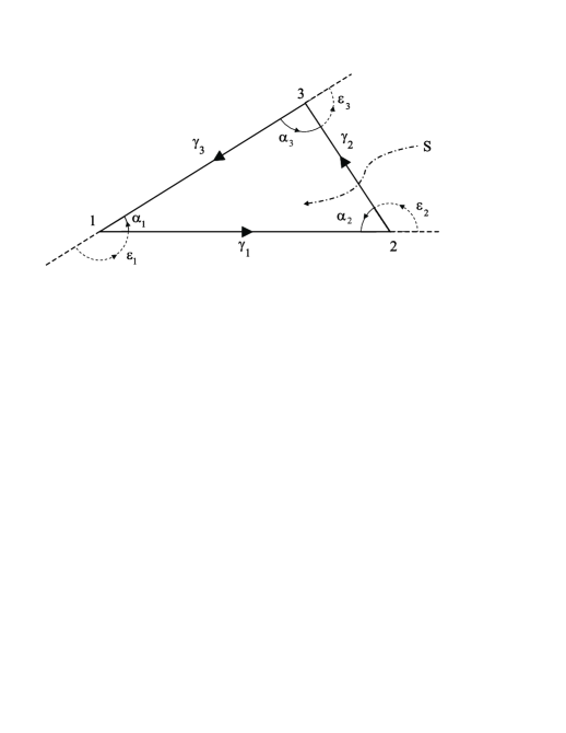
Figure 1: The way of counting angles in triangulation triangle.

We will prove that the sum of the internal angles $\alpha_{1},\alpha_{2},\alpha_{3}$ measured in a way shown in Fig. 1 fulfills the given Gauss relation:

$$\alpha_{1}+\alpha_{2}+\alpha_{3}-\pi=\int\limits_{S}{R_{12}},$$ (23)

where $\gamma_{1},\gamma_{2},\gamma_{3}$ are the geodesics shown in Fig. 1, $R_{12}$ is the two-form of a curvature, $S$ is the face which edge (boundary) is broken line $\gamma_{1}\cup\gamma_{2}\cup\gamma_{3}$. Namely if $\gamma$ is geodesics then a vector field $X$ tangent to it fulfills the equation $D_{X}X=0$. At every point of a geodesics one can introduce the orthonormal moving frame $e_{1},e_{2}$ and define an angle $\theta$ between vectors $e_{1}$ and $X$ what is shown in Fig. 2.

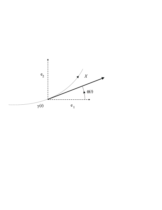
Figure 2: Definition of an angle $\theta$ (t is a parameter on a geodesics).

Then $X(t)=e_{1}\cos\theta(t)+e_{2}\sin\theta(t)$. Because $D_{X}X=0$ so

$$e_{1}\sin\theta[\omega_{12}(X)-\frac{{d\theta}}{{dt}}]+e_{2}\cos\theta[\frac{{d\theta}}{{dt}}-\omega_{12}(X)]=0.$$

i.e. $\frac{{d\theta}}{{dt}}(t)=\omega_{12}(X)$ where $\omega_{12}(X)=\left({e_{1},D_{X}e_{2}}\right)$ and $\omega_{12}=\left({e_{1},De_{2}}\right)$ is connection one form on manifold $M^{2}$. To get the Gauss relation Let us consider an integral

$$\oint\limits_{\gamma_{1}\cup\gamma_{2}\cup\gamma_{3}}{d\theta} = [\theta_{2}(in)-\theta_{1}(out)]+[\theta_{3}(in)-\theta_{2}(out)]+[\theta_{1}(in)-\theta_{3}(out)]$$

$$= [\theta_{1}(in)-\theta_{1}(out)]+[\theta_{2}(in)-\theta_{2}(out)]+[\theta_{3}(in)-\theta_{3}(out)]$$

$$= \psi_{1}+\psi_{2}+\psi_{3},$$

where $\psi_{i}=\theta_{i}(in)-\theta_{i}(out)$ for $i=1,2,3.$

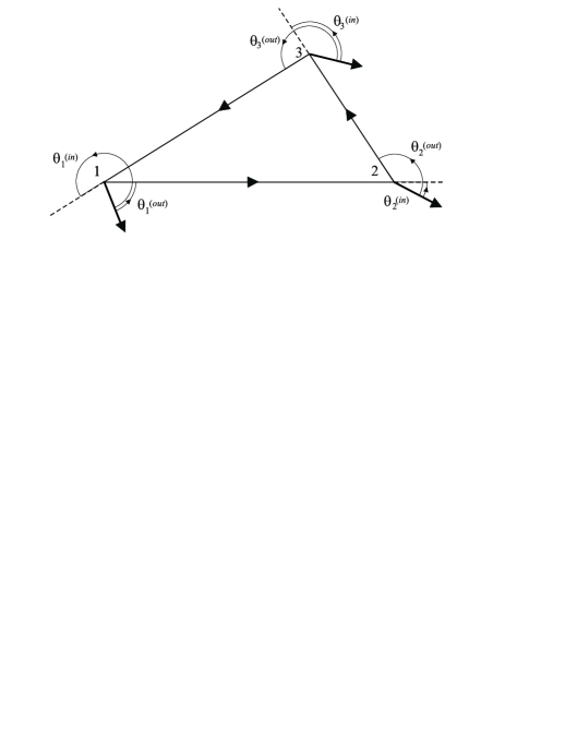
Figure 3: Way of counting angles in the geodesics triangle.

From Fig. 3 and Fig. 1 we can see that: $\psi_{1}=2\pi-\in_{1}$,$\psi_{2}=-\in_{2},$ $\psi_{3}=-\in_{3}$ and $\in_{i}+\alpha_{i}=\pi$ for $i=1,2,3$ - so $\psi_{1}=\pi+\alpha_{1}$, $\psi_{2}=\alpha_{2}-\pi$, $\psi_{3}=\alpha_{3}-\pi$ and hence:

$$\oint\limits_{\gamma_{1}\cup\gamma_{2}\cup\gamma_{3}}{d\theta=\alpha_{1}}+\alpha_{2}+\alpha_{3}-\pi=\oint\limits_{\gamma_{1}\cup\gamma_{2}\cup\gamma_{3}}{\omega_{12}}=\int\limits_{S}{d\omega_{12}}=\int\limits_{S}{R_{12}}.$$

Triangulation defines the sequence of the geodesics triangles $S_{1},S_{2},\ldots,S_{F}$, where $F$ is a number of faces. If with $(\alpha_{1}^{i},\alpha_{2}^{i},\alpha_{3}^{i})$ we will denote the interior angles in i - th geodesics triangle then

$$\sum\limits_{i=1}^{F}{\left({\alpha_{1}^{i}+\alpha_{2}^{i}+\alpha_{3}^{i}-\pi}\right)}=\sum\limits_{i=1}^{F}{\int\limits_{S_{i}}{R_{12}}}=\int\limits_{M^{2}}{R_{12}}=2\pi V-\pi F.$$

From relation $3F=2E$ we have $F=2\left({E-F}\right)$ so $\int\limits_{M^{2}}{R{}_{12}}=2\pi(F-E+V)$ or equivalently:

$$F-E+V\equiv\chi\left({M^{2}}\right)=\frac{1}{{2\pi}}\int\limits_{M^{2}}{R_{12}}.$$

The integer number $\chi(M^{2})$ is called the Euler characteristics of manifold $M^{2}$. The determined relation between the Euler characteristics of manifold $M^{2}$ and an integral of curvature two-form $R_{12}$ over this manifold we call the Gauss-Bonnet theorem. The Euler characteristic of manifolds is an intrinsic property of manifolds, and does not depend either on how we choose to triangulate $M^{2}$, or on how we choose the connection forms $\omega_{12}$. Moreover it can bee shown that two compact and closed surfaces $M_{1}$, $M_{2}$ are homeomorphic iff these surfaces are orientable (or not) and when their Euler characteristics are equal. This is a very important theorem about topological classification of the two dimensional surfaces. Any compact orientable closed surface is homeomorphic with connected sum of some number g of the tori $T^{2}$ and a sphere $S^{2}$ : $M^{2}\cong S^{2}\#T^{2}\#\ldots\#T^{2}$ We say that such a surface that it has a genus g and then its Euler characteristics is $2-2g$. The connected sum $M_{1}M_{2}$ of manifold $M_{1}$ and $M_{2}$ we construct as follows: a) we cut out the little ball in each manifold, b) we glue this manifolds along the edges of the mentioned above balls. Its easy to see that $\chi(M_{1}\#M_{2})=\chi(M_{1})+\chi(M_{2})-2$.

6.2 Vector field index on manifolds and Poincaré theorem

Theorem: Let $M^{2}$ be a closed, compact and orientable manifold:, let $V$ be the smooth vector field on $M^{2}$, let $p_{1},\ldots p_{R}$ be the isolated points at which the field $V$ takes zero value and $Ind_{p_{i}}V$ be the mean mean index of the vector field $V$ at point $p_{i}$. Then

$$\sum\limits_{i=1}^{R}{Ind_{p_{i}}}V=\frac{1}{{2\pi}}\int\limits_{M^{2}}{R_{12}}=\chi(M^{2}).$$

Proof:
Let $p_{i}$ be one of the points where the vector field $V$ takes value zero. In the neighborhood of this point exists the orthonormal moving frame $e_{1},e_{2}$. Besides everywhere (locally) outside the points $p_{1},p_{2},\ldots,p_{R}$ we can define another orthonormal moving frame $\hat{e}_{1},\hat{e}_{2}$ such that $\hat{e}_{1}=\frac{V}{{\left|V\right|}}$ and $\hat{e}_{2}$ is the unit vector orthogonal to $\hat{e}_{1}$. When at every point of manifold $M^{2}$ in which both moving frame are defined, the matrix of passage from one to the other is an element of orthogonal group with the determinant equal with $+1$. So

$$\left({e_{1},e_{2}}\right)=\left({\hat{e}_{1},\hat{e}_{2}}\right)\left[{\begin{array}[]{*{20}c}{\cos\alpha}&{-\sin\alpha}\\ {\sin\alpha}&{\cos\alpha}\\ \end{array}}\right].$$

The forms of the metric connection with respect to the moving frames $(e_{1},e_{2})$ and $\left({\hat{e}_{1},\hat{e}_{2}}\right)$ we define as: $De_{1}=e_{2}\otimes\omega_{21}$, $D\hat{e}_{1}=\hat{e}_{2}\otimes\hat{\omega}_{21}$. From the formula (10) results that:

$$Ind_{p_{i}}V=\frac{1}{{2\pi}}\oint\limits_{C}{[(\hat{e}_{1},e_{1}})d(\hat{e}_{1},e_{2})-(\hat{e}_{1},e_{2})d(\hat{e}_{1},e_{1})],$$ (25)

where $C$ is a curve closed encircling point $p_{i}$. We can calculate directly that:

$$(\hat{e}_{1},e_{1})d(\hat{e}_{1},e_{2})-(\hat{e}_{1},e_{2})d(\hat{e}_{1},e_{1})=d\alpha=\omega_{12}-\hat{\omega}_{12}.$$ (26)

Because $dd\alpha=0$ so $d\omega_{12}=d\hat{\omega}_{12}=R_{12}$. Hence:

$$Ind_{p_{i}}V=\frac{1}{{2\pi}}\oint\limits_{C}{d\alpha=\frac{1}{{2\pi}}}\oint\limits_{C}{[\omega_{12}}-\hat{\omega}_{12}].$$

To determine the sum of indices of the vector field $V$ connected with all points in which this fields takes the zero value, we must show that the surface $M^{2}$ is of the form $M^{2}=M_{+}\cup M_{-}$, where $M_{+}$ is a subset in $M^{2}$ compounded of the neighborhoods of this points where the field $V$ takes the value of zero (each such neighborhood contains exactly one zero of the field $V$), $M_{-}$ is the complement of a set $M_{+}$ in $M^{2}$. Hence:

$$\sum\limits_{i=1}^{R}{Ind_{p_{i}}}V = \frac{1}{{2\pi}}\int\limits_{\partial M_{+}}{[\omega_{12}}-\hat{\omega}_{12}]$$

$$= \frac{1}{{2\pi}}\int\limits_{\partial M_{+}}{\omega_{12}}+\frac{1}{{2\pi}}\int\limits_{\partial M_{-}}{\hat{\omega}_{12}}=\frac{1}{{2\pi}}\left[\int\limits_{M_{+}}{d\omega_{12}}+\int\limits_{M_{-}}{d\hat{\omega}_{12}}\right]$$

$$= \frac{1}{{2\pi}}\int\limits_{M^{2}}{R_{12}}=\chi(M^{2}).$$

We can see then that the sum of indices of any smooth vector field defined on a manifold $M^{2}$ does not depend from the choice of this field. This is the topological characteristics of the manifold $M^{2}$.

The Hopf-Poincaré theorem is the truth for $n=2r$ dimensional closed and compact manifolds though its proof in the general cases is much more difficult than for the two-dimensional case. If $V$ is the smooth vector field on $n$-dimensional Riemann manifold $M^{n}$ with takes the value zero in an isolated point $p_{0}\in M^{n}$ so we can surround this point with some $(n-1)$-dimensional closed manifold $S$ to the inside of which belongs a point $p_{0}$. If $(\hat{e}_{1},\hat{e}_{2},\ldots,\hat{e}_{n})$ is the orthogonal moving frame defined in such neighborhood of a point $p_{0}$ which contains the submanifold $S$, then the index of the vector field $V$ in a point $p_{0}$ is given by a formula:

$$Ind_{p_{0}}V=\frac{1}{{vol(S^{n-1})(n-1)!}}\int\limits_{S}{\in^{a_{1}a_{2}\ldots a_{n}}}(e_{1},\hat{e}_{a_{1}})d(e_{1},\hat{e}_{a_{2}})\wedge\ldots\wedge d(e_{1},\hat{e}_{a_{n}}),$$

where $e_{1}=\frac{V}{{\sqrt{(V,V)}}}$.

The above definition does not depend either on how we choose the submanifold $S$ or on how we choose a moving frame $\left({\hat{e}_{1},\hat{e}_{2},\ldots,\hat{e}_{n}}\right)$. If a vector field $V$ vanishes at points $p_{1},p_{2},\ldots.p_{N}\in M^{2r}$ then we can show that:

$$\sum\limits_{i=1}^{N}{Ind_{p_{i}}}V=\int\limits_{M^{2r}}{e(R)}$$ (27)

where $\int\limits_{M^{2r}}{e(R)}$ is the Euler characteristics of a manifold $M^{2r}$ when $e(R)=\frac{1}{{(4\pi)^{r}r!}}\eta^{a_{1}b_{1}\ldots a_{r}b_{r}}R_{a_{1}b_{1}}\wedge\ldots\wedge R_{a_{r}b_{r}}$ is the Euler form of the manifold $M^{2r}$, $R_{ab}=\frac{1}{2}R_{ab\mu\nu}dx^{\mu}\wedge dx^{\nu}$ is curvature two-form and $\eta^{a_{1}b_{1}\ldots a_{r}b_{r}}=\frac{1}{{\sqrt{g}}}\in^{a_{1}b_{1}\ldots a_{r}b_{r}}$. The proof of his theorem is analogous to the proof of the Hopf-Poincaré theorem in two dimensions, and is left as a (tedious) exercise to the reader. So:

1. An integral $\int\limits_{M^{2r}}{e(R)}$ does not depend from a choice of a metric $g$ and is equal to an integral number.

2. A sum $\sum\limits_{i=1}^{N}{Ind_{p_{i}}}V$ takes the same value for any smooth vector field on $M^{2r}$ having a finite number of isolated zeros.

3. If an integral $\int\limits_{M^{2r}}{e(R)}$ is different from zero then $M^{2r}$ does not have a smooth vector field not having the zero points.

An integral $\int\limits_{M^{2r}}{e(R)}$ we call Euler characteristic of manifold $M^{2r}$ and we mark it with the symbol $\chi(M^{2r})$. For the compact manifold the vanishing of Euler characteristics is the sufficient condition for existence pseudoriemanian metric of signature 1. Let the manifold $M^{n}$ be equipped with Riemann metric (,). According to the assumption there exists on $M^{n}$ the smooth unit vectors field $n$. On $M^{n}$ we define the quadratic form:

$$\left({V-n(V,n)}\right)^{2}-\left({V,n}\right)^{2}$$

where $V$ is any vector field on $M^{n}$ , and $V^{2}=(V,V)$. Defined in this way quadratic form has a signature 1.

Euler characteristics can be interpreted as an obstruction for constructing a smooth field on $M^{2r}$ which nowhere takes the value of zero. Generalization of this observation led to the creation of so called theory of the characteristic classes.

7 Conclusions

In this paper we provided a pedagogical discussion of topological quantum numbers from the perspective of the degree of a smooth mapping between smooth manifolds. The effective use of differential forms allowed us to give a novel derivation of the index of a vector field.

This in turn allowed us to derive the topological quantum number characterizing e.g. monopole configurations in the Yang-Mills-Higgs theory with gauge group $SU(2)$. We also demonstrated the bijectivity between the elements of the $SU(2)$ gauge group and unit vector fields on $R^{4}$.

Then we presented an original, elementary proof of Gauss-Bonnet and Poincaré-Hopf theorems for compact, closed, oriented, two dimensional manifolds. Unlike in the traditional proofs we used effective language of differential forms and skilfully used the notion of the form of connection. The new ingredient in the proof of the Poincaré-Hopf theorem was the expression of an index of the vector field at a point by suitable scalar products. This line of proof (after a generalization to higher dimensions) creates a possibility of formulation a sufficient condition for the existence of a pseudo-Riemannian metric on compact manifolds without a boundary. Such a condition would be very useful in modern cosmology. Finally we discuss the Poincaré-Hopf theorem for any even dimensional compact orientable manifold without boundary.

Acknowledgements

M.S. acknowledges the support by the Marie Curie Actions Transfer of Knowledge project COCOS (contract MTKD-CT-2004-517186).

References

- [1] N. Manton, P. Sutcliffe, Topological Solitons, Cambridge University Press (2004); M. Nakahara Geometry, Topology and Physics Second Edition. IOP Publishing Ltd (2003); G. L. Naber Topology, Geometry, and Gauge Fields. Interactions Springer-Verlag New York (2000); E. Bick, F. D. Steffen (Eds.) Topology and Geometry in Physics, Springer-Verlag Berlin Heidelberg (2005).
- [2] R. Rajamaran, Solitons and Instantons, North-Holland (1987).
- [3] A. Linde, Particle Physics and Inflationary Cosmology, Harwood, Chur, Switzerland (1990).
- [4] V.A. Rubakov, Nucl. Phys. B 203, 311 (1982).
- [5] B. A. Dubrovin, A. T. Fomenko, S. P. Novikov, Modern Geometry, Method and Applications I - III, Springer-Verlag, New York (1984-1990); A. S. Schwarz, Topology for Physicists, Springer-Verlag, Berlin Heidelberg (1994); M. Postnikov, Lectures in Geometry. Semester III, Mir Publisher, Moscow (1989); Y. Choquet-Bruhat, C. Dewitt-Morette, M. Dillard-Bleick, Analysis, Manifolds and Physics, North-Holland, Amsterdam (1982).
-
[6]
T. Eguchi, P. B. Gilkey, A. J. Hanson, Gravitation, Gauge Theories and Differential Geometry,
Phys. Rep. 66, No 6 (1980) 213-393;
G. ’t Hooft, Monopoles, Instantons and Confinement, arXiv:hep-th
\0010225v1; F. Lenz, Topological Concept in Gauge Theories, arXiv:hep-th\0403286v1; Y. Shnir, Magnetic Monopoles, Springer-Verlag, Berlin Heidelberg (2005). - [7] N. Straumann, General Relativity and Relativistic Astrophysics, Springer-Verlag, Berlin Heidelberg New York Tokyo (1984); M. Berger, A Panoramic View of Riemannian Geometry, Springer-Verlag, Berlin Heidelberg New York (2002).