Light and heavy baryon masses:
the $1/N_{c}$ expansion and the quark model

Abstract

We establish a connection between the quark model and the $1/N_{c}$ expansion mass formulas used in the description of baryon resonances. We show that a remarkable compatibility exists between the two methods in the light and heavy baryon sectors. In particular, the band number used to classify baryons in the $1/N_{c}$ expansion is explained by the quark model and the mass formulas for both approaches are consistent.

1 Introduction

Since pioneering work [1] in the field, the standard approach for baryon spectroscopy is the constituent quark model. The Hamiltonian typically contains a spin independent part formed of the kinetic plus the confinement energies and a spin dependent part given by a hyperfine interaction. The quark model results are de facto model dependent; it is therefore very important to develop model independent methods that can help in alternatively understanding baryon spectroscopy and support (or not) quark model assumptions. Apart from promising lattice QCD calculations [2], large $N_{c}$ QCD, or alternatively the $1/N_{c}$ expansion, offers such a method. In 1974 ’t Hooft generalized QCD from SU(3) to an arbitrary number of colors SU($N_{c}$) [3] and suggested a perturbative expansion in $1/N_{c}$, applicable to all QCD regimes. Witten has then applied the approach to baryons [4] and this has led to a systematic and predictive $1/N_{c}$ expansion method to study static properties of baryons. The method is based on the discovery that, in the limit $N_{c}\rightarrow\infty$, QCD possesses an exact contracted SU(2$N_{f}$) symmetry [5] where $N_{f}$ is the number of flavors. This symmetry is approximate for finite $N_{c}$ so that corrections have to be added in powers of $1/N_{c}$. Notice that a baryon is a bound state of $N_{c}$ quarks in the large $N_{c}$ formalism.

The $1/N_{c}$ expansion has successfully been applied to ground state baryons, either light [6, 7] or heavy [8, 9]. Its applicability to excited states is a subject of current investigations. The classification scheme used in the $1/N_{c}$ expansion for excited states is based on the standard SU(6) classification as in a constituent quark model. Baryons are grouped into excitation bands $N=0$, 1, 2,…, each band containing at least one SU(6) multiplet, the band number $N$ being the total number of excitation quanta in a harmonic oscillator picture.

The purpose of the present paper is to show that there is a compatibility between the quark model and the $1/N_{c}$ expansion methods. It is organized as follows. We first give a summary of the $1/N_{c}$ expansion method in Sec. 2. Then we present a relativistic quark model in Sec. 3 and derive analytic mass formulas from its Hamiltonian in Sec. 4. The comparison between the quark model and the $1/N_{c}$ mass formulas is discussed in Sec. 5 and conclusions are drawn in Sec. 6. We point out that the results summarized hereafter have been previously presented in Refs. [10, 11] for the light baryons and [12] for the heavy baryons. This work aims at being a pedagogical overview of these last three references.

2 Baryons in large $N_{c}$ QCD

2.1 Light nonstrange quarks

We begin with a summary of the $1/N_{c}$ expansion in the case $N_{f}=2$, but the arguments are similar for any $N_{f}$. The contracted SU(2$N_{f}$) symmetry is here the group SU(4) which has 15 generators: The spin and isospin subgroup generators $S_{i}$ and $T_{a}$ and operators acting on both spin and isospin degrees of freedom denoted by $G_{ia}$ ($i,a=1,2,3$).

The SU(4) algebra is

$$[S_{i},T_{a}]=0,\quad[S_{i},G_{ja}]=i\varepsilon_{ijk}G_{ka},\quad[T_{a},G_{ib}]=i\varepsilon_{abc}G_{ic},$$

$$[S_{i},S_{j}]=i\varepsilon_{ijk}S_{k},\quad[T_{a},T_{b}]=i\varepsilon_{abc}T_{c},\quad[G_{ia},G_{jb}]=\frac{i}{4}\delta_{ij}\varepsilon_{abc}T_{c}+\frac{i}{4}\delta_{ab}\varepsilon_{ijk}S_{k}.$$ (1)

In the limit $N_{c}\rightarrow\infty$ one has $[G_{ia},G_{jb}]\rightarrow 0$ which implies the existence of a contracted algebra. These SU(4) generators form the building blocks of the mass operator, at least in the ground state band ($N=0$). For orbitally excited states the generators $\ell^{i}$ of SO(3), as well as the tensor operator $\ell^{(2)ij}$ also appear since the symmetry under consideration is extended to SU(4) $\otimes$ SO(3).

In the $1/N_{c}$ expansion the mass operator $M$ has general form

$$M=\sum_{i}c_{i}O_{i},$$ (2)

where the coefficients $c_{i}$ encode the QCD dynamics and have to be determined from a fit to the existing data, and where the operators $O_{i}$ are SU(4) $\otimes$ SO(3) scalars of the form

$$O_{i}=\frac{1}{N^{n-1}_{c}}O^{(k)}_{\ell}\cdot O^{(k)}_{SF}.$$ (3)

Here $O^{(k)}_{\ell}$ is a $k$-rank tensor in SO(3) and $O^{(k)}_{SF}$ a $k$-rank tensor in SU(2)-spin, but invariant in SU(2)-flavor. The lower index $i$ in the left hand side represents a specific combination. Each $n$-body operator is multiplied by an explicit factor of $1/N^{n-1}_{c}$ resulting from the power counting rules [4], where $n$ represents the minimum of gluon exchanges to generate the operator. For the ground state, one has $k$ = 0. For excited states the $k=2$ tensor is important. In practical applications, it is customary to include terms up to $1/N_{c}$ and drop higher order corrections of order $1/N_{c}^{2}$.

As an example, we show the operators used in the calculation of the masses of the $[{\bf 70},1^{-}]$ multiplet up to order $1/N_{c}$ included [13] (the sum over repeated indices is implicit)

$$O_{1}=N_{c}\,{\bm{1}}\negthinspace\negthinspace\negthinspace\negthinspace\negthinspace ~{}O_{2}=\frac{1}{N_{c}}\ell^{i}S^{i},~{}~{}~{}O_{3}=\frac{1}{N_{c}}T^{a}T^{a},~{}~{}~{}O_{4}=\frac{1}{N_{c}}S^{i}S^{i},$$ , (4)

$$O_{5} =\frac{15}{N_{c}^{2}}\ell^{(2)ij}G^{ia}G^{ja},~{}~{}~{}O_{6}=\frac{3}{N_{c}^{2}}\ell^{i}T^{a}G^{ia}.$$

Note that although $O_{5}$ and $O_{6}$ carry a factor of $1/N_{c}^{2}$ their matrix elements are of order $1/N_{c}$ because they contain the coherent operator $G^{ia}$ which brings an extra factor $N_{c}$. $O_{1}=N_{c}\,{\bm{1}}$ is the trivial operator, proportional to $N_{c}$ and the only one surviving when $N_{c}\rightarrow\infty$ [4]. The operators $O_{2}$ (spin-orbit), $O_{5}$ and $O_{6}$ are relevant for orbitally excited states only. All the SU(4) quadratic invariants $S^{i}S^{i}$, $T^{a}T^{a}$ and $G^{ia}G^{ia}$ should enter the mass formula but they are related to each other by the operator identity [7]

$$\left\{S^{i},S^{i}\right\}+\left\{T^{a},T^{a}\right\}+4\left\{G^{ia},G^{ia}\right\}=\frac{1}{2}N_{c}(3N_{c}+4),$$ (5)

so one can express $G^{ia}G^{ia}$ in terms of $S^{i}S^{i}$ and $T^{a}T^{a}$.

Assuming an exact SU(2)-flavor symmetry, the mass formula for the ground state band up to order $1/N_{c}$ takes the following simple form [7]

$$M=c_{1}N_{c}+c_{4}\frac{1}{N_{c}}S^{2}+\mathcal{O}\left(\frac{1}{N_{c}^{3}}\right),$$ (6)

which means that for $N=0$ only the operators $O_{1}$ and $O_{4}$ (spin-spin) contribute to the mass.

Among the excited states, those belonging to the $N=1$ band, or equivalently to the $[{\bf 70},1^{-}]$ multiplet, have been most extensively studied, either for $N_{f}=2$ (see e.g. Refs. [14, 15, 16, 17, 18]) or for $N_{f}=3$ [19]. The $N=2$ band contains the $[{\bf 56^{\prime}},0^{+}]$, $[{\bf 56},2^{+}]$, $[{\bf 70},\ell^{+}]$ ($\ell$ = 0, 2), and $[{\bf 20},1^{+}]$ multiplets. There are no physical resonances associated to $[{\bf 20},1^{+}]$. The few studies related to the $N=2$ band concern the $[{\bf 56^{\prime}},0^{+}]$ for $N_{f}$ = 2 [20], $[{\bf 56},2^{+}]$ for $N_{f}=3$ [21], and $[{\bf 70},\ell^{+}]$ for $N_{f}=2$ [22], later extended to $N_{f}=3$ [23]. The method has also been applied [24] to highly excited non-strange and strange baryons belonging to $[{\bf 56},4^{+}]$, the lowest multiplet of the $N=4$ band [25].

The group theoretical similarity of excited symmetric states and the ground state makes the analysis of these states simple [21, 24]. For mixed symmetric states, the situation is more complex. There is a standard procedure which reduces the study of mixed symmetric states to that of symmetric states. This is achieved by the decoupling of the baryon into an excited quark and a symmetric core of $N_{c}-1$ quarks. This procedure has been applied to the $[{\bf 70},1^{-}]$ multiplet [14, 15, 16, 17, 18, 19] and to the $[{\bf 70},\ell^{+}]$ ($\ell$ = 0, 2) multiplets [22, 23]. But it has recently been shown that the decoupling is not necessary [13], provided one knows the matrix elements of the SU(2$N_{f}$) generators between mixed symmetric states. The derivation of these matrix elements is not trivial. For SU(4) they have been derived by Hecht and Pang [26] in the context of nuclear physics and adapted to quark physics in Ref. [13], where it has been shown that the isospin-isospin term becomes as dominant in $\Delta$ as the spin-spin term in $N$ resonances.

The derivation of SU(6) matrix elements between mixed symmetric states $[N_{c}-1,1]$ is underway [27].

A detailed description of the problems raised by the standard procedure [17] of the separation of a system of mixed spin-flavour symmetry $[N_{c}-1,1]$ into a symmetric core of $N_{c}-1$ quarks and an excited quark has been given in Refs. [28, 29].

2.2 Inclusion of strangeness

For light strange baryons ($N_{f}=3$) the mass operator in the $1/N_{c}$ expansion has the general form

$$M=\sum_{i=1}c_{i}O_{i}+\sum_{i=1}d_{i}B_{i},$$ (7)

where the operators $O_{i}$ are invariants under SU(6) transformations and the operators $B_{i}$ explicitly break SU(3)-flavor symmetry. In the case of nonstrange baryons, only the operators $O_{i}$ contribute, see Eq. (2). Therefore $B_{i}$ are defined such as their expectation values are zero for nonstrange baryons. The coefficients $d_{i}$ are determined from the experimental data including strange baryons. In Eq. (7) the sum over $i$ is finite and in practice it containes the most dominant operators. Examples of $O_{i}$ and $B_{i}$ can be found in Refs. [21, 23, 24].

Assuming that each strange quark brings the same contribution $\Delta M_{s}$ to the SU(3)-flavor breaking terms in the mass formula, we define the total contribution of strange quarks as [11]

$$n_{s}~{}\Delta M_{s}=\sum_{i=1}d_{i}B_{i},$$ (8)

where $n_{s}=-{\cal S}$ is the number of strange quarks in a baryon, ${\cal S}$ being its strangeness.

2.3 Heavy quarks

The approximate spin-flavor symmetry for large $N_{c}$ baryons containing light $q=\{u,d,s\}$ and heavy $Q=\{c,b\}$ quarks is SU(6)$\times$ SU(2)_c $\times$ SU(2)_b, i.e. there is a separate spin symmetry for each heavy flavor. Over a decade ago the $1/N_{c}$ expansion has been generalized to include an expansion in $1/m_{Q}$ and light quark flavor symmetry breaking [8]. The majority of the currently available experimental data concerning heavy baryons is related to ground state baryons made of one heavy and two light quarks [30]. Such heavy baryons, denoted as $qqQ$ baryons, have been recently reanalyzed within the combined $1/N_{c}$ and $1/m_{Q}$ expansion [9], and masses in good agreement with experiment have been obtained. A first attempt to extend this framework to excited heavy baryons can be found in Refs. [31] but much work remains to be done in this field. That is why we focus here on the $N=0$ band for $qqQ$ baryons only.

Let us first consider that SU(3)-flavor symmetry is exact. In this case the mass operator $M^{(1)}$ is a flavor singlet and in the combined $1/m_{Q}$ and $1/N_{c}$ expansion to order $1/m_{Q}^{2}$ it takes the following form

$$M^{(1)}=m_{Q}{\bm{1}}+\Lambda_{qq}+\lambda_{Q}+\lambda_{qqQ}.$$ (9)

The leading order term is $m_{Q}$ at all orders in the $1/N_{c}$ expansion. Next we have

$$\Lambda_{qq}=c_{0}\,N_{c}\,{\bm{1}}+\frac{c_{2}}{N_{c}}\,J^{2}_{qq},\quad{\rm and}\quad\lambda_{Q}=N_{Q}\frac{1}{2m_{Q}}\left(c^{{}^{\prime}}_{0}\,{\bm{1}}+\frac{c^{{}^{\prime}}_{2}}{N^{2}_{c}}J^{2}_{qq}\right),$$ (10)

where $\vec{J}_{qq}$ is identical to the total spin $\vec{S}_{qq}$ of the light quark pair when one deals with the $N=0$ band. Note that $\Lambda_{qq}$ contains the dynamical contribution of the light quarks and is independent of $m_{Q}$ while $\lambda_{Q}$ gives $1/m_{Q}$ corrections. The last term, $\lambda_{qqQ}$, contains the heavy-quark spin-symmetry violating operator which reads

$$\lambda_{qqQ}=2\frac{c^{{}^{\prime\prime}}_{2}}{N_{c}m_{Q}}\vec{J}_{qq}\cdot\vec{J}_{Q},$$ (11)

where $\vec{J}_{Q}$ is identical to the spin $\vec{S}_{Q}$ of the heavy quark.

The unknown coefficients $c_{0}$, $c_{2}$, $c^{{}^{\prime}}_{0}$, $c^{{}^{\prime}}_{2}$, and $c^{{}^{\prime\prime}}_{2}$ are functions of $1/N_{c}$ and of a QCD scale parameter $\Lambda$. Each coefficient has an expansion in $1/N_{c}$ where the leading term (in dimensionless units) is of order unity and does not depend on $1/m_{Q}$. Thus, without loss of generality, by including dimensions, one can set $c_{0}\equiv\Lambda$. The quantity $\Lambda$, as well as the other coefficients, have to be fitted to the available experimental data. In agreement with Ref. [8], we take

$$c_{0}=\Lambda,\quad c_{2}\sim\Lambda,\quad\quad c^{{}^{\prime}}_{0}\sim c^{{}^{\prime}}_{2}\sim c^{{}^{\prime\prime}}_{2}\sim{\Lambda}^{2}.$$ (12)

The inclusion of SU(3)-flavor breaking leads to an expansion of the mass operator in the SU(3)-violating parameter $\epsilon$ which contains the singlet $M^{(1)}$, an octet $M^{(8)}$, and a 27-plet $M^{(27)}$. The last term brings contributions proportional to $\epsilon^{2}$ and we neglect it. For $M^{(8)}$ we retain its dominant contribution $T^{8}$ to order $N^{0}_{c}$. Then the mass formula becomes

$$M=M^{(1)}+\epsilon T^{8}.$$ (13)

The flavor breaking parameter $\epsilon$ is governed by the mass difference $m_{s}-m$ (where $m$ is the average of the $m_{u}$ and $m_{d}$ masses) and therefore is $\epsilon\sim 0.2$-0.3. It is measured in units of the chiral symmetry breaking scale parameter $\Lambda_{\chi}\sim 1$ GeV.

3 Quark model for baryons

3.1 Main Hamiltonian

The quark model used here to describe baryons aims at capturing the main physical features of a three-quark system while keeping the formalism as simple as possible in order to get analytical mass formulas. It contains: Relativistic kinetic energy for the quarks, $Y$-junction confining potential, one-gluon exchange potential and quark self-energy contribution added as perturbative terms. Let us now shortly describe all these ingredients.

A baryon, seen as a bound state of three valence quarks, can be described, at the dominant order, by the spinless Salpeter Hamiltonian $H=\sum^{3}_{i=1}\sqrt{\vec{p}^{\,2}_{i}+m^{2}_{i}}+V_{Y}$, where $m_{i}$ is the bare mass of the quark $i$ and where $V_{Y}$ is the confining interaction potential. We use the bare mass of the quarks in the relativistic kinetic energy term as suggested by the field correlator method [32], but other approaches, like Coulomb gauge QCD, rather favor a running constituent quark mass [33]. Although very interesting conceptually, the influence of this choice on the mass spectra should not be so dramatic than it could have been expected at the first glance: First, the bare and constituent heavy quark masses are nearly identical. Second, the constituent light quark masses quickly decrease at large momentum and become similar to the bare masses; a common limit is reached for the excited states. The situation is thus mainly different for low-lying $nnn$ baryons ($u$ and $d$ quarks are commonly denoted as $n$), where the bare mass $m_{n}$ can be set equal to 0, but where the constituent mass is about 300 MeV [33]. However, the strength of additional interactions like one-gluon exchange (see next section) can be tuned in both cases and lead to final mass spectra which are quite similar.

Both the flux tube model [34] and lattice QCD [35] support the Y-junction picture for the confining potential: A flux tube starts from each quark and the three tubes meet at the Torricelli (or Steiner or Fermat) point of the triangle formed by the three quarks, let us say the $ABC$ triangle. This point $T$, located at $\vec{x}_{T}$, minimizes the sum of the flux tube lengths and leads to the following confining potential $V_{Y}=a\sum^{3}_{i=1}\left|\vec{x}_{i}-\vec{x}_{T}\right|$, where the position of quark $i$ is denoted by $\vec{x}_{i}$ and where $a$ is the energy density of the flux tubes. If all the angles of $ABC$ are less than 120^o, then the Toricelli point is such that the angles $\widehat{ATB}$, $\widehat{BTC}$, and $\widehat{ATC}$ are all equal to 120^o. If the angle corresponding to an apex is greater than 120^o, the Toricelli point is precisely at this apex.

As $\vec{x}_{T}$ is a complicated three-body function, it is interesting to approximate the confining potential by a more tractable form. In the following, we shall use

$$H_{R} =\sum^{3}_{i=1}\sqrt{\vec{p}^{\,2}_{i}+m^{2}_{i}}+V_{R},$$ (14)

$$V_{R} =k\,a\sum^{3}_{i=1}\left|\vec{x}_{i}-\vec{R}\right|,$$ (15)

where $\vec{R}$ is the position of the center of mass and $k$ is a corrective factor [36]. The accuracy of the replacement (15) has been checked to be very satisfactory (better than 5%) in this last reference provided that the appropriate scaling factor is used: $k_{0}=0.952$ for $qqq$ baryons and $k_{1}=0.930$ for $qqQ$ baryons. For highly excited states, the contribution of the configurations in which the Toricelli point is located on one of the quarks becomes more and more important, and one could think that the center of mass approximation (15) is then wrong. But in such cases the angle made by the Toricelli point and the other two quarks is larger than $120^{\rm o}$ and the center of mass is consequently still close to the true Toricelli point. The approximation (15), although being less accurate for highly excited states, remains however relevant.

3.2 Perturbative terms

Besides the Hamiltonian (14), other contributions are necessary to reproduce the baryon masses. We shall add them as perturbations to the dominant Hamiltonian (14). The most widespread correction is a Coulomb interaction term of the form

$$\Delta H_{oge}=-\frac{2}{3}\sum_{i<j}\frac{\alpha_{S,ij}}{|\vec{x}_{i}-\vec{x}_{j}|},$$ (16)

arising from one-gluon exchange processes, where $\alpha_{S,ij}$ is the strong coupling constant between the quarks $i$ and $j$. Actually, one should deal with a running form $\alpha_{S}(r)$, but it would considerably increase the difficulty of the computations. Typically, we need two values: $\alpha_{0}=\alpha_{S,qq}$ for a $qq$ pair and $\alpha_{1}=\alpha_{S,qQ}$ for a $qQ$ pair, in the spirit of what has been done in a previous study describing mesons in the relativistic flux tube model [37]. There it was found that $\alpha_{1}/\alpha_{0}\approx 0.7$ describes rather well the experimental data of $q\bar{q}$ and $Q\bar{q}$ mesons.

Another perturbative contribution to the mass is the quark self-energy. This is due to the color magnetic moment of a quark propagating through the QCD vacuum. It adds a negative contribution to the hadron masses [38]. The quark self-energy contribution for a baryon is given by

$$\Delta H_{qse}=-\frac{fa}{2\pi}\sum_{i}\frac{\eta(m_{i}/\delta)}{\mu_{i}},$$ (17)

where $\mu_{i}$ is the kinetic energy of the quark $i$, that is $\mu_{i}=\left\langle\sqrt{\vec{p}^{\,2}_{i}+m^{2}_{i}}\right\rangle$, the average being computed with the wave function of the unperturbed spinless Salpeter Hamiltonian (14). The factors $f$ and $\delta$ have been computed in quenched and unquenched lattice QCD studies; it seems well established that $3\leq f\leq 4$ and ($1.0\leq\delta\leq 1.3$) GeV [39]. The function $\eta(\epsilon)$ is analytically known; we refer the reader to Ref. [38] for an explicit formula. It can accurately be fitted by

$$\eta(\epsilon) \approx 1-\beta\epsilon^{2} \quad\textrm{with}\quad\beta=2.85 \quad\textrm{for}\quad 0\leq\epsilon\leq 0.3,$$

$$\approx\frac{\gamma}{\epsilon^{2}} \quad\textrm{with}\quad\gamma=0.79 \quad\textrm{for}\quad 1.0\leq\epsilon\leq 6.0.$$ (18)

Let us note that the corrections depending on the parameter $\gamma$ appear at order $1/m_{Q}^{3}$ in the mass formula, so they are not considered in this work.

We finally point out that the quark model we developed in this section is spin independent. This neglect of the fermionic nature of the quarks is the reason why such a model is often called “semirelativistic”: The implicit covariance is preserved, but spin effects are absent. Spin dependent contributions (spin-spin, spin-orbit, etc.) typically come from relativistic corrections to the one-gluon exchange potential. It is useful to mention that in our formalism such potential terms between the quarks $i$ and $j$ should be of the form [32]

$$V_{ij}\propto(\mu_{i}\mu_{j})^{-1}.$$ (19)

4 Mass formulas

4.1 The auxiliary field method

The comparison between the quark model and large $N_{c}$ mass formulas would be more straightforward if we could obtain analytical expressions. To this aim, the auxiliary field method is used in order to transform the Hamiltonian (14) into an analytically solvable one [40]. With $\lambda=k\,a$, we obtain

$$H(\mu_{i},\nu_{j})=\sum^{3}_{j=1}\left[\frac{\vec{p}^{\,2}_{j}+m^{2}_{j}}{2\mu_{j}}+\frac{\mu_{j}}{2}\right]+\sum^{3}_{j=1}\left[\frac{\lambda^{2}(\vec{x}_{j}-\vec{R})^{2}}{2\nu_{j}}+\frac{\nu_{j}}{2}\right].$$ (20)

The auxiliary fields, denoted as $\mu_{i}$ and $\nu_{j}$, are operators, and $H(\mu_{i},\nu_{j})$ is equivalent to $H$ up to their elimination thanks to the constraints

$$\left.\delta_{\mu_{i}}H(\mu_{i},\nu_{j})\right|_{\mu_{i}=\hat{\mu}_{i}} =0\ \Rightarrow\ \hat{\mu}_{i}=\sqrt{\vec{p}^{\,2}_{i}+m^{2}_{i}},$$

$$\left.\delta_{\nu_{j}}H(\mu_{i},\nu_{j})\right|_{\nu_{j}=\hat{\nu}_{j}} =0\ \Rightarrow\ \hat{\nu}_{j}=\lambda|\vec{x}_{j}-\vec{R}|.$$ (21)

$\left\langle\hat{\mu}_{i}\right\rangle$ is the quark kinetic energy, and $\left\langle\hat{\nu}_{i}\right\rangle$ is the energy of one flux tube, the average being computed with the wave function of the unperturbed spinless Salpeter Hamiltonian (14). The equivalence relation between Hamiltonians (14) and (20) is $H(\hat{\mu}_{i},\hat{\nu}_{j})=H$.

Although the auxiliary fields are operators, the calculations are considerably simplified if one considers them as variational parameters. They have then to be eliminated by a minimization of the masses, and their extremal values $\mu_{i,0}$ and $\nu_{j,0}$ are logically close to $\left\langle\hat{\mu}_{i}\right\rangle$ and $\left\langle\hat{\nu}_{j}\right\rangle$ respectively [40]. This technique can give approximate results very close to the exact ones [41]. If the auxiliary fields are assumed to be real numbers, the Hamiltonian (20) reduces formally to a nonrelativistic three-body harmonic oscillator, for which analytical solutions can be found. A first step is to replace the quark coordinates $\vec{x}_{i}=\left\{\vec{x}_{1},\vec{x}_{2},\vec{x}_{3}\right\}$ by the Jacobi coordinates $\vec{x}^{\,{}^{\prime}}_{k}=\{\vec{R},\vec{\xi},\vec{\eta}\,\}$ defined as [42]

$$\vec{R}=(\mu_{1}\vec{x}_{1}+\mu_{2}\vec{x}_{2}+\mu_{3}\vec{x}_{3})/\mu_{t},\quad{\rm with}\quad\mu_{t}=\mu_{1}+\mu_{2}+\mu_{3},$$ (22)

and $\vec{\xi}\propto\vec{x}_{1}-\vec{x}_{2},\ \vec{\eta}\propto(\mu_{1}\vec{x}_{1}+\mu_{2}\vec{x}_{2})/(\mu_{1}+\mu_{2})-\vec{x}_{3}$.

In the case of two quarks with mass $m$ and another with mass $m_{3}$, the mass spectrum of the Hamiltonian (20) is given by ($\mu_{1}=\mu_{2}=\mu$, $\nu_{1}=\nu_{2}=\nu$ by symmetry)

$$M(\mu,\mu_{3},\nu,\nu_{3})=\omega_{\xi}(N_{\xi}+3/2)+\omega_{\eta}(N_{\eta}+3/2)+\mu+\nu+\frac{\mu_{3}+\nu_{3}}{2}+\frac{m^{2}}{\mu}+\frac{m^{2}_{3}}{2\mu_{3}},$$ (23)

$${\rm where}\quad\omega_{\xi}=\frac{\lambda}{\sqrt{\mu\nu}},\quad\omega_{\eta}=\frac{\lambda}{\sqrt{2\mu+\mu_{3}}}\sqrt{\frac{\mu_{3}}{\mu\nu}+\frac{2\mu}{\mu_{3}\nu_{3}}}.$$ (24)

The integers $N_{\xi/\eta}$ are given by $2n_{\xi/\eta}+\ell_{\xi/\eta}$, where $n_{\xi/\eta}$ and $\ell_{\xi/\eta}$ are the radial and orbital quantum numbers relative to the variable $\vec{\xi}/\vec{\eta}$ respectively. Moreover, $\left\langle\vec{\xi}^{\,2}\right\rangle$ and $\left\langle\vec{\eta}^{\,2}\right\rangle$ are analytically known. This eventually allows to compute $\left\langle(\vec{x}_{1}-\vec{x}_{3})^{2}\right\rangle$ and $\left\langle(\vec{x}_{2}-\vec{x}_{3})^{2}\right\rangle$, which are needed to know the one-gluon exchange contribution.

The four auxiliary fields appearing in the mass formula (23) have to be eliminated by solving simultaneously the four constraints

$$\partial_{\mu}M(\mu,\mu_{3},\nu,\nu_{3})=0, \quad\partial_{\mu_{3}}M(\mu,\mu_{3},\nu,\nu_{3})=0,$$

$$\partial_{\nu}M(\mu,\mu_{3},\nu,\nu_{3})=0, \quad\partial_{\nu_{3}}M(\mu,\mu_{3},\nu,\nu_{3})=0.$$ (25)

This task cannot be analytically performed in general, but solutions can fortunately be found in the case of light and heavy baryons.

4.2 Light baryons

Since we do not distinguish between the $u$ and $d$ quarks in our quark model and commonly denote them as $n$, there are only four possible configurations: $nnn$, $sss$, $nss$ and $snn$, that can all be described by the mass formula (23). Important simplifications occur by setting $m_{n}=0$, which is a good approximation of the $u$ and $d$ quark bare masses. However, the non vanishing value for $m_{s}$ causes Eqs. (4.1) to have no analytical solution unless a power expansion in $m_{s}$ is performed. This is justified a priori since the strange quark is still a light one. After such a power expansion, the final mass formula reads [10]

$$M_{qqq} =M_{0}+n_{s}\,\Delta M_{0s}\quad\quad(n_{s}=0,1,2,3),$$

$$M_{0} =6\mu_{0}-\frac{2k_{0}a\alpha_{0}}{\sqrt{3}\mu_{0}}-\frac{3fa}{2\pi\mu_{0}},\quad\Delta M_{0s}=\frac{m^{2}_{s}}{\mu_{0}}\left[\frac{1}{2}-\frac{k_{0}a\alpha_{0}}{6\sqrt{3}\mu_{0}^{2}}+\frac{fa}{2\pi}\left(\frac{3}{4\mu^{2}_{0}}+\frac{\beta}{\delta^{2}}\right)\right],$$

$$\mu_{0} =\sqrt{\frac{k_{0}a(N+3)}{3}}.$$ (26)

The mass formula $M_{qqq}$ depends only on $N=N_{\xi}+N_{\eta}$. The contribution of terms proportional to $N_{\xi}-N_{\eta}$, vanishing for $n_{s}=0$ and 3, was found to be very weak in the other cases by a numerical resolution of Eqs. (4.1).

An important feature of the above mass formula has to be stressed: It only depends on $N$ the total number of excitation quanta of the system. But, this integer is precisely the band number introduced in large $N_{c}$ QCD to classify the baryon states in a harmonic oscillator picture. Indeed the spinless Salpeter Hamiltonian (14) has been transformed into a harmonic oscillator by the auxiliary field method and it is thus natural that a such band number appears. The great advantage of the auxiliary field method is that it allows to obtain analytical mass formulas for a relativistic Hamiltonian while making explicitly the band number used in the large $N_{c}$ classification scheme to appear. The origin of $N$ is thus explained by the dynamics of the three-quark system and the comparison with the $1/N_{c}$ mass formulas is therefore possible.

4.3 Heavy baryons

A mass formula for $qqQ$ baryons can also be found from Eq. (23). An expansion in $m_{s}$ is still needed to get analytical expressions, but an expansion in $1/m_{Q}$ can also be done since we deal with one heavy quark. One obtains [12]

$$M_{qqQ} =m_{Q}+M_{1}+n_{s}\,\Delta M_{1s}+\Delta M_{Q}\quad\quad(n_{s}=0,1,2),$$

$$M_{1} =4\mu_{1}-\frac{2}{3}\left(\alpha_{0}\sqrt{\frac{k_{1}a}{2N_{\xi}+3}}+2\alpha_{1}\sqrt{\frac{2k_{1}a}{N+3}}\right)-\frac{fa}{\pi\mu_{1}},$$

$$\Delta M_{1s} =\frac{m_{s}^{2}}{\mu_{1}}\left[\frac{1}{2}-\frac{1}{12\mu_{1}}\left(\alpha_{0}\sqrt{\frac{k_{1}a}{2N_{\xi}+3}}+2\alpha_{1}\sqrt{\frac{2k_{1}a}{N+3}}\right)+\frac{fa}{2\pi}\left(\frac{3}{4\mu_{1}^{2}}+\frac{\beta}{\delta^{2}}\right)\right],$$

$$\Delta M_{Q} =\frac{k_{1}a}{2m_{Q}}\left[\left(1-\frac{fa}{2\pi\mu_{1}^{2}}\right)G(N,N_{\eta})-\frac{\alpha_{0}}{6}\sqrt{\frac{2N_{\eta}+3}{2N_{\xi}+3}}\left(\sqrt{\frac{2(2N_{\eta}+3)}{N+3}}-1\right)\right.$$

$$\phantom{=\frac{k_{1}a}{2m_{Q}}+}\left.+\frac{4\alpha_{1}}{3}\frac{2N_{\eta}+3}{N+3}\right],$$

$$\mu_{1} =\sqrt{\frac{k_{1}a(N+3)}{2}},\quad G(N,N_{\eta})=\sqrt{2N_{\eta}+3}\left(\sqrt{2(N+3)}-\sqrt{2N_{\eta}+3}\right).$$ (27)

At the lowest order in $m_{s}$ and $1/m_{Q}$, this mass formula depends only on $N$. However, when corrections are added, the mass formula is no longer symmetric in $N_{\eta}$ and $N_{\xi}$. Is it still possible to find a single quantum number? The answer is yes, provided we make the reasonable assumption that an excited heavy baryon will mainly “choose” the configuration that minimizes its mass.

The dominant correction of order $1/m_{Q}$ is the term that depends on the function $G(N,N_{\eta})$. The baryon mass is lowered when $G(N,N_{\eta})$ is minimal, that is to say for $N_{\eta}=N$. The analysis of the dominant part of the Coulomb term shows that the baryon mass is also lowered in this case. So it is natural to assume that the favored configuration, minimizing the baryon energy, is $N_{\eta}=N$ and $N_{\xi}=0$. It is also possible to reach the same conclusion by checking that an excitation of type $N_{\eta}$ will keep the baryon smaller in average than the corresponding excitation in $N_{\xi}$. This is favored because of the particular shape of the potential, having for consequence that the more the system is small, the more it is light.

As for light baryons, the quark model shows that heavy baryons can be labeled by a single band number $N$ in a harmonic oscillator picture. A light diquark-heavy quark structure is then favored since the light quark pair will tend to remain in its ground state. Note that the diquark picture combined with a detailed relativistic quark model of heavy baryons leads to mass spectra in very good agreement with the experimental data [43].

4.4 Regge trajectories

The band number $N$ emerges from the quark model as a good classification number for baryons. It is now interesting to focus on the behavior of the baryon masses at large values of $N$, i.e. for highly excited states. In this limit, the formula (4.2) gives

$$M^{2}_{qqq} \approx 12\,ak_{0}(N+3)-\frac{24}{\sqrt{3}}ak_{0}\alpha_{0}-\frac{16fak_{0}}{\pi}+6\left[1+\frac{fak_{0}\beta}{\pi\delta^{2}}\right]n_{s}m_{s}^{2}.$$ (28)

Our quark model thus states that light baryons should follow Regge trajectories, that is a linear relation $M^{2}\propto N$, with a common slope, irrespective of the strangeness of the baryons. The Regge slope of strange and nonstrange baryons is also predicted to be independent of the strangeness in the $1/N_{c}$ expansion method [44]. Too few experimental data are unfortunately available to check this result. In the heavy baryon sector, the mass formula (4.3) with $N_{\xi}=0$ and $N_{\eta}=N$ becomes at the dominant order

$$(M-m_{Q})^{2}=8a\frac{k_{1}}{k_{0}}(N+3).$$ (29)

This model predicts Regge trajectories for heavy baryons, with a slope of $8ak_{1}/k_{0}\approx 7.8a$ instead of $12ak_{0}\approx 11.4\,a$ for light baryons.

The Regge slope for light baryons is here given by $12ak_{0}$. However, from experiment we know that the Regge slopes for light baryons and light mesons are approximately equal. For light mesons, the exact value obtained in the framework of the flux tube model is $2\pi a$, a lower value than the one obtained from formula (28). This is due to the auxiliary field method that has been shown to overestimate the masses [45]. What can be it done to remove this problem is to rescale $a$. Let us define $\sigma$ such that $12ak_{0}=2\pi\sigma$; then the formula (28) is able to reproduce the light baryon Regge slope for a physical value $\sigma$ of the flux tube energy density. The scaling $a=\pi\sigma/(6k_{0})$ will consequently be assumed in the rest of this paper.

5 Large $N_{c}$ QCD versus Quark Model results

5.1 Light nonstrange baryons

The coefficients $c_{i}$ appearing in the $1/N_{c}$ mass operator can be obtained from a fit to experimental data. For example, the case $N=0$ is particularly simple. Equation (6) can be applied to $N$ and $\Delta$ baryons. Taking $N_{c}=3$ together with $M_{N}=940$ MeV for $S=1/2$, and $M_{\Delta}=1232$ MeV for $S=3/2$, we get

$$c_{1}^{(N=0)}=289~{}\mathrm{MeV},~{}~{}~{}~{}~{}c_{4}^{(N=0)}=292~{}\mathrm{MeV}.$$ (30)

Since the spin-orbit contribution vanishes for $N=0$, no information can be obtained for $c_{2}$. We refer the reader to Refs. [19, 21, 22, 24] for the determination of $c_{i}$ at $N>0$.

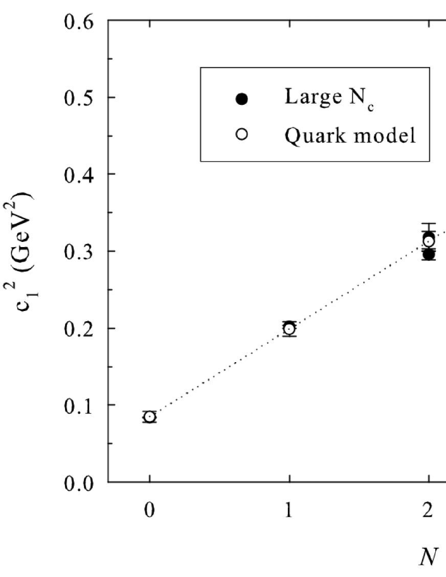
Figure 1: Plot of $c^{2}_{1}$ (left) and $\Delta M_{s}$ (right) versus the band number $N$. The values computed in the $1/N_{c}$ expansion (full circles) from a fit to experimental data are compared with the quark model results with $\sigma=0.163$ GeV², $\alpha_{0}=0.4$, $f=3.6$, and $m_{s}=0.240$ GeV (empty circles and dotted line to guide the eyes). No data is available for $N=3$ in large $N_{c}$ studies. The large $N_{c}$ data are nearly indistinguishable from the quark model prediction in the left plot.

In the $1/N_{c}$ expansion method, the dominant term $c_{1}\,N_{c}$ in the mass formula (2) contains the spin-independent contribution to the baryon mass, which in a quark model language represents the confinement and the kinetic energy. So, it is natural to identify this term with the mass given by the formula (4.2). Then, for $N_{c}=3$ we have

$$c^{2}_{1} = \frac{M^{2}_{qqq}}{9}=\frac{2\pi}{9}\sigma(N+3)-\frac{4\pi}{9\sqrt{3}}\,\sigma\alpha_{0}-\frac{f\sigma}{3}.$$ (31)

Figure 1 shows a comparison between the values of $c^{2}_{1}$ obtained in the $1/N_{c}$ expansion method and those derived from Eq. (31) for various values of $N$. From this comparison one can see that the results of large $N_{c}$ QCD are entirely compatible with the formula (31) provided $\sigma=0.163$ GeV², a rather low but still acceptable value according to usual potential models, $\alpha_{0}=0.4$, and $f=3.6$: These are very standard values.

Figure 2: Values of $c_{2}$ (left) and $c_{4}$ (right) versus the band number $N$. The values computed in the $1/N_{c}$ expansion (full circles) from a fit to experimental data are compared with results from formula (32) (empty circles and dotted line to guide the eyes). No data is available for $N=3$ in large $N_{c}$ studies.

Equation (19) implies that $c_{2}$ and $c_{4}\propto\mu^{-2}_{0}$. Therefore we expect the dependence of $N$ of these coefficients to be of the form

$$c_{2}=\frac{c^{0}_{2}}{N+3},\quad c_{4}=\frac{c^{0}_{4}}{N+3}.$$ (32)

We see that such a behavior is consistent with the large $N_{c}$ results in Fig. 2. We chose $c^{0}_{2}=208\pm 60$ MeV so that the point with $N=1$, for which the uncertainty is minimal, is exactly reproduced. Let us recall that the spin-orbit term is vanishing for $N=0$, so no large $N_{c}$ result is available in this case. To compute the parameter $c^{0}_{4}$ a fit was performed on all the large $N_{c}$ results. In this way we have obtained $c^{0}_{4}=1062\pm 198$ MeV. Note that $c^{0}_{4}\gg c^{0}_{2}$. This shows that the spin-spin contribution is much larger than the spin-orbit contribution, which justifies the neglect of the spin-orbit one in quark model studies.

5.2 Light strange baryons

We have first to find out the values of $\Delta M_{s}$ coming from the $1/N_{c}$ expansion. For $N=0$, 1, and 3, they can be found in Ref. [44], and the case $N=4$ is available in Ref. [24]. The situation is slightly more complicated in the $N=2$ band due to a larger number of available results. We refer the reader to Ref. [11] for a detailed discussion about the computation of $\Delta M_{s}$ in this case.

The mass shift due to strange quarks is given in the quark model formalism by $\Delta M_{0s}$ in Eq. (4.2). A comparison of this term with its large $N_{c}$ counterpart is given in Fig. 1, where we used the same parameters as for light nonstrange baryons. The only new parameter is the strange quark mass, that we set equal to $240$ MeV, a higher mass than the PDG value but rather common in quark model studies. One can see that the quark model predictions are always located within the error bars of the large $N_{c}$ results. Except for $N=3$, whose large $N_{c}$ value would actually require further investigations, the central values of $\Delta M_{s}$ in the large $N_{c}$ approach are close to the quark model results and they decrease slowly and monotonously with increasing $N$. Thus, in both approaches, one predicts a mass correction term due to SU(3)-flavor breaking which decreases with the excitation energy (or $N$).

5.3 Heavy baryons

As mentioned previously, our present study is restricted to ground state heavy baryons made of one heavy and two light quarks. In the $1/N_{c}$, $1/m_{Q}$ expansion the parameters to be fitted are $\Lambda$, $m_{Q}$ and $\epsilon\Lambda_{\chi}$. At the dominant order, the value of $\Lambda$ can be extracted from the mass combinations [8]

$$\Lambda_{Q}=m_{Q}+N_{c}\Lambda,\quad\frac{1}{3}(\Sigma_{Q}+2\Sigma^{*}_{Q})-\Lambda_{Q}=2\frac{\Lambda}{N_{c}},\quad\Sigma^{*}_{Q}-\Sigma_{Q}=\frac{3}{2}\left(\frac{2\Lambda^{2}}{N_{c}m_{Q}}\right),$$ (33)

resulting from the mass formula (9). Here and below the particle label represents its mass. A slightly more complicated mass combination, involving light baryons as well as heavy ones, directly leads to $m_{Q}$, that is [9]

$$\frac{1}{3}(\Lambda_{Q}+2\Xi_{Q})-\frac{1}{4}\left[\frac{5}{8}(2N+3\Sigma+\Lambda+2\Xi)-\frac{1}{10}(4\Delta+3\Sigma^{*}+2\Xi^{*}+\Omega)\right]=m_{Q}.$$ (34)

This mass combination gives

$$m_{c}=1315.1\pm 0.2~{}{\rm MeV},\quad m_{b}=4641.9\pm 2.1~{}{\rm MeV},$$ (35a)

while the value

$$\Lambda\approx 324~{}{\rm MeV}$$ (35b)

ensures that the mass combinations (33) are optimally compatible with the experimental values for $Q=c$ and $b$. A measure of the SU(3)-flavor breaking factor is given by [8]

$$\Xi_{Q}-\Lambda_{Q}=\frac{\sqrt{3}}{2}\,(\epsilon\Lambda_{\chi}).$$ (36)

The value $(\epsilon\Lambda_{\chi})=206$ MeV leads to $\Xi_{Q}-\Lambda_{Q}=178$ MeV, which is the average value of the corresponding experimental data.

The new parameters appearing in the quark model are $m_{c}$, $m_{b}$, $k_{1}=0.930$, and $\alpha_{1}$. For the other parameters we keep the values fitted in the light baryon sector. We take $\alpha_{1}=0.7\alpha_{0}$ from the quark model study of Ref. [37]. The heavy quark masses can be fitted to the experimental data as follows. The quark model mass formula (4.3) is spin independent; it should thus be suitable to reproduce the masses of heavy baryons for which $J^{2}_{qq}=0$. Namely, one expects that

$$\left.M_{nnc}\right|_{N=0}=\Lambda_{c}=2286.46\pm 0.14\ {\rm MeV},\quad\left.M_{nnb}\right|_{N=0}=\Lambda_{b}=5620.2\pm 1.6\ {\rm MeV}.$$ (37)

These values are reproduced by formula (4.3) with $m_{c}=1.252$ GeV and $m_{b}=4.612$ GeV. It is worth mentioning that we predict $\left.M_{nsc}\right|_{N=0}=2433$ MeV and $\left.M_{nsb}\right|_{N=0}=5767$ MeV with these parameters. These values are very close to the experimental $\Xi_{c}$ and $\Xi_{b}$ masses respectively.

We can now compare the quark model and the $1/N_{c}$, $1/m_{Q}$ mass formulas. On the one hand the mass combination (34) leads to $m_{c}=1315$ MeV and $m_{b}=4642$ MeV. On the other hand, the quark model mass formula (4.3) is compatible with the experimental data provided that $m_{c}=1252$ MeV and $m_{b}=4612$ MeV. Both approaches lead to quark masses that differ by less than 5%. Thus they agree at the dominant order, where only $m_{Q}$ is present.

The other parameter involved in the large $N_{c}$ mass formula is $\Lambda$. A comparison of the spin independent part of the mass formulas (9) and (4.3) leads to the following identification for $N_{c}=3$

$${c_{0}}=\frac{1}{3}\left.M_{1}\right|_{N=0}=\frac{4}{3}\mu_{1}-\frac{2}{27}\sqrt{\frac{k_{1}\pi\sigma}{2k_{0}}}(\alpha_{0}+2\sqrt{2}\alpha_{1})-\frac{f\sigma}{18k_{0}\mu_{1}},\ {\rm with}\ \mu_{1}=\sqrt{k_{1}\pi\sigma/4k_{0}}.$$ (38)

According to Eqs. (12) and (35b) one has $c_{0}=\Lambda\simeq 0.324$ GeV. The quark model gives 0.333 GeV for the expression after the second equality sign in Eq. (38), which means a very good agreement for the QCD scale $\Lambda$. The terms of order $1/m_{Q}$ lead to the identity

$$c^{{}^{\prime}}_{0}=2m_{Q}\left.\Delta M_{Q}\right|_{N=0}=\frac{k_{1}\pi\sigma}{6k_{0}}\left[3\left(\sqrt{2}-1\right)\left(1-\frac{f\sigma}{12k_{0}\mu_{1}^{2}}\right)-\frac{\alpha_{0}}{6}\left(\sqrt{2}-1\right)+\frac{4\alpha_{1}}{3}\right].$$ (39)

Note that to test this relation the value of $m_{Q}$ is not needed, like for the identity (38). The large $N_{c}$ parameter, $\Lambda=0.324$ GeV, gives for the left hand side of (39) $c^{{}^{\prime}}_{0}\sim\Lambda^{2}=0.096$ GeV² and the quark model gives for the right hand side 0.091 GeV², which is again a good agreement. Finally, the SU(3)-flavor breaking term is proportional to $\epsilon\Lambda_{\chi}\sim m_{s}-m\sim m_{s}$ in the mass formula (13). Equations (13), (4.3), and (36) lead to

$$\frac{\sqrt{3}}{2}\epsilon\Lambda_{\chi}=\left.\Delta M_{1s}\right|_{N=0}=\frac{m_{s}^{2}}{\mu_{1}}\left[\frac{1}{2}-\frac{1}{36\mu_{1}}\sqrt{\frac{k_{1}\pi\sigma}{2k_{0}}}\left(\alpha_{0}+2\sqrt{2}\alpha_{1}\right)+\frac{f\sigma}{12k_{0}}\left(\frac{3}{4\mu_{1}^{2}}+\frac{\beta}{\delta^{2}}\right)\right].$$ (40)

The large $N_{c}$ value $\epsilon\Lambda_{\chi}=0.206$ GeV and the quark model estimate $0.170$ GeV also compare satisfactorily. We point out that, except for $m_{c}$ and $m_{b}$, all the model parameters are determined from theoretical arguments combined with phenomenology, or are fitted on light baryon masses. The comparison of our results with the $1/N_{c}$ expansion coefficients $c_{0}$, $c^{{}^{\prime}}_{0}$ and $\epsilon\Lambda_{\chi}$ are independent of the $m_{Q}$ values. So we can say that this analysis is parameter free.

An evaluation of the coefficients $c_{2}$, $c_{2}^{\prime}$, and $c_{2}^{\prime\prime}$ through a computation of the spin dependent effects is out of the scope of the present approach. But at the dominant order, one expects from Eq. (19) that $c_{2}\propto\mu^{-2}_{1}$ and $c_{2}^{\prime\prime}\propto\mu^{-1}_{1}$. The ratio $c_{2}^{\prime\prime}/c_{2}$ should thus be of order $\mu_{1}=356$ MeV, which is roughly in agreement with Eq. (12) stating that $c_{2}^{\prime\prime}/c_{2}\sim\Lambda$. This gives an indication that the quark model and the $1/N_{c}$ expansion method would remain compatible if the spin-dependent effects were included.

6 Conclusions

We have established a connection between the quark model and the $1/N_{c}$ expansion both for light baryons and for heavy baryons containing a heavy quark. In the latter case the $1/N_{c}$ expansion is supplemented by an $1/m_{Q}$ expansion due to the heavy quark. A clear correspondence between the various terms appearing in the $1/N_{c}$ and quark model mass formulas is observed, and the fitted coefficients of the $1/N_{c}$ mass formulas can be quantitatively reproduced by the quark model.

These results bring reliable QCD-based support in favor of the constituent quark model assumptions and lead to a better insight into the coefficients $c_{i}$ encoding the QCD dynamics in the $1/N_{c}$ mass operator. In particular, the dynamical origin of the band number labeling the baryons in large $N_{c}$ QCD is explained by the quark model.

As an outlook, we mention two important studies that we hope to make in the future. First, the $N=1$ baryons of $qqQ$ type are poorly known in the $1/N_{c}$, $1/m_{Q}$ expansion. They should be reconsidered and compared to the quark model. Second, the ground state baryons made of two heavy quarks and a light quark could be studied in a combined $1/N_{c}$, $1/m_{Q}$ expansion-quark model approach, leading to predictions for the mass spectrum of these baryons.

References

- [1] N. Isgur and G. Karl, Phys. Rev. D 18, 4187 (1978); Phys. Rev. D 19, 2653 (1979); Phys. Rev. D 20, 1191 (1979).
- [2] S. Aoki et al. [PACS-CS Collaboration], arXiv:0807.1661 [hep-lat].
- [3] G. ’t Hooft, Nucl. Phys. 72, 461 (1974).
- [4] E. Witten, Nucl. Phys. B 160, 57 (1979).
- [5] J. L. Gervais and B. Sakita, Phys. Rev. Lett. 52, 87 (1984); Phys. Rev. D 30, 1795 (1984); R. Dashen and A. V. Manohar, Phys. Lett. B 315, 425 (1993); 438 (1993).
- [6] R. Dashen, E. Jenkins, and A. V. Manohar, Phys. Rev. D 49, 4713 (1994); 51, 2489 (1995);51, 3697 (1995).
- [7] E. Jenkins, Ann. Rev. Nucl. Part. Sci. 48, 81 (1998).
- [8] E. E. Jenkins, Phys. Rev. D 54, 4515 (1996).
- [9] E. E. Jenkins, Phys. Rev. D 77, 034012 (2008).
- [10] C. Semay, F. Buisseret, N. Matagne, and Fl. Stancu, Phys. Rev. D 75, 096001 (2007).
- [11] C. Semay, F. Buisseret, and Fl. Stancu, Phys. Rev. D 76, 116005 (2007).
- [12] C. Semay, F. Buisseret, and Fl. Stancu, Phys. Rev. D 78, 076003 (2008).
- [13] N. Matagne and F. Stancu, Nucl. Phys. A 811, 291 (2008).
- [14] C. D. Carone et al., Phys. Rev. D 50, 5793 (1994).
- [15] J. L. Goity, Phys. Lett. B 414, 140 (1997).
- [16] D. Pirjol and T. M. Yan, Phys. Rev. D 57, 1449 (1998) ; 57, 5434 (1998).
- [17] C. E. Carlson, C. D. Carone, J. L. Goity, and R. F. Lebed, Phys. Lett. B 438, 327 (1998); Phys. Rev. D 59, 114008 (1999).
- [18] T. D. Cohen and R. F. Lebed, Phys. Rev. D 67, 096008 (2003).
- [19] C. L. Schat, J. L. Goity, and N. N. Scoccola, Phys. Rev. Lett. 88, 102002 (2002);J. L. Goity, C. L. Schat, and N. N. Scoccola, Phys. Rev. D 66, 114014 (2002).
- [20] C. E. Carlson and C. D. Carone, Phys. Lett. B 484, 260 (2000).
- [21] J. L. Goity, C. L. Schat, and N. N. Scoccola, Phys. Lett. B 564, 83 (2003).
- [22] N. Matagne and Fl. Stancu, Phys. Lett. B 631, 7 (2005).
- [23] N. Matagne and Fl. Stancu, Phys. Rev. D 74, 034014 (2006).
- [24] N. Matagne and Fl. Stancu, Phys. Rev. D 71, 014010 (2005).
- [25] P. Stassart and Fl. Stancu, Z. Phys. A 359, 321 (1997).
- [26] K. T. Hecht and S. C. Pang, J. Math. Phys. 10 (1969) 1571.
- [27] N. Matagne and Fl. Stancu, in preparation.
- [28] N. Matagne and Fl. Stancu, Phys. Rev. D 77, 054026 (2008)
- [29] N. Matagne and Fl. Stancu, AIP Conf. Proc. 1038, 278 (2008), arXiv:0805.4368 [hep-ph].
- [30] C. Amsler et al. [Particle Data Group], Phys. Lett. B 667, 1 (2008).
- [31] J.-P. Lee, C. Liu, and H. S. Song, Phys. Rev. D 59, 034002 (1998); 62, 096001 (2000).
- [32] Yu. A. Simonov, hep-ph/9911237; A. Yu. Dubin, A. B. Kaidalov, and Yu. A. Simonov, Phys. Atom. Nucl 56, 1745 (1993).
- [33] F. J. Llanes-Estrada and S. R. Cotanch, Phys. Rev. Lett. 84, 1102 (2000); Phys. Lett. B 504, 15 (2001).
- [34] J. Carlson, J. Kogut, and V. R. Pandharipande, Phys. Rev. D 27, 233 (1983).
- [35] Y. Koma et al., Phys. Rev. D 64, 014015 (2001); F. Bissey et al., Phys. Rev. D 76, 114512 (2007).
- [36] B. Silvestre-Brac et al., Eur. Phys. J. C 32, 385 (2004).
- [37] C. Semay and B. Silvestre-Brac, Phys. Rev. D 52, 6553 (1995).
- [38] Yu. A. Simonov, Phys. Lett. B 515, 137 (2001).
- [39] A. Di Giacomo and H. Panagopoulos, Phys. Lett. B 285, 133 (1992); A. Di Giacomo and Yu. A. Simonov, Phys. Lett. B 595, 368 (2004).
- [40] C. Semay, B. Silvestre-Brac, and I. M. Narodetskii, Phys. Rev. D 69, 014003 (2004).
- [41] I. M. Narodetskii, C. Semay, and A. I. Veselov, Eur. Phys. J C 55, 403 (2008).
- [42] F. Buisseret and C. Semay, Phys. Rev. D 73, 114011 (2006).
- [43] D. Ebert, R. N. Faustov and V. O. Galkin, Phys. Rev. D 72, 034026 (2005).
- [44] J. L. Goity and N. Matagne, Phys. Lett. B 655, 223 (2007).
- [45] F. Buisseret and V. Mathieu, Eur. Phys. J. A 29, 343 (2006).