Abstract

The following effects in the nearly forward (“soft”) region of the LHC are proposed to be investigated:

$\bullet$ At small $|t|$ the fine structure of the cone (Pomeron) should be scrutinized: a) a break of the cone near $t\approx-0.1$   GeV${}^{2},$ due to the two-pion threshold, and required by t-channel unitarity, and b) possible small-period oscillations between $t=0$ and the dip region.

$\bullet$ In measuring the elastic $pp$ scattering and total $pp$ cross section at the LHC, the experimentalists are urged to treat the total cross section $\sigma_{t},$ the ratio $\rho$ of real to imaginary part of the forward scattering amplitude, the forward slope $B$ and the luminosity ${\cal L}$ as free parameters, and to publish model-independent results on ${dN/{dt}}.$

$\bullet$ Of extreme interest are the details of the expected diffraction minimum in the differential cross section. Its position, expected in the interval $0.4<-t<1$ GeV² at the level of about $10^{-2}\ {\rm mb}\cdot$ GeV${}^{-2}\div 10^{-1}\ {\rm mb}\cdot$ GeV^-2, cannot be predicted unambiguously, and its depth, i.e. the ratio of $d\sigma/dt$ at the minimum to that at the subsequent maximum (about $-t=5\$GeV², which is about $5$) is of great importance.

$\bullet$ The expected slow-down with increasing $|t|$ of the shrinkage of the second cone (beyond the dip-bump), together with the transition from an exponential to a power decrease in $-t$, will be indicative of the transition from “soft” to “hard” physics. Explicit models are proposed to help in quantifying this transition.

$\bullet$ In a number of papers a limiting behavior, or saturation of the black disc limit (BDL), was predicted. This controversial phenomenon shows that the BDL may not be the ultimate limit, instead a transition from shadow to antishadow scattering may by typical of the LHC energy scale.

$\begin{array}[]{ll}{}^{\dagger}\mbox{{\it e-mail address:}}&\mbox{fiore@cs.infn.it}\\ {}^{\star}\mbox{{\it e-mail address:}}&\mbox{jenk@bitp.kiev.ua}\\ {}^{\bullet}\mbox{{\it e-mail address:}}&\mbox{rorava@cc.helsinki.fi}\\ {}^{\diamond}\mbox{{\it e-mail address:}}&\mbox{predazzi@to.infn.it}\\ {}^{\ddagger}\mbox{{\it e-mail address:}}&\mbox{prokudin@to.infn.it}\\ {}^{\circ}\mbox{{\it e-mail address:}}&\mbox{selugin@theor.jinr.ru}\end{array}$

CONTENTS

1 Introduction

In this paper, some crucial issues that may be useful in preparing the experiments at the LHC are discussed and clarified.

Measurement of the total proton-proton cross section will be one of the first priorities at the LHC. The importance of these measurements is two-fold. First, they are mandatory to fix the normalization of all subsequent measurements. Furthermore, the value of the total cross section will drastically narrow the range of the existing models with predictions for the total cross section ranging as $\sigma_{tot}(14\;{\rm TeV})=(125\pm 25)\$mb [1, 2] or even more. The knowledge of the total cross section will help in selecting a class of models of diffraction, based on the dominance of multi-gluon, or Pomeron (IP) exchange.

Diffractive events, for example, diffractive Higgs production, are widely believed to produce the cleanest signal of possible new phenomena [3, 4, 5, 6, 7].

Quantum ChromoDynamics (QCD), complemented with the Regge pole theory, and the unitarity condition superimposed, form the theoretical basis of the strong interaction. Both QCD and the Regge pole theory need experimental verification to clarify the role of higher QCD corrections, on the one hand, and to restrict the existing flexibility in the Regge pole models, on the other hand. The scattering amplitude at the LHC can safely be parameterized by the dominating Pomeron exchange, appended by a possible tiny Odderon contribution, the contribution from the secondary Reggeons at LHC being presumably negligible. A comprehensive introduction to high-energy diffraction can be found in Ref. [8].

LHC will be the first accelerator where the relative contribution from secondary (sub-leading) trajectories (R) will be negligible, i.e. smaller than the experimental errors. The ratio $R/{\mbox{{\it I$\!$P}}}$, apart from kinematics, depends essentially on the difference of the relevant intercepts, however the above statement holds even for the most conservative (i.e. large $R/{\mbox{{\it I$\!$P}}}$) ratio, see e.g. Ref. [9]), decreasing with $|t|$ since the Pomeron slope is smaller than that of the sub-leading Reggeons.

Parametrization of the Pomeron is far from being unique. According to Ref. [10], there is only one Pomeron in the nature (although its form is not necessarily simple, see [11, 12, 13, 14, 15, 16]). The data on deep inelastic scattering from HERA provoked discussions on the existence of an alternative, “hard” or “QCD Pomeron” [17, 18, 19, 20], needed for the confirmation of both perturbative QCD calculations and of the “hard” and “semi-hard” diffractive physics. It should be remembered that the properties (parameters, etc.) of the Pomeron in hadronic collisions (ISR, SPS, Tevatron and LHC) can be determined with a precision and reliability much higher than that in $ep$ collisions.

The interface and/or transition between soft and hard dynamics is a key issue of the strong interaction theory. In elastic scattering at the LHC it is expected to occur in a smooth way, within the reach of the forthcoming LHC experiments. Roughly speaking, this region will be characterized by a transition from an exponential in $t$, through an exponential in $\sqrt{|t|}$ (”Orear regime”), fall-off of the differential cross section to a power behavior, manifesting hard scattering between point-like constituents of the nucleons. The transition region is not so simple because of the different unitarization and rescattering procedures used in the models. Moreover, non-linear trajectories (that mimic hard scattering), non-perturbative contributions and higher order perturbative QCD corrections complicate the issue. In particular, quark model and QCD calculations, apart from a power behavior in $t,$ indicate [21] the onset of an $s-$independent regime in the differential cross section typical of the transition from soft to hard collisions. The complexity of this transition is connected with the deconfinement of quarks and gluons in nucleons. We argue in this paper that this transition is expected in the region $(5<-t<15)\$GeV², well within reach of the LHC measurements.

We propose to investigate LHC effects that can be predicted qualitatively and which can be measured to give definite quantitative answers concerning the nature of the strong interaction at large distances. The LHC will rule out many of the existing model predictions and thus narrow the class of viable theoretical approaches.

In Secs. 2 and 3 the essential features of the experimental program concerning forward physics at the LHC are described.

In Sec. 4 we discuss two types of interesting irregularities observed in $t$ within the exponential cone. One is the so-called “break” of the cone (change of its slope) near $-t=0.1$ GeV² . The second one concerns the possibility of tiny oscillations superimposed over the cone.

In Sec. 5 the “dip-bump” structure is analyzed. This is a sensitive region that will help to understand the nature of the high-energy diffraction and, eventually, to reveal the Odderon, whose role (see Ref. [22] and references therein) is often exaggerated, dramatized and confused. It is maintained (see e.g. Refs. [10, 14]) that the Odderon should exist simply because nothing forbids its existence. It is not known how large the Odderon is or how its contribution varies with $s$ and $t$. Specific theorems and predictions concerning the Odderon can be found in Refs. [23, 24, 25, 26, 27, 28, 29, 30, 31, 32, 33]. Until now it has been observed directly in a single experiment [34, 35] only, and therefore needs to be confirmed experimentally.

Figure 1: Two-pion loop, required by $t-$ channel unitarity, in the pomeron exchange.

The region beyond the dip-bump structure, considered in Sec. 6, along the expected second cone, $-t>1$ GeV², may be indicative of the transition from soft to hard physics. It manifests transition from an exponential to a power decrease in $t$, with a possible slow-down of the energy dependence [21]. Details of this effect will measure the nonlinearity of the Pomeron trajectory at large enough $|t|$. One should note that the analytic $S-$matrix theory, perturbative QCD and the data require that Regge trajectories be nonlinear, complex functions [36, 37] (for more details see Refs. [10, 38]).

At the LHC energies a new phenomenon, namely the onset of the Black Disk Limit (BDL) may come into play, changing the $t$-dependence of the slope $B(s,t).$ This phenomenon is discussed in details in Sec. 7.

The Pomeron trajectory has threshold singularities, the lowest one being due to the two-pion exchange, required by the $t-$channel unitarity [36, 37, 39, 40, 41, 42], as shown in Fig. 1. There is a constrain [36, 43, 44, 45, 46], following from the $t-$ channel unitarity, by which

$$\Im\alpha(t)\sim(t-t_{0})^{\Re\alpha(t_{0})+1/2},\ \ t\rightarrow t_{0},$$ (1)

where $t_{0}$ is the lightest threshold in the given channel. For the Pomeron trajectory the lightest threshold is $t_{0}=4m^{2}_{\pi}$, as shown in Fig. 1, and the trajectory near the threshold can be approximated by a square root:

$$\alpha(t)\sim\sqrt{4m^{2}_{\pi}-t}.$$ (2)

The observed nearly linear behaviour of the trajectory is promoted by higher, additive thresholds (see Ref. [47, 48] and references therein).

This threshold singularity appears in different forms in various models, see Sec. 4. It is also noted that, irrespective of the specific form of the trajectory or scattering amplitude, the presence of the above-mentioned threshold singularity in $t$ results in an exponential asymptotic decrease of the impact parameter amplitude, with important physical consequences (the so-called nucleon atmosphere, or its clouding).

The important role of nonlinear trajectories and their observable consequences were first studied in Refs. [37, 49, 50, 51, 52]. Independently, they were also developed by the Kiev group (see Ref. [53, 54, 55] and references therein), and more recently in a series of papers (Ref. [56] and references therein).

Asymptotically, the trajectories are logarithmic. This asymptotic behaviour follows from the compatibility of the Regge behavior with the quark counting rules [57] as well as from the solution of the BFKL equation [17, 18, 19, 20]. A simple parametrization combining the linear behaviour at small $|t|$ with its logarithmic asymptotic is [10, 38, 58]

$$\alpha(t)=\alpha_{0}-\gamma\ln(1-\beta_{1}t).$$ (3)

Such a trajectory, being nearly linear at small $|t|$, reproduces the forward cone of the differential cross section, while its logarithmic asymptotic provides for the wide-angle scaling behavior [57, 58, 59]. Eqs. (2) and (3) can be combined in the form [10, 14]

$$\alpha(t)=\alpha_{0}-\gamma\ln(1+\beta_{2}\sqrt{t_{0}-t}),$$ (4)

where $\beta_{1},\ \beta_{2}$ and $\gamma$ in Eqs. (3) and (4) are parameters whose numerical values can be associated with their physical meaning (see [60]).

In a limited range, especially at small and intermediate values of their argument, linear trajectories may be a reasonable approximation to their otherwise complex form.

2 Measurement Strategy at the LHC

The elastic proton-proton interactions are measured, and triggered, by the leading proton detectors, Roman Pots, placed symmetrically on both sides of the CMS experiment at $\pm 147$ and $\pm 220$ meters from the Interaction Point (IP5) . To measure protons at small scattering angles, the detectors must be moved close to the primary LHC beam in vertical direction . The “nominal” TOTEM beam optics set-up has high $\beta^{*}$ ( $\beta^{*}\sim 1540\$ m) and no crossing angle at the IP for optimizing the acceptance and accuracy at small values of the four-momentum transfer squared down to $-t_{min}\approx 2\cdot 10^{-3}\$ GeV².

The $-t$ distribution of the scattered protons, $dN_{el}/dt$, is extrapolated to $-t=0$, where it is related to the total proton-proton cross section by the Optical theorem. With the special optics of $\beta^{*}=90\$m, compatible with the LHC injection optics, a first quick measurement of the elastic cross section $d\sigma_{el}/dt$ could be made; extrapolation to the Optical point will be made with an accuracy of a few percent.

Runs with different LHC optics set-ups, such as $\beta^{*}=90\$m, the “injection” optics ($\beta^{*}=11\$ m), stage-1 “pilot” run optics ( $\beta^{*}=2\$ m) and the standard LHC optics ($\beta^{*}=0.55\$ m) will allow measurements up to $-t\approx 10\div 15\$GeV². Runs with a reduced center-of-mass energy will allow an analysis of energy dependence, comparisons with the Tevatron results and a precise measurement of the $\rho$ parameter.

2.1 Elastic proton signature at the LHC

Transverse position of an elastically scattered proton with the momentum loss $\xi=\Delta p/p$ at a distance $s$ from the interaction point (IP): ( $x(s)$, $y(s)$), is given by the initial coordinates at the IP, ($x^{*}(s=0)$, $y^{*}(s=0)$), scattering angle, $\theta^{*}_{x,y}$, the effective length $L^{eff}_{x,y}$, magnification, $v_{x,y}$, and dispersion, $D$, as (see Ref. [61] and references therein)

$$y(s) = \nu_{y}(s)\ y^{*}+L^{eff}_{y}(s)\ \theta^{*}_{y}$$

$$x(s) = \nu_{x}(s)\ x^{*}+L^{eff}_{x}(s)\ \theta^{*}_{x}+\frac{\Delta p}{p}\ D(s)$$ (5)

By using the transfer matrix, $T(s)$, the initial coordinates of an elastically scattered proton at the IP can be mapped into a detector location at point s along the machine. By measuring the transverse position and scattering angle at point s, the initial coordinates can be determined. Since angles $\theta^{*}_{x,y}$ are very small, they have to be measured by combining the symmetrically located detector stations on both sides of the IP: a combined measurement, using the left and right arms of the leading proton detectors, yields an accurate measurement of the collinear pairs of elastically scattered protons (Fig. 2).

From Eq. (5)

$$\theta^{*}_{x}=\frac{x_{R}-x_{L}}{2L^{eff}_{x}};\ \ \ \theta^{*}_{y}=\frac{y_{R}-y_{L}}{2L^{eff}_{y}}.$$ (6)

The elastically scattered protons have to be measured close to the primary LHC beam; down to angles of $5$ to $10$ $\mu$rad with respect to the beam direction. For this, special beam optics conditions with reduced beam divergence at the interaction point (IP) - and sufficiently large displacement of the scattered protons at the detector locations (Fig. 2) - are required. Thorough studies of optimal LHC beam conditions have led to the nominal “TOTEM” beam optics with $\beta^{*}\sim 1540\$m for the measurement of elastic scattering and soft diffraction Ref. [61].

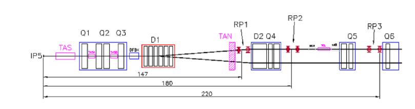
Figure 2: The TOTEM lay-out of leading proton detectors (Roman Pots). The detector locations at $\pm 147$ m (RP1) and at $\pm 220$ m (RP3) are shown [61]. The location of RP2 is not part of the present design.

In Fig. 3, the acceptance of elastic protons is shown as a function of $-t$ for three different run scenarios. An acceptance down to $\sim 5\cdot 10^{-3}\$ GeV² is achieved with the nominal LHC beam emittance; with improved beam emittance an acceptance down to $-t_{min}=2\cdot 10^{-3}\$GeV² is obtained [62]. Contrary to the nominal TOTEM optics, the $\beta^{*}=90\$m optics uses the standard LHC injection optics and could be realised during the run-in phase of the machine. The acceptance in $-t$ reaches $-t_{min}\approx 3.0\cdot 10^{-2}\$GeV².

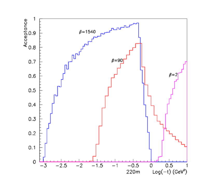
Figure 3: $-t$ acceptance of elastic protons detected at $\pm 220$ m from the IP5 for the ’nominal’ ($\beta^{*}=1540$ m) and for two ’custom’ run options ($\beta^{*}\simeq 90\$m.) [62].

Due to the geometric constraints imposed by the LHC vacuum pipe and beam screen, elastic protons with $-t$ values in excess of $0.5\$GeV² cannot be measured with the nominal high-$\beta^{*}$ optics conditions. Also, since at high $-t$ values $d\sigma_{el}/dt\propto 1/t^{8}$, higher luminosities would be desired. The “standard” LHC optics scenario includes the “injection” optics with $\beta^{*}=11\$m and a “pilot” stage optics with $\beta^{*}=2\$m that allows elastic protons with higher $-t$ values to be accessed (Figure 3). With the $2\$m optics, a reasonable event statistics up to $-t=10\$GeV² ($15\$GeV²) and resolution $\sigma(|t|)/|t|\approx 2\%$ is achieved.

With the high-$\beta^{*}$ TOTEM optics, so-called parallel-to-point focussing conditions are achieved (at $\pm 220\$m in both horizontal and vertical planes) and the elastic proton measurement becomes independent of the location of the primary interaction vertex. This will reduce systematic uncertainty in measuring the four-momentum-transfer squared of the scattered proton.

The angular beam divergence dominates the uncertainty in measuring -t, and together with the detector resolution, accounts for basically all of the uncertainty in $-t$. For small values of $-t$ ($-t=0.01\$GeV²) the error in $-t$, $\Delta t/t$, is $\sim 3\%$ in case the forward-backward pair of leading proton measurement stations is used and $\sim 5\%$ if only one of the two leading proton spectrometry “arms” is used.

With lower center-of-mass energies, the acceptance in $-t$ improves and, at the energies of $\sqrt{s}=2\$TeV, $-t$ values of one order of magnitude lower than at the nominal LHC energy are reached. This would allow comparisons with the Tevatron results and the Coulomb-hadronic interference region to be probed.

2.2 Extrapolation to the optical point

For the total pp cross section measurement, extrapolation of the elastic scattering $t$ distribution, $dN_{el}/dt$, to $t=0$ is required. The relative statistical uncertainty of the extrapolation is estimated to be $~{}0.1\%$ based on short periods of data taking with the nominal TOTEM optics and luminosity of $10^{28}\$cm^-2$s^{-1}$ [61].

A thorough study of the systematical effects in the extrapolation process was carried out [61, 62] and concluded that a precision better than $0.5\%$ should be achieved in extrapolating the elastic cross section to the optical point.

In case Coulomb scattering is not accounted for in the extrapolation process, a shift of $(d\sigma_{el}/dt)|_{t=0}\$of $(1\div 2)\%$ could occur. Due to Coulomb scattering contribution, the slope $B$ in $d\sigma_{el}/dt\sim\exp(Bt)$ does not stay constant at low $-t$ as assumed in a usual extrapolation. The uncertainty due to this effect might represent an uncertainty of several parts in $10^{-3}$ to the extrapolation.

2.3 Measuring $\rho$

For measuring the $\rho$-parameter,

$$\rho={\Re A(s,t=0)\over{\Im{A(s,t=0)}}},$$ (7)

one fits the elastic differential cross section:

$$\frac{1}{L}\frac{dN_{el}}{dt}=\frac{d\sigma}{dt}=\frac{4\pi\alpha^{2}F_{1}^{4}(t)}{t^{2}}-\frac{\alpha(\rho+\Delta\phi)\sigma_{tot}F_{1}^{2}(t)}{|t|}e^{-B|t|/2}+\frac{\sigma_{tot}^{2}(1+\rho^{2})}{166\pi}e^{-B|t|},$$ (8)

where the three terms are due to Coulomb scattering, Coulomb-hadronic interference, and hadronic interactions. $L$ is the integrated luminosity, $\alpha$ the fine structure constant, $\Delta\phi$ the relative Coulomb-hadronic phase, given as

$$\Delta\phi=-\ln(B(s)|t|/2)-0.577$$ (9)

and $F_{1}(t)$ is the nucleon electromagnetic form factor, which is usually parameterized as

$$F_{1}(t)=\frac{1}{(1+|t|/0.71)^{2}}.$$ (10)

In the least squares fit procedure, the following two equations are also used:

$$\sigma_{tot}^{2}=\frac{1}{L}\frac{16\pi}{(1+\rho^{2})}\frac{dN_{el}}{dt}|_{t=0};$$ (11)

$$\sigma_{tot}=\frac{1}{L}(N_{el}+N_{inel}).$$ (12)

Eq. (11) is a direct consequence of the Optical theorem. $N_{el}$ is the total number of events obtained by integrating the $dN_{el}/dt$ distribution within the $-t$ region where hadronic interactions dominate, and extrapolated to $-t=0$ and to $t\rightarrow\infty$ by using the form $\exp(-B|t|)$. $N_{inel}$ is the total number of inelastic events. Note that Eqs. (11) and (12) allow the luminosity $L$ to be expressed in terms of $\sigma_{tot}$ and $\rho$. Then $dN_{el}/dt$ in Eq. (8) can be expressed in terms of just three unknowns: $\sigma_{tot}$, $B$ and $\rho$. In the fit procedure, the same data on $dN_{el}/dt$, together with the total number of inelastic events $N_{inel}$ recorded during the same experimental data taking runs, are used as inputs. A least-squared analysis for $\sigma_{tot}$, $B$ and $\rho$ in Eq. (8) is done by using all the collected input data.

The evaluation of systematic errors due to the uncertainty in beam emittance, vertex positions and spread, beam transport and incoming beam angles is based on Monte Carlo and machine simulations. These simulations use the geometry of the experimental set-up and efficiency of the detectors as input.

2.4 Elastic scattering run scenarios

For elastic scattering, three run scenarios are considered (Table 1):

1. Nominal TOTEM optics for (low $-t$) elastic scattering, $\beta^{*}\sim 1500\$m,

2. An early medium- $\beta^{*}$ optics, with $\beta^{*}\cong 90\$m, and

3. Optics for large $-t$ elastic scattering, $\beta^{*}=2-0.55\$m.

The event rate per bunch crossing is calculated as (for symbols see Table 1)

$$N_{ev}=\frac{\sigma_{el}\ L}{f\ N_{b}}\left(\frac{N_{B}}{N_{b}}\right),$$ (13)

where $\sigma_{el}=$ elastic cross section, $L=$ luminosity, $f$ frequency, $N_{b}=$ no. of bunches; factor ($N_{B}/N_{b}\approx 1$) accounts for the empty buckets.

Scenario	1	2	3
	low $|t|$ elastic,	low $|t|$ elastic,	large $|t|$ elastic,
Physics:	$\sigma_{tot}$(@$\sim 1\%$),	$\sigma_{tot}$(@$\sim 5\%$),	hard diffraction
	MB, soft diffr.	MB, soft diffr.
$\beta^{*}$[m]	$\sim 1500$	$90$	$2\div 0.5$
N of bunches	$43\div 156$	156	$936\div 2808$
Bunch spacing [ns]	$2025\div 525$	$525$	$25$
N of part. per bunch	$(0.6\div 1.15)\cdot 10^{11}$	$1.15\cdot 10^{11}$	$1.15\cdot 10^{11}$
Half crossing angle [$\mu rad$]	$0$	$0$	$92$
Transv.norm.emitt. $\epsilon_{n}$[$\mu mrad$]	$1$	$3.75$	$3.75$
RMS beam size at IP [$\mu m$]	$450$	$213$	$32$
RMS beam diverg, at IP [$\mu rad$]	$0.3$	$2.3$	$16$
Peak Luminosity $[cm^{-2}s^{-1}]$	$10^{28}\div 2\cdot 10^{29}$	$3\cdot 10^{30}$	$10^{33}$

Table 1: Three different LHC run scenarios foreseen for elastic scattering measurements at the LHC.

2.5 Total $pp$ cross section measurement strategy

The total proton-proton cross section is measured - in a luminosity independent way - by using the Optical theorem. By extrapolating the elastic rate down to the Optical point, $t=0$, and by recording the elastic and inelastic event rates, the total cross section is measured with an over-all accuracy better than $1\%$.

For the total cross section measurement, the “nominal” TOTEM beam optics ($\beta^{*}\sim 1500\$ m) with several short runs is used. During the initial LHC running, the run scenarios with $\beta^{*}\simeq 90\$m is planned to be used for a total cross section measurement with an accuracy of about $5\%$.

For measuring the total cross section, inelastic scattering needs to be studied within large $E_{T}.$ The aim of the forward physics initiatives at the LHC is to complement the base line ATLAS (ALFA), CMS (TOTEM) and ALICE designs with forward detector systems (see Refs. [64, 65, 66, 67, 68] ). Besides restricted detector acceptance, inadequate theoretical understanding of the forward physics phenomena poses a serious systematic uncertainty for the base line experiments in need of precise luminosity measurement. As an example, the single diffractive cross section for the low diffractive mass region, $M^{*}<5\$GeV, could amount to $25\%$ of the over-all $\sigma_{sd}$ and cause a major systematic uncertainty in the total $pp$ cross section measurement.

The base line LHC experiments define a “minimum bias” event category that must be suppressed due to the limitations in recording $pp$ interactions in excess of the rate ($1^{st}$ level trigger band width) which can be recorded, as the cost of triggering on “interesting” large $E_{T}$ events. The main task of equipping the forward region of a main stream LHC experiment is to complement the physics reach by including the events that are not selected by the “minimum bias” event trigger. The TOTEM experiment together with CMS forward detectors (CASTOR, ZDC, and the proposed FSC and FP420 systems), represent the necessary complement for selecting an unbiased (!) sample of “minimum bias” events required for the analysis goals stated in the CMS Physics TDR.

In general, the soft particles in the non-diffractive event category (nd) will end up at central rapidities, while the relatively few energetic ones are expected to end up at small angles, to be recorded by the forward calorimetry and spectrometers.

The longitudinal, $z$, coordinate of the vertex is defined by first determining the distance of closest approach to the nominal $z$ axis for each track, $z_{track}$, (at least two tracks are required) and by then calculating the mean: $z_{vx}=<z_{track}>$ . By using this simple method, the $z$ coordinate of the primary interaction vertex can be determined with a resolution of $\sigma_{vx}\sim 5\$cm. The beam related events are identified by requesting that their reconstructed $z_{vx}$ value is within $\pm 50\$cm of the nominal IP. This selection is found to be more than $96\%$ efficient in choosing the beam related events. The remaining events have diffractively excited systems with relatively small masses, $M^{*}<10\$GeV, in which all the charged tracks escape detection in TOTEM T1 and T2 spectrometers (Figure 4).

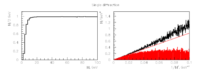
Figure 4: Left panel: Ratio of detected single diffractive (sd) events as a function of diffractive mass. Right panel: uncorrected Monte Carlo simulated (unshaded) and acceptance corrected (shaded) sd events with diffractive masses above 10 GeV [61].

For obtaining the over-all inelastic rate, the missing coverage above $\eta>7$ was estimated by extrapolation. Fig. 4 (right panel) shows the simulated $1/M^{*2}$ distributions for the single diffractive ($sd$) events before and after acceptance correction. A linear fit is used to correct for the unseen part of spectrum. In the case of $sd$ events, a correction of $4\%$, corresponding to about $0.6\$mb, was quoted above the detected fraction of this category of events. A similar analysis gives a correction factor of $0.1\$mb for double diffractive and $0.02\$mb for the central diffractive events [61].

Unfortunately diffractive cross sections are poorly known and theoretical understanding of both small and large mass single diffraction is lacking. Low mass single diffraction ($M^{*}<5\$ GeV) could represent $25\%$ of the total diffractive cross section (for double diffractive ($dd$) events the uncertainties are even more severe). Moreover, in the light of recent CDF measurements, soft central diffractive cross sections are likely to be seriously overestimated in current Monte Carlo models.

With the vertex constraint, a substantial part of the beam-gas events is rejected. The simulation studies [61] show that by using the vertex constraint, the beam-gas interactions closer than $\pm 5\$m represent only $\sim 3\%$ of the selected sample of events. Since the beam-gas event rate is estimated to be $2\$ Hz/m at $1/20$ of the nominal beam current, the trigger rate due to this source of background can be safely neglected. In addition, the Roman Pot based leading proton trigger $(\varepsilon\sim 90\%)$ can be used to further reduce the background rate.

2.6 $\sigma_{tot}$ measurement

The LHC (TOTEM) measurements of the total $pp$ cross section is luminosity independent and based on the Optical theorem:

$$\sigma_{tot}=\frac{16\ \pi}{(1+\rho^{2})}\frac{(dN/dt)_{t=0}}{N_{el}+N_{inel}},$$ (14)

where $N_{el}$ and $N_{inel}$ are the elastic and inelastic event rates, ($dN_{el}/dt$)$|_{t=0}$ is the elastic cross section extrapolated to the Optical point.

The relative error in $\sigma_{tot}$, neglecting uncertainty in $\rho$ , is then:

$$\left(\frac{d\sigma_{tot}}{\sigma_{tot}}\right)^{2}=\left(\frac{d(dN_{el}/dt)_{t=0}}{(dN_{el}/dt)_{t=0}}\right)^{2}+\left(\frac{d(N_{el}+N_{inel})}{(N_{el}+N_{inel})}\right)^{2},$$ (15)

The uncertainty in inelastic cross section is estimated to be less than 1 mb (see Ref. [61]). However, little experimental data on small mass diffraction exists, and the uncertainty in inelastic diffraction alone could amount to several millibarns. Together with the uncertainty of about $0.5\%$ of the extrapolated value of $(d\sigma_{el}/dt)|_{t=0}$, results in an over-all error of

$$\frac{\Delta\sigma_{tot}}{\sigma_{tot}}>>1\%.$$ (16)

The uncertainty in the value of the $\rho$-parameter could also have an important contribution to the $\sigma_{tot}$ measurement (see Chapter 3 and Ref. [69]), and it could be reduced by a direct measurement.

2.7 Luminosity measurement and monitoring

Luminosity measurement

The luminosity relates the cross section, $\sigma_{i}$, of a given process $i$ to the corresponding event rate $N_{i}$ by

$$L=\frac{N_{i}}{\sigma_{i}}.$$ (17)

It is not trivial to find a process with a well defined - and precisely calculable - cross section combined with a prominent event signature. The cross section should be large enough for monitoring the luminosity as a function of time, e.g. during a fill or when investigating bunch-to-bunch variations. By using several complementary aprroaches, systematic uncertainties can be brought under control [63].

A simultaneous measurement of the elastic and inelastic event rates can be used to define the luminosity as

$$L=\frac{1+\rho^{2}}{16\ \pi}\frac{(N_{el}+N_{inel})^{2}}{(dN_{el}/dt)|_{t=0})},$$ (18)

On-line luminosity monitoring

LHC is the first hadron collider where, due to the large c.m.s energy and high luminosity, a significant number of inelastic interactions (on average 35 interactions at the design luminosity) are expected to take place per bunch crossing. The traditional technique of monitoring luminosity by requesting a coincidence of two counters at small angles on both sides of the IP is not sufficient at the LHC. At the design luminosity, the coincidence rate observed will not be proportional to the number of events, but rather to the number of bunch crossings. In the case of no segmentation of the luminosity monitors, the probability to get a coincidence will be close to $100\%$.

Highly segmented forward detectors in T2 and/or FSC could be used as luminosity monitors. The rate used to monitor the luminosity, could be defined by using the double-arm coincidence rate between a pair of left-right detector segments. The segmentation reduces the counting rate significantly below the bunch crossing frequency and, therefore, becomes proportional to the luminosity. A coincidence signal between a pair of left-right detector segments is unlikely in case of separate overlapping $pp$ collisions. The technique would help to suppress beam related backgrounds. In principle, beam related background may be recognized by a time stamp given by a forward detector. During the beam cross-over at the IP, no other bunches should pass through the luminosity monitor location. Secondary particles from beam-gas and beam-wall interactions are traveling in-time with the bunch. In practice, the time stamping is challenging due to the high bunch crossing frequency (40 MHz). By requiring simultaneous left-right signals contributions from the beam related backgrounds are practically eliminated.

The calibration of the luminosity monitors can be performed during the dedicated high-$\beta^{*}$ runs at lower luminosities, where the luminosity is precisely determined together with tot. Alternatively, once the total inelastic cross section is precisely measured during the high- $\beta^{*}$ runs, together with the elastic and total cross sections, the inelastic events could be used to re-calibrate the monitor during the low-$\beta^{*}$ running. This becomes important when any significant changes to the detector lay-out are made, e.g. when the outer detectors are dismantled after the first year of running.

3 Forward physics at the LHC

Forward, or soft physics, roughly speaking, is the synonym of diffraction - elastic and inelastic, the role of the latter increasing with increasing scattering angle (or momentum transfer).

Forward physics will play an important role in early runs of the LHC for at least two reasons. One is that measurements of basic quantities, such as the total cross section $\sigma_{tot}(s)$, the ratio $\rho(s)$ of the real part to the imaginary one of the forward scattering amplitude, the local slope $B(s,t),$ of the differential cross section, etc. are of fundamental importance for the calibration/normalization of the beam and detectors and this task goes beyond the problems of understanding the nature of diffraction. Secondly, apart from classical studies of diffraction (Pomeron), the diffractive medium (gluons) may also favour central production of the Higgs boson. With increasing luminosity, the experiments at LHC will gradually shift towards measurements of rare events in the non-forward direction.

At the LHC, three collaborations, namely TOTEM/CMS, ALICE and ATLAS, are preparing to measure elastic, inelastic and the total $pp$ cross section at the expected energy $\sqrt{s}=14$ TeV. The complementarity of the expected performances will ensure optimal reliability of the results. The total cross section is claimed to be measured within $1\%$ of precision. The precision of the extrapolation to the optical point has been analyzed in [70]

One should note that the predictions based on model extrapolations for $\sigma_{tot}^{pp}$ at $\sqrt{s}=14$ TeV have a wide range. For example, Landshoff predicts [1, 2] $\sigma_{tot}^{pp}$ (14 TeV) $=(125\pm 25)$ mb.

TOTEM, CMS and FP420 collaborations are combining their efforts to cover a phase space (see Fig. 2), where the geometric acceptance of detectors is shown) exceeding that in any of the preceding collider experiment [67, 71, 72].

The TOTEM experiment, in particular, aims at measuring 1) the total proton-proton cross-section with a relative precision of about $1\%$; 2) the elastic proton-proton scattering between $10^{-3}$ GeV${}^{2}<-t\approx(p\Theta)^{2}<10$ GeV², $p$ and $\Theta$ being respectively the proton momentun and scattering angle in the c.m.s. Furthermore, by combining TOTEM with CMS and its forward additions, the CASTOR and ZDC calorimeters, a full forward physics program is planned.

The TOTEM experiment will measure $pp$ elastic scattering to about $-t=0.15\$GeV² and will provide crucial new understanding of the phenomena in the high $-t$ elastic scattering regime. To discriminate between different models, it is important to measure elastic scattering in the widest possible kinematic region. In most of the previous measurements of the total cross section (at ISR, SPS, Tevatron, RHIC) the value of the parameter $\rho$ was imported either from another experiment or from model calculations. As argued in Refs. [72, 73], known variations of the value of $\rho$ have a negligible effect on the resulting value of $\sigma_{tot}$. This is in disagreement with Ref. [74], where it was argued that a small variation of $\rho$ may affect the resulting $\sigma_{tot}$ significantly. If this is true, a simultaneous fit to all inputs ($\sigma_{tot},\rho,$ and ${\cal L}$) from a single experiment is needed. Publication of direct and unbiased data on ${sd-dN/{dt}}$ is highly welcome.

There are two possible kinds of luminosity measurements: one yields an absolute value which serves as a point of reference, the other one gives a relative value as a function of time. The latter measurement will be performed by ATLAS using a special detector called LUCID (Luminosity measurements Using Cherenkov Integrating Detectors). The idea of the LUCID detector is explained e.g. in Ref. [75]. It makes possible measurements in the very forward region, directly related to the instantaneous luminosity. This detector will enable ATLAS to obtain a linear relationship between luminosity and the number of tracks counted in the detector, directly related to the luminosity (see Table 2).

Measurements in the Coulomb-nuclear interference (CNI) region,

$$-t\sim 6.5\cdot 10^{-4}\ {\rm GeV}^{2},\ \ \Theta_{min}\sim 3.5\;\mu rad,$$

(note that at SPS $\Theta_{min}\sim 120\;\mu rad$) will be be used to extract the value of the parameter $\rho$ from Eq. (8).

The extracted value of $\rho$ may be affected by at least two phenomena. One is connected with the well known corrections [77] to the Coulomb-hadron phase [78] and the other one with the non-exponential behavior of the diffraction cone, known as the “fine structure of the Pomeron trajectory” [23, 24, 25, 39, 40, 41, 42]. Below, in Sec. 4, we shall come back to this point. The program of studying this “fine structure of the Pomeron trajectory” is among the priorities of the ATLAS collaboration [73, 75].

The ALICE experiment is designed as a general purpose experiment with a central barrel covering the pseudorapidity range $-0.9<\eta<0.9$ and a muon spectrometer covering the range $-4.0<\eta<-2.5$ at luminosities ${\cal L}=5\cdot 10^{30}cm^{-2}s^{-1}$ and ${\cal L}=10^{27}cm^{-2}s^{-1}$ in $pp$ and $PbPb$ collisions, respectively, as well as an asymmetric system $pPb$ at a luminosity ${\cal L}=10^{29}cm^{-2}s^{-1}$ (see, also, Ref. [79, 80, 81]).

Moreover, the experimental program of ALICE to large extent will be oriented to inelastic reactions, e.g. by studying their dependence on the width of the rapidity gap.

It should be noted that all these values are approximations since some of them were taken at $t=0$ as $\rho(0)$, $dN_{el}/dt\mid_{t=0}$, or integrated over all the region of angles as $N_{el}$, $N_{inel}$, i.e. all these values were obtained under some theoretical assumptions.

	input	fit	stat.error
${\cal{L}}$	8.10  1026	8.151  1026	1.77 %
$\sigma_{tot}$	101.5   mb	101.14   mb	0.9%
$B$	18 GeV-2	17.93   GeV-2	0.3%
$\rho$	0.15	0.143	4.3 %

Table 2: Result of a fit (see Ref. [76]) to simulated $dN/dt$ data corresponding to $\sim$ 1 week ($10\ M$ events) of running. ${\cal L}=10^{27}cm^{-2}s^{-1}$.

$\sqrt{s}$	$\sigma_{tot}$	$\delta\sigma_{tot}$	Authors	publication
540	66.800	5.90	ARNISON 83	PL 128B, 336
541	66.000	7.00	BATTISTON 82	PL 117B, 126
546	63.000	2.10	AUGIER 94	PL 344B, 451
547	61.260	0.93	ABE 93S	PR D50, 5550
900	61.90	1.50	BOZZO 84B	PL 147B, 392
1800	65.30	0.70	ALNER 86	ZP C32, 153
1800	71.42	1.55	AVILA 02	PL 537B, 41
1800	80.03	2.24	ABE 93S	PR D50, 5550
1800	72.80	3.10	AMOS 91B	PRL 68, 2433

Table 3: Range of the measured values of $\sigma_{tot}$ above the ISR energies

Tables 3 and 4 [82] show the range of the measured and the expected values of $\sigma_{tot}$ above the ISR energies, with the divergence of the existing data on $\sigma_{tot}$ at the same energy quoted in Table 2. One can see that the extraction of $\sigma_{tot}$ from the differential cross section $dN/dt$ is a complicated problem and that the use of different models can chance the predicted value of the total cross sections at the LHC energies from $80$ mb to $230$ mb (see Table 3). Therefore, one cannot use the theoretical predictions of, say $\sigma_{tot}$ or $\rho$, to extract other observables from the experimental data on $dN/dt$. With the exception of the UA4 and UA4/2 Collaborations, the numerical data on $dN/dt$ of other collaborations were not published, excluding any cross-check or improvement of these results. We hope that the future LHC data on $dN/dt$ will be published.

In Ref. [75] the significant correlations between the values of $\rho$ and $\sigma_{tot}$ are also visible. The results of the fits of the simulated LHC experimental data in the framework of the non-exponential model of the hadron scattering amplitude presented at “EDS-07” [82] at $\sqrt{s}$ equal to $2$ TeV and $14$ TeV show large errors in the determination of $\sigma_{tot}$ and $\rho(0)$ (see Tables 3 and 4).

Collaboration		$\sigma_{tot}$ (mb)	$\sigma_{el}/\sigma_{tot}$	$\rho(t=0)$	$B(t=0)$
KMR	[85]	88.0 (86.3)	0.22 (0.209)	-	-
C. Bourrely et al	[83]	103	0.28	0.12	19
E. Gotsman et al	[84]	110.5	0.229	-	20.5
COMPETE Coll.	[86]	111	-	0.11	-
B. Nicolescu et al	[87]	123.3	-	0.103	-
S. Goloskokov et al	[88, 89]	128	0.33	0.19	21
J.R. Cudell et al	[90]	150	0.29	0.24	21.4
Petrov et al	[91]	230	0.67	-	-
V. Petrov, A. Prokudin	[92]	107	0.28	0.138	-
M. Islam et al	[93]	110	-	0.12	-

Table 4: Predictions of the parameters of elastic scattering amplitude at $\ (\sqrt{s}=14\$TeV, $t=0$)

The (weak) dependence of $\sigma_{tot}$ on $\rho,$ if $\rho$ is very small, and it comes from the coefficient $1/(1+\rho^{2})$ in front of $d\sigma/dt$ (see Eq. (14)), while the strong dependence of the normalization of $dN/dt$, the values of $\sigma_{tot}$ and $\rho(0)$ comes from the extraction of the Coulombic and Coulomb-hadron interference terms from $dN/dt$ data to obtain $(d\sigma_{el}/dt)_{t=0}$. The Coulomb-hadron interference term is proportional to $[\rho(s,t)-\alpha\Phi_{cn}(s,t)]$. At very small $t,$ the Coulomb-hadron phase is also important. Corrections to the Bethe formula [94] were calculated in Refs. [95, 96, 97, 98]. A detailed analysis of the role of this term in the behaviour of the differential cross sections was carried out in Ref. [92]. To make the analysis complete, the Odderon contribution [23, 24, 25] as well as the nearby threshold singularity at $t=4m_{\pi}^{2}$ [39], should be also taken into account.

To minimize the errors, in some experiments the value of $\sigma_{tot}$ or $\rho$ were fixed from other measurements. This was done, for example, by the UA4/2 Callaboration, which extracted $\rho(0)$ by using $\sigma_{tot}$ from the result of the UA4 Collaboration ($\sigma_{tot}=61.9$ mb). However, the value of $\sigma_{tot}$ obtained by the Collaboration UA4/2 turned out to be $\sigma_{tot}=63.0$. With such a value of $\sigma_{tot}$ the resulting $\rho(0)$ becomes larger. This situation was analysed in Refs. [99, 69]. with the results shown in Table 5.

Diffraction dissociation, in particular the low mass one, is among priorities of the first experiments at the LHC. It should be remembered that diffraction dissociation - both single and double - and elastic scattering have much in common. Similarities are expected in the shape of the diffraction cone, with its fine structure (the “break” and oscillations), open for observation, see Ref. [100], and the dip-bump structure (until now not seen in diffraction dissociation). Hence studies of elastic scattering and diffraction dissociation are complementary. A recent overview of the ALICE detector and trigger strategy for diffractive and electromagnetic processes at the LHC can be found in Ref. [79, 80, 81].

${\rho}\ (\sqrt{s}=540\$GeV, $0.000875\leq|t|\leq 0.12\$GeV2)
n	experiment	exp. analysis	mod. anal. I [99]	mod. anal. II [69]
1	UA4	$0.24\pm 0.02$	$0.19\pm 0.03$	-
2	UA4/2	$0.135\pm 0.015$	-	$0.17\pm 0.02$

Table 5: Comparison of experimental values of the ratio $\rho$ of the real to imaginary part of the scattering amplitude, obtained in the UA4 and UA4/2 experiments, with theoretical values.

4 The forward cone

4.1 The “break” at very small $|t|$

An essential part of the future TOTEM+CMS and ATLAS experiments is connected with the measurement of the elastic differential cross section at small momentum transfer, with the purpose of extracting from these data the values of the total cross section. An important point of this procedure is the simultaneous measurement of four quantities: the luminosity $L$ (or the normalization coefficient), the total cross section $\sigma_{tot}$, the slope $B(s,t)$, defined as

$$B(s,t)={\frac{d}{dt}}\log{\frac{d\sigma(s,t)}{dt}}$$ (19)

and the ratio $\rho$. The last two quantities depend on their, a priori unknown, $t$-dependence. Consequences of this complexity are the contradictions of the obtained values of $\rho(s)$ in different experiments in the energy range of $\sqrt{s}=5\div 20\$GeV [99], in particular the large difference in the values of $\rho$ as measured in the UA4 and UA4/2 experiments at $\sqrt{s}=540\$GeV as well as the discrepancy between the values of $\sigma_{tot}$ at $\sqrt{s}=1.8\$TeV. This discrepancy results from the correlations between simultaneous measurements of several unknown values in a single experiment instead of fixing some values from the phenomenological analysis or from other experiments.

This situation was demonstrated for example in Ref. [99]. Since we do not know the true $t$-dependence of $\rho$ and of $B$, one cannot use the same constant values for different small intervals of $t$. Therefore, simultaneous measurements of all unknown observables in a single experiment are needed, rather than their substitution by values taken either from phenomenological models or alternative experiments, as illustrated e.g. in Refs. [99, 69], where compatible values of $\rho$, different from those experimental were obtained.

Given the uncertainty in the $s$ and $t$ dependence of the observables, the standard procedure is to suppose their smooth and monotonic behavior from low to super-high energies. Along these lines, it is usually proposed to measure $\sigma_{tot}$ taking the value of $\rho$ from the results of theoretical analysis (for example, that of the COMPETE Collaboration [86]), although, as argued in Refs. [3, 4, 5, 6], any consistent analysis should include a simultaneous fit to expression of Eq. (8).

In the ISR energy region, the $pp$ diffraction cone changes its slope $B(s,t)$ near $t=-0.1$ GeV² by about 2 units of GeV^-2. In Ref. [39] this phenomenon was interpreted as the manifestation of $t-$channel unitarity (a two-pion loop, see Fig. 1) and, in term of the Pomeron exchange, it was modeled by the inclusion of a relevant threshold singularity in the trajectory:

$$\alpha_{P}(t)=\alpha_{0}+\alpha_{1}t-\alpha_{2}\sqrt{4m_{\pi}^{2}-t},$$ (20)

where $\alpha_{2}/\alpha_{1}\approx 0.1.$ It will be interesting to see whether this effect will persist at the LHC and thus confirm the idea of Ref. [39].

As shown in Ref. [100], the “break”, or the fine structure of the Pomeron, in principle, can be seen directly, unbiased by electromagnetic interactions, in proton-neutron scattering.

4.2 Oscillations

An important phenomenon that should be scrutinized at the LHC is the possible appearance of small-period oscillations over the smooth exponential cone. Possible deviations from a simple exponential behaviour of the hadron-hadron scattering amplitude were discussed in the literature long ago. For example, it was shown in Ref. [101] that peripheral contributions from inelastic diffraction result in large- and small-period oscillations in the momentum transfer. Among the attempts to verify these oscillations the first one was done in an experiment at Serpukhov, where oscillations in $pp$ scattering were detected [102] and then discussed in Ref. [103]. An alternative view, interpreting these oscillations as an artifact, connected with the $t-$ dependence of the slope, was put forward in Ref. [104]. In Ref. [105] the statistical nature of the possible oscillations in the ISR data were analyzed in the framework of the Dubna Dynamical (DD) model (for the DD model see Subsection 5.4). The results are shown in Fig. 5.

The effect was first observed at the ISR and subsequently was discussed in Ref. [106, 107]. Although it has not yet been confirmed unambiguously, it continues to attract attention (see Ref. [106, 107] and references therein). The analysis of the slope [106, 107] shows possible oscillations in the UA4/2 data. The super-fine structure (oscillations) of the cone may be related to residual, long-range interaction between nucleons [108] or the action of a potential of rigid hadronic strings [109].

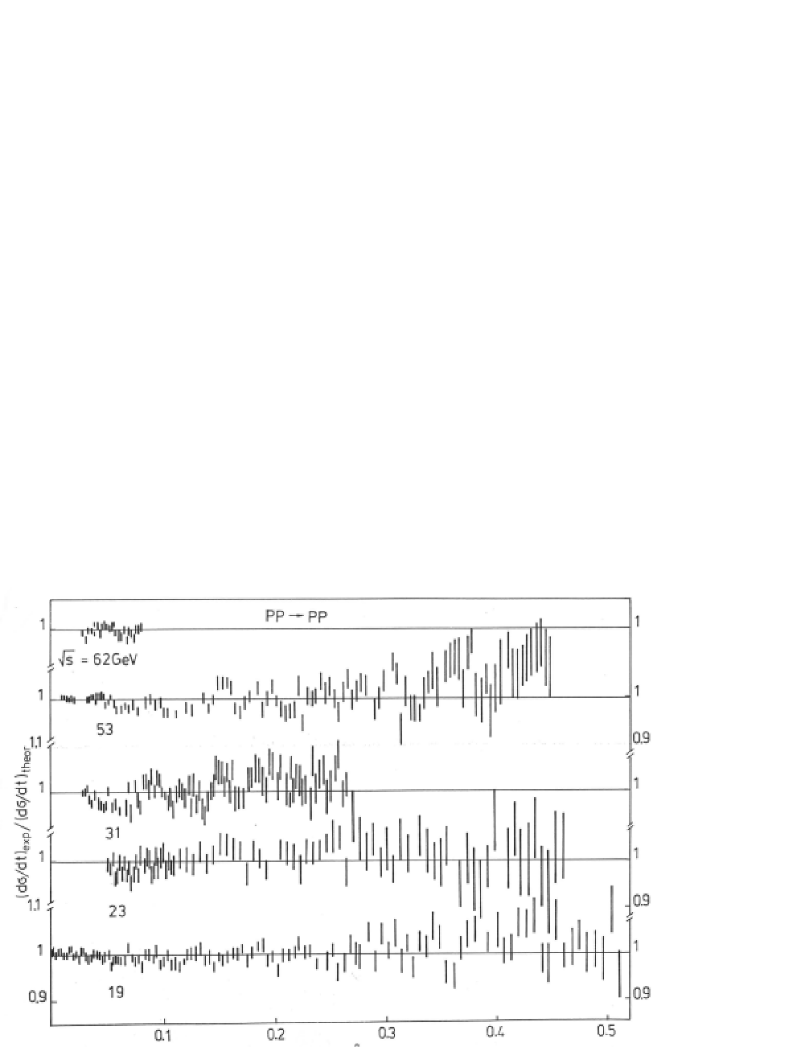
Figure 5: Ratio of the experimental differential cross section to theoretic one calculated from the DD model [105] in the ISR energy region.

A new method of the analysis of the experimental data of UA4/2 experiment was proposed in Ref. [110]. The method is based on the comparison of two statistically independent sets, Ref. [111]. If we have two statistically independent sets $x^{{}^{\prime}}_{n_{1}}$ and $x^{"}_{n_{2}}$ of values of the quantity $X$ distributed around a certain value, say $A,$ with the standard error equal to $1$, we can try to find the difference between $x^{{}^{\prime}}_{n_{1}}$ and $x^{"}_{n_{2}}$. For that we can compare the arithmetic mean of these choices:

$$\Delta X=(x^{{}^{\prime}}_{1}+x^{{}^{\prime}}_{2}+...x^{{}^{\prime}}_{n1})/n_{1}-(x^{"}_{1}+x^{"}_{2}+...x^{"}_{n2})/n_{2}=\overline{x^{{}^{\prime}}_{n_{1}}}-\overline{x^{"}_{n_{2}}}.$$

The standard deviation for this case will be

$$\delta_{\overline{x}}=[1/n_{1}+1/n_{2}]^{1/2}.$$

If we have the purely statistical noise the value $\Delta X/\delta_{\overline{x}}$ tends to zero. However if there is some additional signal, this value should differ from zero. When it is larger than $3$, one can say that the difference between these two choices has a $99\%$ probability of confirming the presence of the oscillations (for more details see Ref. [110]).

The deviation $\Delta R_{i}$ of each of the experimental data for the cross section from the corresponding theoretical values is measured in units of the experimental error $\delta_{i}^{exp}$:

$$\Delta R_{i}=[(d\sigma/dt_{i})^{exp}-(d\sigma/dt_{i})^{th}]/\delta_{i}^{exp}.$$ (21)

By summing these $\Delta R_{i}$ over all 99 experimental points of the UA4/2 experiment, the result should tend to zero as the statistical deviations are equally probable in both sides of the theoretical curve. However, if the theoretical curve does not precisely describe the experimental data, for example, the scattering amplitude deviates from the exponential behavior in the momenta transfer, the sum over $\Delta R_{i}$ can differ slightly from zero, going beyond the value of a statistical error. To take into account this effect, we divide the whole interval of the momentum transfer into $k$ equal pieces of size $\Delta$ such that $k\Delta\geq(q_{99}-q_{1})$, where $q_{i}=\sqrt{|t_{i}|}$, and sum $\Delta R_{i}$ separately over the even and odd pieces. Thus, we get two sums $L^{up}$ and $L^{dn}$ for the $n_{1}$ even and $n_{2}$ odd interval, respectively. For $n_{1}+n_{2}=k$ and $|n_{1}-n_{2}|=0$ or $1$:

$$L^{up}=\sum_{j=1}^{n_{1}}(\sum^{99}_{i}\Delta R_{i})|_{\Delta q(2j-1)<q_{i}\leq\Delta q(2j)};\ \ \ L^{dn}=\sum_{j=1}^{n_{2}}(\sum^{99}_{i=1}\Delta R_{i})|_{\Delta q(2j)<q_{i}\leq\Delta q(2j+1)}.$$ (22)

In Ref. [110], where this method was applied to the data of the UA4/c Collaboration, $\Delta q=0.9085\cdot 10^{-2}$ GeV was used.

Let us calculate the quantities $L^{up}$ and $L^{dn}$; the results are shown in Fig. 6 by the full and dash-dotted lines. It can be seen that in the range $0<|t|\leq 0.1$ GeV² these quantities change drastically and in the range $|t|>0.1$ GeV² instead they vary slightly. It means that the amplitude of a possible periodic structure is decreasing with growing $t$.

Figure 6: Left panel: Sums $L^{up}$ and $L^{dn}$ calculated [69] with $\sigma_{tot}=62.2\ mb;\ B=15.5\ GeV^{-2};\ \rho=0.135$ for $q_{0}$ and $\delta q$ (full and dashed lines); and for $q_{0}+\delta q/2$ ( dots and dots-dashed lines). Right panel: Same as on the left panel but with $\sigma_{tot}=63.54\ mb;\ B=15.485\ GeV^{-2};\ \rho=0.158$.

Note that this new method can be used to check the true determination of the parameters of the elastic scattering at small $t$. The two curves obtained have to be symmetric with respect to the line calculated by using the basic parameters ($\sigma_{tot},\rho,B$).

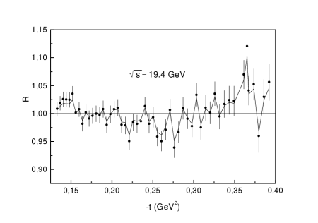
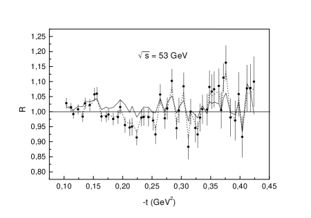
Figure 7: Left panel: $t-$ oscillations calculated in Ref. [106] as the ratio of the experimental to the theoretical values at $\sqrt{s}=19.4$ GeV. Data are from Ref. [112]. Right panel: Same as on the left panel but for the data from Ref. [113].

A way to identify possible oscillations at the LHC is to use the method of overlapping bins, suggested by J. Kontros and Lengyel in Ref. [106]. The procedure consists in scanning the cone by overlapping bins in $t$, each containing a certain number $N$ of data points shifted by a small number of points $n$. Within each bin an exponential fit is applied [106, 107] (see Fig. 7).

The length of the bin should not be too large to oversimplify the parameterization and not too small in order to contain a reasonable number of points for each process. For example, a shift from bin to bin $\delta t=0.01$ GeV² was found in Ref. [106] reasonable.

Looking for oscillations in the cone at LHC by using the method of overlapping bins of Ref. [106, 107] is a promising program for future experiments. As already mentioned, the oscillations can be related to residual long-range forces between nucleons [108].

5 The Dip-Bump Region, $t\sim-1$ GeV²

Before going into details, we would like to notice a model-independent regularity found in Ref. [114]. As shown in that paper, a correlation between the value of $\rho$ and the depths of the minima of the diffraction differential cross section in proton-proton and proton-antiproton scattering exists. The ratio $\rho$ for the latter changes sign in the energy region $\sqrt{s}=9.8\$GeV. At this energy the differential cross section of $p\bar{p}$-scattering in the dip-bump structure has its sharpest minimum, while $\rho$ in $pp$-scattering changes its sign around $\sqrt{s}\sim 30\$GeV. At this energy the differential cross section of $pp$-scattering has its sharpest minimum.

At the highest ISR energies all models and experiments show that $\rho(0)_{\bar{p}p}>\rho(0)_{pp}$. The experiments also show that the dip at these energies in $\bar{p}p$ is higher then in $pp$-scattering.

The observed dip-bump structure in the high-energy differential cross section was not predicted by any model or theory. It can be related e.g. to the multiple scattering of quarks and gluons (Glauber theory), leaving however much room for speculations on the basic inputs in this approach. The optical model (see Ref. [115] and earlier references therein) predicted a sequence of minima and maxima, however the ISR and SPS data show only one structure, both in $pp$ and in $p\bar{p}$ scattering. Some models [116] predict that more structure will appear at higher energies, for example at the LHC. The (non)appearance of additional minima and maxima at the LHC will confirm or rule out part of the existing models, although most of them will survive by refitting its parameters a posteriori.

Two models [22, 117, 118], fitted to the data in a wide range of $s$ and $t,$ can illustrate the state of art in this field (see, for instance, Fig. 8). While the authors of Ref. [22] claim that fits require the presence of an Odderon contribution, those of Ref. [117, 118] do not need it. By this we only want to stress that the flexibility of the existing models allow for good “postdictions”, but their predictions are not unique. In this situation useful empirical parameterization [119], unbiased by any theoretical prejudice can be useful.

Figure 8: Left panel: Elastic $pp$ differential cross section predicted in Ref. [117, 118]. Right panel: Elastic $pp$ and $p\bar{p}$ differential cross section predicted in Ref. [22].

By definition, any diffractive pattern in ${d\sigma}$/$dt$ is a property of the (predominantly imaginary) Pomeron contribution, rather than of the “non-diffractive” Odderon, whose amplitude is predominantly real and thus it can only “contaminate” the diffractive pattern.

5.1 A simple model of the diffraction pattern

Data on $pp$ scattering below the LHC energy region can be described by a Pomeron and sub-leading contributions. From the phenomenological point of view, the need for the Odderon, becomes important only after the SPS data on $p\bar{p}$ scattering appeared, in which the dip seen in $pp$ scattering appeared as a “shoulder”, suggesting that the diffractive minimum was filled by the Odderon contribution. This is not a proof, just a plausibility argument. Below we illustrate the dynamics of the dip and shoulder in $pp$ and $p\bar{p}$ scattering by using a simple (“minimal”) dipole Pomeron (DP) model to “guide the eye”. It reproduces the observed dynamics of the dip and will help to anticipate the LHC phenomena.

By neglecting spin effects, the scattering amplitude for $pp$ and $p\bar{p}$ scattering is written as a sum

$$A^{p\bar{p}}_{pp}(s,t)=P(s,t)\pm O(s,t),$$ (23)

where $P$ is the Pomeron contribution and $O$ is that of the Odderon. For the DP amplitude we use the following “minimal” model [23, 24, 120, 26, 27]

$$P(s,t)=i{as\over{bs_{0}}}\Bigl{(}r^{2}_{1}(s)e^{r^{2}_{1}(s)[\alpha_{P}(t)-1]}-\epsilon r^{2}_{2}(s)e^{r^{2}_{2}(s)[\alpha_{P}(t)-1]}\Bigr{)},$$ (24)

where $r_{1}^{2}(s)=b+L-{i\pi\over 2},\ \ r_{2}^{2}(s)=L-{i\pi\over 2}$ with $L\equiv\ln{s\over{s_{0}}}$; $\alpha_{P}(t)$ is the Pomeron trajectory and $a,b,s_{0}$ and $\epsilon$ are free parameters. The model produces rising cross sections without violation of the Froissart bound as well as a dip-bump structure seen in the $pp$ scattering with its non-trivial dynamics observed at the CERN ISR in the range $23<\sqrt{s}<62GeV$ [23, 24, 120, 26, 27]. The absence of a relevant structure (replaced by a “shoulder”) in $p\bar{p}$ scattering at the CERN SPS was interpreted [23, 24, 26, 27] as a manifestation of the Odderon, filling the dip produced by the Pomeron term (for reviews see Refs. [10, 38]). A high-quality description of elastic high-energy data with predictions for future accelerators can be found in [116]. In an alternative successful approach [121] there are several Pomerons, whose interference produces the dip-bump structure and perfect agreement with the data.

Since little is known about the properties of the Odderon, apart from its assumed asymptotic nature, one usually parameterizes it in the form close to that of the Pomeron given in Eq. (24). However: 1) the Odderon is $C-$ odd, which implies an extra $i$ factor in front of the amplitude; 2) its relative contribution is by orders of magnitude smaller than that of the Pomeron (until now the Odderon was not seen in the forward direction); 3) the slope of the Odderon trajectory is much smaller than that of the Pomeron. There are two reasons for the latter: one is based on theoretical arguments [23, 24] and the other one is phenomenological: the “flat” shoulder in $p\bar{p}$ scattering, seen at the SPS, could be a manifestation of the Odderon.

Let us remind that the dip in the ISR energy region is monotonically deepening, reaching its maximal depth at $52.8$ GeV, whereafter the monotonic trend changes, albeit at a single energy equal to $62$ GeV. Similar to the unique case of the measured [34, 35] difference between $pp$ and $p\bar{p}$ amplitudes at $53$ GeV, mentioned in the Introduction, this phenomenon needs confirmation. Regrettably, measurements of the difference between $pp$ and $p\bar{p}$ amplitudes are not foreseen in the near future.

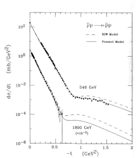
Figure 9: Differential cross section at $546$ and $1800$ GeV calculated from Eqs. (23) and (24) with the $P+O$ contribution, corresponding to $p\bar{p}$ scattering (full line), compared with those of Ref. [83] (broken line). For detail of the calculations see Refs. [23, 24, 26, 27, 120].

Fig. 9 shows the differential cross section of $p\bar{b}$ scattering at $546$ and $1800$ GeV calculated from Eqs. (23) and (24) (full line), compared with a fit from paper [83] (broken line). Details of the calculations and the values of the fitted parameters can be found in Refs. [23, 24, 26, 27, 120].

It should be reminded that the hypothetical Odderon contributes enters Eq. (6) with different signs in $pp$ and $p\bar{p}$ amplitudes, thus distorting the pure Pomeron contribution in both cases. Due to its small slope (flatness of its trajectory), the role of the Odderon increases with increasing $-t,$ the phenomenon reaching its maximum in the dip region.

The ratio of the cross section at the minimum to that at the maximum (depth of the dip) is more informative than its absolute value. Even greater than at the ISR ($\sim 5$) value of the ratio will indicate the monotonic deepening of the dip and will disfavour the Odderon contribution, while its shallowing will favour the presence of the Odderon.

At this point it may be appropriate to introduce several known models describing the diffractive pattern (the dynamics of the dip-bump structure). Before doing so, two points are worth mentioning: 1) one still lacks a theoretical understanding of the phenomenon and must rely on models; 2) among the large number of models, only few are able to fit properly the large number of high-statistics data that exist in a wide range of $s$ and $t$ for $pp$ and $\bar{p}p$ scattering. A collection/review of the existing models for high-energy scattering with a critical evaluation of their prediction is highly desirable, however this task is beyond the scope of the present paper. We apologize to those authors whose papers, for brevity of space, are not cited here.

5.2 The “Protvino” model

One of the examples of eikonal models of diffraction is the “Protvino” model [92, 121].

The unitarity condition

$$\Im{\rm m}\;T(s,\vec{b})=|T(s,\vec{b})|^{2}+\eta(s,\vec{b})\;,$$

where $T(s,\vec{b})$ is the scattering amplitude in the impact representation, $\vec{b}$ is the impact parameter, $\eta(s,\vec{b})$ is the contribution of inelastic channels, implies the following eikonal form for the scattering amplitude $T(s,\vec{b})$:

$$T(s,\vec{b})=\frac{e^{2i\delta(s,\vec{b})}-1}{2i}\;,$$ (25)

where $\delta(s,\vec{b})$ is the eikonal function. The unitarity condition in terms of the eikonal looks as follows:

$${\rm\Im m}\;\delta(s,\vec{b})\geq 0,\;s>s_{\rm inel}\;.$$ (26)

The eikonal function is assumed to have simple poles in the complex $J$-plane and the corresponding Regge trajectories are normally used in the linear approximation

$$\alpha(t)=\alpha(0)+\alpha^{\prime}(0)t\;.$$ (27)

The following representation for the eikonal function is used:

$$\delta_{pp}^{\bar{p}p}(s,b)=\delta^{+}_{{P}_{1}}(s,b)+\delta^{+}_{{P}_{2}}(s,b)+\delta^{+}_{{P}_{3}}(s,b)\mp\delta^{-}_{O}(s,b)+\delta^{+}_{f}(s,b)\mp\delta^{-}_{\omega}(s,b),$$ (28)

where $\delta^{+}_{{P}_{1,2,3}}(s,b)$ are Pomeron contributions. ‘$+$’ denotes C even trajectories (the Pomeron trajectories have the following quantum numbers $0^{+}J^{++}$), ‘$-$’ denotes C odd trajectories, $\delta^{-}_{O}(s,b)$ is the Odderon contribution (the Odderon is the C odd partner of the Pomeron with quantum numbers $0^{-}J^{--}$); $\delta^{+}_{f}$, $\delta^{-}_{\omega}(s,b)$ are the contributions of secondary Reggeons, $f$ ($C=+1$) and $\omega$ ($C=-1$).

The parameters of secondary Reggeon trajectories are fixed according to the parameters obtained from a fit of the meson spectrum:

$$\begin{array}[]{l}\alpha_{f}(t)=0.69+0.84t\;,\\ \\ \alpha_{\omega}(t)=0.47+0.93t\;.\end{array}$$ (29)

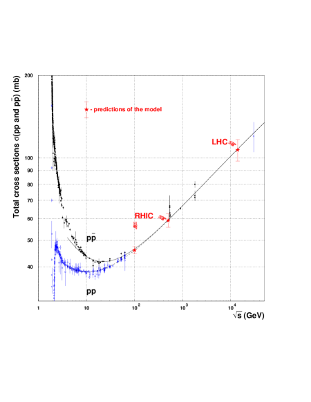
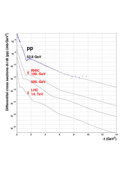
Figure 10: Left panel: Total cross sections of $pp$ scattering (hollow circles) and $\bar{p}p$ scattering (full circles) and curves corresponding to their description in the three-Pomeron model [121, 92]. Right panel: Predictions of the three-Pomeron model [121, 92] for the differential cross-section of $pp$ scattering to be measured at LHC with $\sqrt{s}=14.\;TeV$ and at RHIC $\sqrt{s}=100.\;GeV$ and $\sqrt{s}=500.\;GeV$. The data corresponding to the energy $\sqrt{s}=52.8\;GeV$ is multiplied by $10^{-6}$, RHIC at $500\$GeV by $10^{-10}$, RHIC at $500\$GeV by $10^{-12}$, and that of LHC by $10^{-16}$.

The model fits high-energy elastic $pp$ and $\bar{p}p$ scattering data. The data are well described for all momenta ($0.01\leq|t|\leq 14.\;GeV^{2}$) and energies ($8.\leq\sqrt{s}\leq 1800\$GeV) ($\chi^{2}/{\rm d.o.f.}=2.60$). It predicts the appearance of two dips in the differential cross-section which will be measured at LHC. The parameters of the Pomeron and Odderon trajectories are:
$\alpha(0)_{{P}_{1}}=1.058,\;\;\alpha^{\prime}(0)_{{P}_{1}}=0.560\;GeV^{-2};$
$\alpha(0)_{{P}_{2}}=1.167,\;\;\alpha^{\prime}(0)_{{P}_{2}}=0.273\;GeV^{-2};$
$\alpha(0)_{{P}_{3}}=1.203,\;\;\alpha^{\prime}(0)_{{P}_{3}}=0.094\;GeV^{-2}.$
$\alpha(0)_{{O}}=1.192,\;\;\alpha^{\prime}(0)_{{O}}=0.048\;GeV^{-2}.$

The model predicts (see Fig. 10) the following values of total and elastic cross sections at the LHC:

$$\sqrt{s}=14.\;TeV\;,$$

$$\sigma_{tot}^{pp}=106.73\;\;(mb)\;_{-\;8.50mb}^{+7.56\;mb}\;,$$ (30)

$$\sigma_{elastic}^{pp}=29.19\;\;(mb)\;_{-2.83\;mb}^{+3.58\;mb}\;,$$

$$\rho^{pp}=0.1378\;_{-0.0061}^{+0.0042}\;.$$

On the right panel of Fig. 10 one can see a typical “diffractive” pattern of the differential cross-section also present in other models based on unitarisation [122, 123, 124, 117, 118, 125] (see also Fig. 9 and Fig. 11).

5.3 The “Connecticut” model

A model based on a physical picture of the nucleon having an external cloud, an inner shell of baryonic charge, and a central quark-bag containing the valence quarks was proposed in Ref. [93]. The underlying field theory model is the gauged Gell–Mann – Levy linear $\sigma$-model with spontaneous breakdown of chiral symmetry, with a Wess–Zumino–Witten (WZW) anomalous action. The model attributes the external nucleon cloud to a quark–antiquark condensed ground state analogous to the BCS ground state in superconductivity – an idea that was first proposed by Nambu and Jona-Lasinio. The WZW action implies that the baryonic charge is geometrical or topological in nature, which is the basis of the Skyrmion model. The action further shows that the vector meson $\mathrm{\omega}$ couples to this topological charge like a gauge boson, i.e. like an elementary vector meson. As a consequence, one nucleon probes the baryonic charge of the other one via $\mathrm{\omega}$-exchange. In pp elastic scattering, in the small momentum transfer region, the outer cloud of one nucleon interacts with that of the other giving rise to diffraction scattering. As the momentum transfer increases, one nucleon probes the other one at intermediate distances and the $\mathrm{\omega}$-exchange becomes dominant. At momentun transfers even larger, one nucleon scatters off the other via valence quark-quark scattering.

Diffraction is described by using the impact parameter representation and a phenomenological profile function:

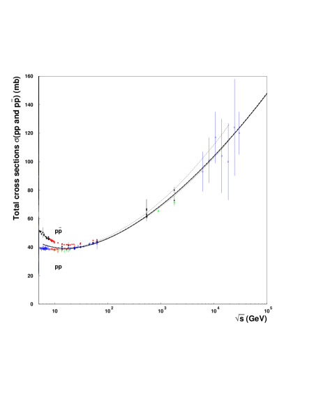
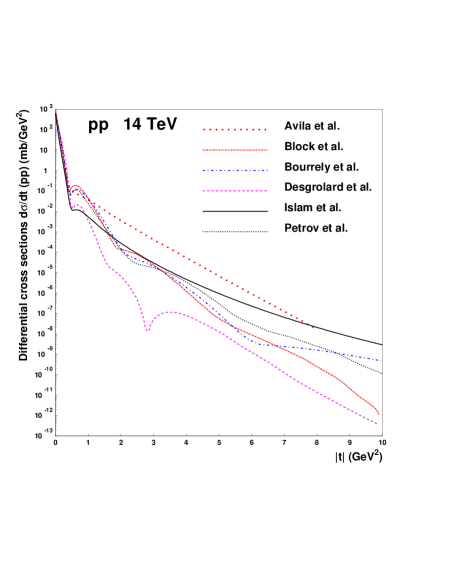
Figure 11: Left panel: Total cross sections of $pp$ scattering (open circles) and $\bar{p}p$ scattering (full circles) and the fitted curves based on the model [93]. Right panel: Predictions of the model [93] for the differential cross-section of $pp$ scattering to be measured at the LHC at $\sqrt{s}=14.\;TeV$ (solid line) and comparison with the prediction of other models: Avila et al. [22], Block et al. [126], Bourrely et al. [117, 118], Desgrolard et al. [127], and Petrov et al. (three pomerons) [92].

$$T_{D}(s,t)=i\,p\,W\int_{0}^{\infty}{b\;\rm{d}\it{b}\;J_{0}}(b\,q)\Gamma_{D}(s,b)\;.$$ (31)

here $q$ is the momentum transfer ($q=\sqrt{|t|}$) and $\Gamma_{D}(s,b)$ is the diffraction profile function, which is related to the eikonal function $\chi_{D}(s,b)$: $\Gamma_{D}(s,b)=1-\exp(i\chi_{D}(s,b))$. $\Gamma_{D}(s,b)$ is taken to be an even Fermi profile function:

$$\Gamma_{D}(s,b)=g(s)\left[\frac{1}{1+e^{(b-R)/a}}+\frac{1}{1+e^{-(b+R)/a}}-1\right]\;.$$ (32)

The parameters $R$ and $a$ are energy dependent:

$$R=R_{0}+R_{1}\left(\ln\frac{s}{s_{0}}-i\frac{\pi}{2}\right),$$

$$a=a_{0}+a_{1}\left(\ln\frac{s}{s_{0}}-i\frac{\pi}{2}\right);$$

$g(s)$ is a complex crossing even energy-dependent coupling strength, $s_{0}=1$ GeV².

For the diffraction amplitude the following asymptotic properties are obtained:

1. $\sigma_{\rm{tot}}(s)\sim(a_{0}+a_{1}\ln s)^{2}\hskip 80.23697pt$ (Froissart-Martin bound)
   

2. $\rho(s)\simeq\frac{\pi a_{1}}{a_{0}+a_{1}\ln s}\hskip 117.51001pt$ (derivative dispersion relation)
   

3. $T_{D}(s,t)\sim i\;s\;\ln^{2}s\;f(|t|\;\ln^{2}s)\hskip 48.93877pt$ (Auberson-Kinoshita-Martin scaling)
   

4. $T_{D}^{\mathrm{\bar{p}p}}(s,t)=T_{D}^{\mathrm{pp}}(s,t)\hskip 96.45482pt$ (crossing even)

At 14 TeV $\sigma_{tot}$ and $\rho_{pp}$ were found to have the values 110 mb and 0.120 mb, respectively.

Finally, Fig. 11 shows a compilation of predictions of the model for pp elastic $\rm{d}\sigma/d\it{t}$ at LHC together with the predictions of other models, e.g.: Avila et al. [22], Block et al. [126], Bourrely et al. [117, 118], Desgrolard et al. [127], and Petrov et al. (three pomeron) [92]. As one can see from Fig. 11, the model [93] predicts no diffractive pattern at large $|t|$ as diffractive scattering dominates in the small $|t|$ region, hard scattering dominates in the intermediate $|t|$ region ($1.5<|t|<8.0\;{\rm GeV^{2}}$) and quark-quark scattering takes over at large $|t|$.

5.4 The “Dubna Dynamical” model

The so-called “Dubna Dynamical” (DD) model was already cited in connection with the nearly forward scattering; it will be used also in Sec. 6.2 on the BDL, so we find it appropriate to briefly introduce it, especially as it may be closely related to models proposed earlier (see Refs. [117, 118, 122, 123, 124]) or later (see Refs. [93, 121, 92] and earlier references therein).

The DD model was developed in Refs. [125, 128, 129] to describe particle interaction with account for the internal structure of hadrons. According to the DD model, the hadron scattering amplitude can be written as a sum of a central and a peripheral part of the interaction [125]. The full scattering amplitude is calculated using the impact parameter representation with the eikonal form of the unitarization:

$$A(s,t)=is\int_{0}^{\infty}\ bdbJ_{0}(b\Delta)[1-e^{-\chi(s,b)}],$$ (33)

where

$$\chi(s,b)=\chi_{c}(s,b)+\chi_{p}(s,b)+\chi_{R}(s,b).$$ (34)

Here the central interaction term $\chi_{c}(s,b)$ describes the interaction between central parts of the hadrons. At high energies, it is determined by a spinless Pomeron exchange. The second term, $\chi_{p}(s,b)$ is the sum of triangle diagrams corresponding to the interaction of the central part of a hadron with the meson cloud of the other one. The meson-nucleon interaction leads to spin flip effects in the Pomeron-hadron vertex [114]. The term $\chi_{R}(s,b)$ describe the cross even and cross odd parts of the subleading Reggeons with the energy dependence $\sim 1/\sqrt{s}$.

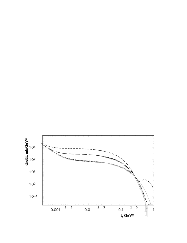
Figure 12: Predictions of the DD model [88, 89] for the Tevatron energies, $\sqrt{s}=1.8$ TeV (long dashed line) and for the LHC energies (short dashed line). For the sake of comparison, model curves and experimental data are shown for one lower energy, $\sqrt{s}=23$ GeV (solid line). The experimental data points are from Ref. [130].

The term $\chi_{c}(s,b$ ) was chosen phenomenologically (for details see Refs. [122, 123, 124]), where the scattering amplitude was obtained from an integral representation of the Bessel function. It was shown in those papers that, starting from the usual partial wave expansion in the Legendre polynomials, the eikonal representation for the scattering amplitude can be derived to be valid for all energies and in the whole angular domain, and for which the spectral function is given in terms of the partial wave amplitudes. The scattering amplitude can be presented in the form

$$A(p,\Theta)\approx-iB\alpha^{-\nu}\beta^{1-\nu}p{K_{\nu-1}[\beta(\alpha^{2}+p^{2}\sin^{2}\theta)^{1/2}]\over{\alpha^{2}+p^{2}\sin^{2}\Theta^{1-\nu}/2}}.$$ (35)

Although the analytic calculations can be performed to any $\nu$, to simplify numerical calculations, we set $\nu=1/2$, whereafter the amplitude becomes:

$$A(p,\Theta)=-i(\pi/2)^{1/2}\alpha^{-1/2}Bp{\exp[-\beta(\alpha^{2}+p^{2}\sin^{2}\theta)^{1/2}]\over{\alpha^{2}+p^{2}\sin^{2}\Theta^{1-\nu}/2}}.$$ (36)

By taking this form as the Born amplitude, the eikonal term $\chi_{0}$ in the DD model assumes the form

$$\chi_{0}(s,b)=A_{0}\ e^{-m(s)\ \sqrt{R_{0}^{2}+b^{2}}}.$$ (37)

It leads to an exponential behavior of the eikonal at large values of the impact parameter and a Gaussian behavior at small impact parameters. In the DD model the inelastic states in the $s$-channel were also taken into account. Accordingly, the central part can be presented as

$$\chi_{c}(s,b)=\chi_{0}(s,b)\ [1-\gamma\chi_{0}(s,b)],$$ (38)

with

$$\chi_{0}(s,b)=A_{0}\ e^{-m(s)\ \sqrt{R_{0}^{2}+b^{2}}}.$$ (39)

The coefficient $\gamma$ is connected with the contribution of the inelastic intermediate state in the $s$-channel. Here $A_{0},\ m(s)$ and $\ R_{0}$ are free parameters, whose values and energy dependence were determined from fits to the experimental data on proton-proton elastic differential cross section scattering from $\sqrt{s}=9.78\$GeV to $\sqrt{s}=540\$GeV (see Fig. 12) and momentum transfer from $t=0$ to $t=-12\$GeV².

The additional term $\chi_{p}$ was determined by the peripheral Pomeron interaction with account for the meson cloud. This leads to the important feature of the DD model, namely the existence in the eikonal phase of a small term growing as $\sqrt{s}:$

$$\chi_{p}(s,b)=H_{p0}+\lambda\sqrt{s}\ m_{p}\sqrt{R_{p}^{2}+b^{2}}K_{1}(\ m_{p}\sqrt{R_{p}^{2}+b^{2}}),$$ (40)

where $K_{1}$ is the MacDonald function of the first order. So, the contribution to the eikonal phase growing as $\sqrt{s}$ is determined by the peripheral meson-cloud effects. It has been shown that this term becomes important for energies $\sqrt{s}>200\$ GeV. The corresponding form of the interaction potential can be represented, see Ref. [122], by a superposition of Yukawa-like potentials in the form of the MacDonald function. The leading term of the $\chi_{c}$ in the momentum transfer representation is

$$\sim{\ e^{-R_{0}\ \sqrt{4m_{p}^{2}+q^{2}}}\over{\sqrt{4m_{p}^{2}+q^{2}}}}.$$ (41)

It results in the following form of the differential cross section for $q^{2}>>m_{p}^{2}$ [125]

$$\frac{d\sigma}{dt}\sim\frac{\ e^{-2R_{0}\sqrt{|t|}}}{t^{2}}.$$ (42)

Notice that the square-root behavior in the above formula corresponds to the square-root Pomeron trajectory, Eq. (2), both following from analyticity and unitarity, with important physical consequences, such as the “break” in the cone near $t=-0.1$ GeV² [10, 39] or levelling off of the impact parameter amplitude at large $b$, corresponding to the mesonic atmosphere of the nucleon.

The model provides a self-consistent picture of the differential cross section and spin phenomena of different hadron processes at high energies. Really, the parameters in the amplitude determined from one reaction, for example, elastic $pp$-scattering, allow to give predictions on elastic meson-nucleon scattering and charge-exchange reaction $\pi^{-}p\rightarrow\pi^{0}n$ at high energies. The model predicts that at super-high energies polarization effects for particles and antiparticles are the same [114, 131].

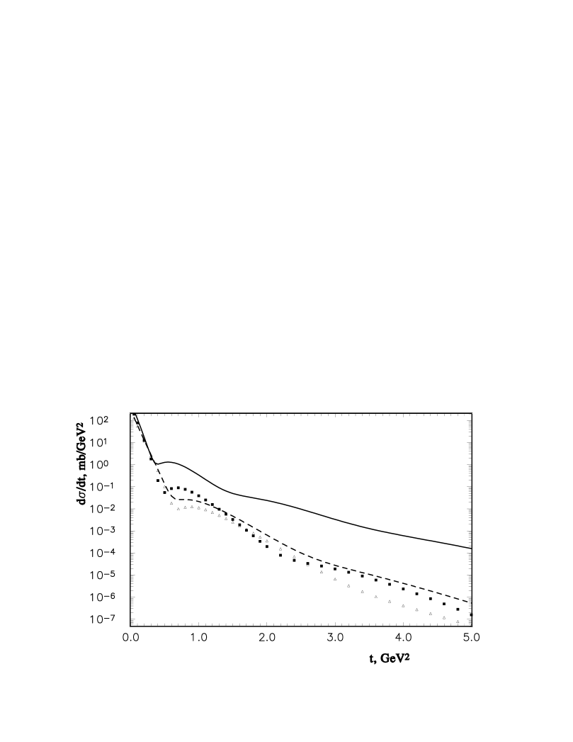
Figure 13: Predictions of the DD (solid and dashed lines) and BSW models (triangles and full squares) for the differential cross section, at $\sqrt{s}=2\$TeV (dashed line and triangles) and $\sqrt{s}=10\$ TeV (solid line and full squares).

Let us note that a similar model, describing simultaneously different hadronic elastic cross sections, polarization and spin correlation effects was developed by Bourrely, Soffer and Wu [117, 118] (BSW). According to the physical picture of this model, each hadron appears as a black disk with a gray fringe, where the black disk radius increases as $\ln(s)$. It is interesting to compare the predictions of the BSW and DD models for the LHC energies. The result is shown in Fig. 13 and Table 6. The most important difference comes from the region $|t|>0.3$ GeV².

energy	model	$\sigma_{tot}$, mb	$\sigma_{el}$, mb	$\frac{\sigma_{el}}{\sigma_{tot}}$	$\rho(t=0)$	$\frac{d\sigma}{dt}|_{-t=1}\$mb/GeV2
2 TeV	DD	81	20.7	0.256 83	0.197	38.8
	BSW	76.1	17.9	0.235 82	0.128	11.2
10 TeV	DD	123	42.6	0.35	0.195	350
	BSW	98.4	26.8	0.27	0.122	38.6

Table 6: Comparison of the predictions from the DD and BSW models for two LHC energies.

Future experiments at the LHC will provide for an excellent possibility to test the theoretical argument on the peripheral rise of the eikonal phase at superhigh energies determined, in this approach, by the meson-cloud effects.

6 Intermediate and Large $|t|$

The definition of the transition between “soft” and “hard” physics is rather ambiguous, although there are phenomena indicative of this transition. One is the slow-down of the shrinkage of the cone, already noticed at the ISR, and attributed to the hard scattering of the constituents of nucleons. It will manifest also in the change of the exponential decrease to a power fall-off in $|t|$. Furthermore, in this region the exponential decrease of the scattering amplitude will be gradually replaced by a power one. These effects have a simple interpretation within a Regge-pole model with nonlinear trajectories. As shown in a number of papers (see e.g. Refs. [57, 59]), logarithmic trajectories in the dual Regge-model [60, 55] can mimic hard scattering of point-like constituents and the transition from the soft interaction of the extended objects, like strings, to the hard scattering of point-like particles, governed by the quark counting rules and/or QCD.

Figure 14: Typical behavior of the slope of a logarithmic trajectory. Using Eq. (44), the slope $\alpha^{\prime}(t)$ decreases between $t=-1$ and $t=-10$ by about a factor 3. According to Eq. (43) the shrinkage of the slope is expected to slow down by the same rate.

A particularly simple expression for the slope of the diffraction cone, illustrating the aforesaid phenomena, follows from the geometrical properties of the geometrical model (see Eq. 24 and Ref. [132]):

$$B(s,t)=k\alpha^{\prime}(t)\sigma_{t}(s),$$ (43)

where $k$ is a parameter and $\alpha^{\prime}(t)$ is the slope of the logarithmic Pomeron trajectory given by Eq. (3). By choosing $\gamma=1$ and $\beta=0.3$, we get from Eq. (3)

$$\alpha^{\prime}(t)=\frac{0.3}{1-0.3t}.$$ (44)

The slope $\alpha^{\prime}(t)$ given by Eq. (44) is shown in Fig. 14. The logarithmic trajectory (3) (or, similarly, (4)) mimics also the transition from the exponential decrease of the scattering amplitude in $t$ (soft physics) to a power one, according to

$$A(s,t)\sim e^{[b\alpha(t)]}s^{\alpha(t)}\sim e^{-[b+\ln(s)]\ln(-t)}.$$ (45)

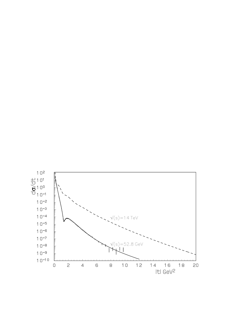
Figure 15: Predictions of the DD model for the differential cross section at $\sqrt{s}=52\$GeV (solid line) and at $\sqrt{s}=14\$TeV (dashed line) [88, 89]

.

Note that in this region the ratio $|t|/s$ is much smaller (tends to zero) than at the ISR energies. The new information obtained in this region (small angles and large $t$) will give the possibility to determine whether perturbative QCD works here. The logarithmic regime of the trajectory in the above Regge-pole model with the resulting power-like behavior in this kinematical region provides a link with the quark-parton model and, eventually, with the perturbative regime of QCD. However this transition is much more complicated, involves a rearrangement of the dynamics, that can be treated e.g. in the dual model of Ref. [59].

The valence $qq$ scattering is assumed to be due to a color singlet amplitude behaving as $s/t$, so that $d\sigma_{qq}/dt\sim t^{-2}$. For large $|t|$, this leads to a power-like behavior [133]: $d\sigma/dt\sim t^{-10}$, which corresponds to the dimensional counting rules [134, 135]. The perturbative QCD behavior can be preceded by a transition regime $d\sigma/dt\sim t^{-8}$.

Different models of “hard” scattering, with power-like scattering amplitudes obeying scaling, exist in the literature. For example, in a quark-diquark model of the nucleon [136], the introduction of the transverse distance $1/\sqrt{|t|}$ between the colliding valence quarks gives an additional degree of freedom.

Hard scattering and the power-low behavior of the cross sections by itself is an important issue of the strong interaction dynamics, which, however goes beyond the scope of the present paper. In large-$t$ elastic $pp$ scattering at the LHC one will enter only the transition region between the “soft” (exponential) and “hard” power-like behavior of the cross section.

Contrary to Eq. (45), that predicts the decrease of the differential cross section in this region, some models lead to an increasing elastic differential cross section at large momentum transfer. For example, the DD model [88, 89] describes the elastic differential cross section not only at small $|t|$, but also up to large $|t|\sim 10\$GeV² at the ISR (see Fig. 15). Note that the experimental data show that, up to the TeV-region, the differential cross section has a weak energy dependence at large $t$. This effect should be better understood, since in the TeV-region a change of the regime might occur, as Fig. 15 seems to indicate.

7 Black disc limit at the LHC?

There is general consensus on the hypothesis that with increasing energy nucleons are becoming blacker, edgier and larger (BEL effect). Since the details depend on model calculations and their extrapolations beyond the energies of present accelerators, the onset and consequences of BEL effect also differ. Of interest is the possibility that at the LHC the nucleons will reach the black disc limit (BDL) with measurable effects. If or when the black limit will be reached (at the LHC?) two cases, connected with the use of the $s-$channel unitarity, are possible. According to the first option, the BDL is identical to the unitarity limit, absolute for the central opacity of the nucleon. According to the second option (an alternative solution of the unitarity equation, which will be illustrated below), the unitarity limit is well beyond the BDL, leaving space for a further increase with energy of the central “overlap function” (or impact parameter amplitude). In this approach, the nucleon, after having reached the BDL and tending to the unitarity limit, will gradually become more transparent. Below we present both options and their observable consequences.

7.1 Definitions

The onset of “saturation”, wherever it occurs, can hardly be seen directly from the data, since the behaviour of the real part of the amplitude is at best known in the nearly forward direction only, while for the rest it can be only modelled. The expected approach to the BDL depends both on the model for the scattering amplitude which is used and on the procedure of unitarization. Numerical estimates based on particular model calculations are presented in the two subsequent subsections.

To start with, let us remind the general definitions and notations. Unitarity in the impact parameter $b$ representation reads

$$\Im{h(s,b)}=\big{|}h(s,b)\big{|}^{2}+G(s,b).$$ (46)

Here $h(s,b)$ is the elastic scattering amplitude at the center of mass energy $\sqrt{s}$, $\Im h(s,b)$ is usually called the “profile function”, representing the hadron opacity and $G(s,b)$, called the “inelastic overlap function”, is the sum over all inelastic channel contributions. Integrated over ${b}$, Eq. (46) reduces to a simple relation between total, elastic and inelastic cross sections:

$$\sigma_{tot}(s)=\sigma_{el}(s)+\sigma_{in}(s).$$

Eq. (46) imposes the absolute limit

$$0\leq\big{|}h(s,b)\big{|}^{2}\leq\Im h(s,b)\leq 1,$$ (47)

while the so-called black disc limit

$$\sigma_{el}(s)=\sigma_{in}(s)={1\over 2}\sigma_{tot}(s)$$

or

$$\Im h(s,b)=\frac{1}{2}$$ (48)

is a particular realization of the optical model, namely it corresponds to the maximal absorption within the eikonal unitarization, when the scattering amplitude is approximated as

$$h(s,b)={i\over 2}\left(1-\rm{exp}\left[i\ \omega(s,b)\right]\right),$$ (49)

with a purely imaginary eikonal $\omega(s,b)$.

The solutions of the unitarity equation (46), with $\Re h(s,b)=0$, are

$$h(s,b)={1\over 2}\left[1\pm\sqrt{1-4G(s,b)}\right].$$ (50)

The solution with the minus sign in front of the square root describes the eikonal unitarization. The other one, that with the plus sign in front of the square root, is known within the so-called $U$-matrix approach [137, 138, 139, 132], where the unitarized amplitude has the form of a ratio rather than of an exponential, typical of the eikonal approach. It is written as

$$h(s,b)={{U(s,b)}\over{1-i\ U(s,b)}},$$ (51)

where $U$ is the input Born term, the analogue of the eikonal $\omega$ in Eq. (49). The connection between the two forms was discussed in recent papers [140, 141].

In the $U$-matrix approach, the scattering amplitude $h(s,b)$ may exceed the black disc limit as the energy increases. The transition from a (central) black disc to a (peripheral) black ring, surrounding a gray disc, for the inelastic overlap function in the impact parameter space corresponds to the transition from shadowing to antishadowing [139]. We shall present a particular realization of this regime.

The impact parameter amplitude $h(s,b)$ can be calculated either directly from the data, as it was done e.g. in Ref. [142] (where, however, the real part of the amplitude was neglected) or by using a particular model that fits the data sufficiently well. We consider three representative examples, namely the Donnachie-Landshoff (DL) model [1, 2, 143, 144, 145, 146], the DP model [26, 27, 132] and the DD model [125, 128, 129, 114].

7.2 The “Born term”

The Donnachie-Landshoff model [1, 2, 143, 144, 145, 146] is very popular for its simplicity. Essentially, it means the following four-parametric empirical formula to fit all total hadronic cross sections

$$\sigma_{tot}=X\ s^{\delta}+Y\ s^{\delta_{r}},$$ (52)

where two of the parameters, namely $\delta=\alpha_{P}(0)-1\approx 0.08$, and $\delta_{r}$, which is negative, are universal. The violation of the Froissart-Martin (FM) bound,

$$\sigma_{tot}(s)<C\ (\ln{s})^{2},\ \ \ \quad C=60\ {\rm mb},$$ (53)

inherent to this model, is rather an aesthetic than a practical defect.

The $t$ dependence in the DL model is usually chosen [143, 144, 145, 146] in the form close to the dipole Pomeron form factor. For the present purposes a simple exponential residue in the Pomeron amplitude will do as well, with the signature included:

$$A(s,t)=-\ N\left(-i{s\over s_{dl}}\right)^{\alpha(t)}e^{Bt}\ ,$$ (54)

where $\alpha(t)=\alpha_{P}(0)+\alpha^{\prime}\ t$ is the Pomeron trajectory and $N$ is a dimensionless normalization factor related to the total cross section at $s=s_{dl}$ by the optical theorem:

$$N={s_{dl}\over 4\pi\sin{{\pi\over 2}\alpha_{P}(0)}}\sigma_{tot}(s=s_{dl})\ .$$ (55)

According to fits of Ref. [143, 144, 145, 146] one has $s_{dl}=1$ GeV², $\alpha_{P}(0)=1.08$, $\alpha^{\prime}=0.25$ GeV^-2, and $X=21.70$ mb (see (Eq. 52)) and thus $N=4.44$. By puting

$${d\sigma(s,t)\over dt}\ ={d\sigma(s,t=0)\over dt}\ e^{B_{exp}(s)\ t}$$ (56)

and choosing the CDF or E410 results for the slope $B_{exp}$ at the Tevatron energy, we obtain $B=B_{exp}(s)/2-\alpha^{\prime}\ln({{s/s_{dl}}})=4.75$ GeV^-2.

In the DP model [132], factorizable at asymptotically high energies, logarithmically rising cross sections are produced at the Pomeron intercept equal to one, so that the DP model does not conflict with the FM bound. While data on total cross section are compatible with a logarithmic rise (according to the DP model), the ratio $\sigma_{el}/\sigma_{tot}$ is found (see Ref. [132] for details) for $\delta=0$ to be a monotonically decreasing function of the energy for any physical value of the parameters. The experimentally observed rise of this ratio can be achieved only for $\delta>0$ and thus requires the introduction of a supercritical Pomeron, with $\alpha(0)>1$. As a result, the rise of the total cross section is driven and shared by the dipole Pomeron and the “supercritical” intercept. The parameter $\delta=\alpha_{P}(0)-1$ in the supercritical DP model is nearly half that of the DL model, making it safer from the point of view of the unitarity bounds. Generally speaking, the closer the input to the unitarized output, the better the convergence of the unitarization procedure.

Let us remind that, apart from the conservative FM bound, any model should satisfy also $s$-channel unitarity. We demonstrate below that both the DL and DP models are well below this limit and will remain so for long time, in particular at LHC. Let us remind that the DL and the DP model are close numerically, although they are different conceptually and consequently their extrapolations to superhigh energies will differ as well.

The elastic scattering amplitude corresponding to the exchange of a dipole Pomeron reads

$$\begin{array}[]{rcl}P(s,t)={d\over{d\alpha}}\left[{\rm e}^{-i\pi\alpha/2}G(\alpha)(\frac{s}{s_{0}})^{\alpha}\right]\\ =&{\rm e}^{-i\pi\alpha/2}(\frac{s}{s_{0}})^{\alpha}\big{[}G^{\prime}(\alpha)+(L-i\pi/2)G(\alpha)\big{]},\end{array}$$ (57)

where $L\equiv$ln${\frac{s}{s_{0}}}$ and $\alpha\equiv\alpha_{P}(t)$ is the Pomeron trajectory.

By setting $G^{\prime}(\alpha)=-a{\rm e}^{b_{p}(\alpha-1)},$ Eq. (57) can be rewritten in the geometrical form discussed in Subsection 5.1, (see Eq. (24)).

In Table 7 we quote the numerical values of the parameters of the DP model fitted in Ref. [26, 27] to the data on proton-proton and proton-antiproton elastic scattering:

$$\sigma_{tot}(s)={4\pi\over s}\Im A(s,0)\ ,\ \rho(s)={\Re A(s,0)\over{\Im A(s,0)}}\quad;\qquad 4\;({\rm GeV})\leq\sqrt{s}\leq 1800\;({\rm GeV})$$ (58)

as well as the differential cross-section

$${d\sigma(s,t)\over dt}\ =\ {\pi\over s^{2}}\left|A(s,t)\right|^{2},23.5\;({\rm GeV})\leq\sqrt{s}\leq 630\;({\rm GeV}),0\;({\rm GeV^{2}})\leq|t|\leq 6\;({\rm GeV}^{2})\;.$$ (59)

In that fit, apart from the Pomeron, the Odderon and two subleading trajectories $\omega$ and $f$ were also included. Here, for simplicity and clarity we consider only the dominant term at high energy due to the Pomeron exchange with the parameters fitted in Ref. [26, 27].

$a$	$b_{p}$	$\alpha_{P}(0)$	$\alpha^{\prime}$(GeV-2)	$\epsilon$	$s_{0}$(GeV2)
355.6	10.76	1.0356	0.377	0.0109	100.0

Table 7: Values of the parameters of the DP model, Subsections 5.1 and 7.2, found in Ref. [26, 27].

We use the above set of parameters to calculate the impact parameter amplitude.

7.3 Impact parameter representation, the black disc limit
and unitarity

The elastic amplitude in the impact parameter representation in our normalization is

$$h(s,b)\ =\ {1\over 2s}\int^{\infty}_{0}dq\ qJ_{0}(bq)A(s,-q^{2}),~{}~{}~{}~{}\quad\ q=\sqrt{-t}\ ,$$ (60)

expressed in tems of the Bessel function $J_{0}$.

The impact parameter representation for linear trajectories is calculable explicitly for the DP model using Eq. (57). We have

$$h(s,b)\ =i\ g_{0}\ \big{[}e^{r_{1}^{2}\delta}\ e^{-{b^{2}/4R_{1}^{2}}}\ -\ \epsilon\ e^{r_{2}^{2}\delta}\ e^{-{b^{2}/4R_{2}^{2}}}\big{]}\ ,$$ (61)

where the functions $r_{i}^{2}\equiv r_{i}^{2}(s)(i=1,2)$ have been introduced in the Subsection 5.1 and

$$R_{i}^{2}=\alpha^{\prime}r_{i}^{2}~{},\ \ \ g_{0}={a\over 4b_{p}\alpha^{\prime}s_{0}}\ .$$ (62)

Asymptotically (i.e. when $L\gg b_{p}$, which implies $\sqrt{s}\gg 2.$ TeV, with the parameters of Table 7) we get

$$h(s,b)\rightarrow i\ g(s)\ (1-\epsilon)\ e^{-{b^{2}\over 4R^{2}}},\ \ s\to\infty,$$ (63)

where

$$R^{2}=\alpha^{\prime}L~{},\ \ \ \ g(s)=g_{0}\left({s\over s_{0}}\right)^{\delta}\ .$$ (64)

To illustrate the effect coming from $s$-channel unitarity, in Ref. [148, 149] a family of curves showing the imaginary part of the amplitude in the impact parameter-representation as well as the inelastic overlap function $G(s,b)$ calculated from Eq. (46) at various energies, was displayed.

Our confidence in the extrapolation of $\Im h(s,b)$ to the highest energies rests partly on the good agreement of our (non fitted) results with the experimental analysis of the central opacity of the nucleon (see Table 8).

$\sqrt{s}$	53 GeV	546 GeV	1800 GeV
exp	0.36	$0.420\pm 0.004$	$0.492\pm 0.008$
th	0.36	0.424	0.461

Table 8: Central opacity of the nucleon $\Im h(s,0)$ calculated at ISR, SPS and Tevatron energies compared with experimental results.

It is important to note that the unitarity bound $1$ for $\Im h(s,b)$ will not be reached at the LHC energy, while the black disc limit $1/2$ will be slightly exceeded, the central opacity of the nucleon being $\Im{\rm m}h(s,0)=0.54$.

The black disc limit is reached at $\sqrt{s}\sim 2$ TeV, where the overlap function reaches its maximum value $1/4$. This energy corresponds to the appearance of the antishadow mode in agreement with the general considerations in Ref. [139]. Notice that while $\Im h(s,b)$ remains central all the way, $G(s,b)$ is getting more peripheral as the energy increases starting from the the value of Tevatron. For example at $\sqrt{s}=14$ TeV, the central region of the antishadowing mode, obtained from the $U$ matrix unitarization, below $b\sim 0.4$ fm is discernible from the peripheral region of shadowing scattering beyond $b\sim 0.4$ fm, where $G(s,b)={1/4}$. Consistently with the BEL effect the proton will tend to become more transparent at the center (in the sense of becoming a gray object surrounded by a black ring), i.e. it is expected to become gray, edgier and larger (GEL effect).

The $s$ channel unitarity limit will not be endangered until extremely high energies ($10^{5}$ Gev for the DL model and $10^{6}$ GeV for the DP model), safe for any credible experiment. It is interesting to compare these limits with the one imposed by the FM bound: actually the Pomeron amplitude saturates the FM bound at $10^{27}$ GeV. As expected, the FM bound is even more conservative than that following from $s$-channel unitarity.

Now, we consider the unitarized amplitude according to the $U$-matrix prescription [137, 138, 132]

$$H(s,b)={h(s,b)\over{1-ih(s,b)}}~{},$$ (65)

with the Born term $h(s,b)$ calculated from Eq. (60) using Eq. (57).

An unescapable consequence of the unitarization is that, when calculating the observables, one should also replace the Born amplitude $A(s,t)$ with a unitarized amplitude $\widetilde{A}(s,t)$ defined as the inverse Fourier-Bessel transform of $h(s,b)$:

$$\widetilde{A}(s,t)\ =\ {2s}\int^{\infty}_{0}db\ bJ_{0}(b\sqrt{-t})H(s,b)\ .$$ (66)

Thus, the above picture may change since the parameters of the model should in principle be refitted under the unitarization procedure (this effect of changing the parameters was clearly demonstrated e.g. in Ref. [150]).

While the unitarity limit now is secured automatically (remind that $\Im h(s,0)$ is well below that limit even at the Born level in the TeV region), the behaviour of the elastic impact parameter amplitude after it has reached the black disc limit corresponds (see Ref. [139]) to the transition from shadowing to antishadowing. In other words, the proton (antiproton) after having reached its maximal blackness around $2$ TeV, will become gradually more transparent with increasing energies at its center. It follows from the presented model that, in getting edgier and larger, the proton, after reaching its maximal blackness, will tend to be more transparent (GEL effect), i.e. a gray disc surrounded by a black ring will gradually develop beyond the Tevatron energy range. The transition from shadowing to a new, antishadowing scattering mode is expected to occur at the LHC.

To conclude, we stress once more that both the data and relevant models at present energies are well below the $s$-channel unitarity limit. Deviations due to the diversity of realistic models may result in discrepancies concerning $\Im{h(s,0)}$ of at most $10\%$, while its value at 2 TeV is still half that of the unitarity limit, so there is no reason to worry about it. Opposite statements may result from the confusion with normalization. Therefore, the model amplitudes at the Born level may still be quite interesting and efficient in analyzing the data at energies of present accelerator and giving some predictions beyond. The question, which model is closer to reality and meets better the requirements of the fundamental theory remains of course topical.

7.4 Saturation at the LHC (in the DD model)

The effect of the Black Disc Limit (BDL) saturation can be observed in the change of the $t$-dependence of the slope $B$ and of the ratio $\rho$ beginning from approximately $\sqrt{s}=2\div 6\$TeV and tending to enhance at $\sqrt{s}=14\$TeV [90]. Such a saturation effect was studied in the framework of the DD model.

In Refs. [90, 151] the BDL is determined by account of a hard Pomeron. The model predicts the increase with $|t|$ of the slope $B(t)$ at small $t$ and energies typical of the LHC, as shown in Fig. 16, right panel. In the same Figure, left panel, it is shown that saturation of the BDL substantially modifies the $t$-dependence of the ratio $\rho(s,t)$ (see, also, Table 9).

${\rho}\ (\sqrt{s}=14\$TeV, t)
$t=0\$ GeV 2		$t=-0.1\$ GeV 2
DD [88, 89]	Soft and hard Pomeron [90]	DD	Soft and hard Pomeron
$0.19$	$0.24$	$0.08$	0.05

Table 9: The effect of saturation on the ratio $\rho(t)$ as predicted in Refs. [88, 89], [90].

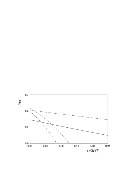
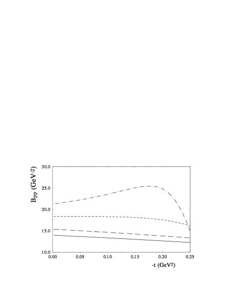
Figure 16: Left panel: The ratio of the real to the imaginary part of the amplitude as a function of $t$, for the bare and the saturated amplitudes at various energies: 100 GeV (solid line), 500 GeV (long dashes), 5 TeV (short dashes) and 14 TeV (dash-dotted curve). Right panel: The slope of the elastic differential cross section as a function of $t$, for the bare and saturated amplitudes at various energies: $100$ GeV (solid line), $500$ GeV (long dashes), 5 TeV (short dashes) and 14 TeV (dash-dotted curve).

In fact, saturation naturally predicts a small increase of the slope $B(t)$ with $t$ at small $t$. To understand this phenomenon, let us take a simple black disk form with a sharp edge at radius $R$. The relevant scattering amplitude can then be written as

$$A(s,t=0)\ \sim\ \frac{J_{1}(\sqrt{-t}R)}{\sqrt{-t}R}\ .$$

In this model the slope of the differential cross section at small momentum transfer behaves as

$$B_{BDL}\sim\frac{R^{2}}{4}+\left(\frac{R^{4}}{32}\right)|t|.$$ (67)

Hence the slope grows with increasing $|t|$ at small momentum transfer, as one can see in Fig. 16. It is interesting that two quite different models lead practically to the same result.

Saturation is usually attibuted to the growing gluon density at small $x$. This phenomeonon is important at relatively large impact parameters, where the role of non-perturbative effects [152], due to confinement, is not clear. On the other hand, the BDL-saturation is generally connected with the small impact parameter region. Scrutinizing the small $|t|$ region and looking for possible saturation effects there [153] is of great interest for future LHC measurements.

8 Summary and outlooks

In the present paper we concentrated mainly on elastic scattering and total cross sections. It should be remembered that the elastic scattering amplitude is the central, in a sense, basic object of the theory, therefore its knowledge is essential for the further progress in understanding strong interactions. Furthermore, elastic scattering, by unitarity (see, e.g. Sec. 7), is directly connected to inelastic processes.

The LHC facilities provide a unique experimental environment where one can test properties of the Pomeranchuk trajectory. Let us remind the open questions and problems that can be addressed both theoretically and experimentally:

$\bullet$ The Pomeron intercept. From perturbative QCD the value of about $\alpha(0)\approx 1.25$ follows [17, 18, 19, 20]. It should be remembered, as often stressed by the authors of the BFKL equation, that this value should not be confronted with the data prior the unitarization of the amplitude (that will lower the rate of increase of the total cross section). A complete unitarization procedure, however, is difficult to be realized. In any case, experimental measurement of the total cross section will shed new light on the value of the Pomeron intercept.

$\bullet$ Similar arguments concern the slope of the trajectory, which, because of its non-linear nature, is $t$-dependent. Hence it is important to explore the small $|t|$ region of the elastic differential cross section.

$\bullet$ By parameterizing the diffraction cone by the method of overlapping bins, the fine structure of the cone (or that of the Pomeron) will be detected (Sec. 3).

$\bullet$ Perturbative QCD predicts logarithmic asymptotics for the Pomeron trajectory, as in Eq. (3). This basic result of QCD is often ignored. At the LHC, the onset of, or approach to the logarithmic behavior of the Pomeron trajectory should be visible.

$\bullet$ The “QCD Pomeron” [17, 18, 19, 20] implies an infinite number of poles or a moving cut, which are difficult to be realized phenomenologically. In a simplified version, they can be approximated as a sum of two poles with different intercepts.

$\bullet$ The shape and the depth of the expected diffractive minimum and its ratio to the height of the second maximum are extremely informative (Sec. 5). The theoretical predictions here are not unique, but future data from LHC will narrow the margin for existing theoretical models.

$\bullet$ The expected transition from soft to hard physics will be revealed at the LHC. The determination of the $s$ dependence of the elastic cross section for $|t|>1$ GeV² will be very important for understanding the onset of the new, “hard” dynamics, replacing the “soft”, diffractive one.

$\bullet$ A basic characteristics of the strong interaction dynamics is the ratio $R(s)=\sigma_{el}/\sigma_{t}$, reflecting the intensity of particle production and/or the realization of a particular unitarization scheme. In the past, $R(s)$ was changing unpredictably: from the (seemingly asymptotic) constant in the ISR energy region, suggesting geometrical scaling, to a subsequent indefinite rise. Will this trend continue or a ”new asymptotic” plateau is expected at the LHC?

9 Acknowledgements

We thank Mario Deile, Alan Martin, Marcio Jose Menon, Francesco Paccanoni, Vladimir Petrov, Jacques Soffer and Serguey Troshin for useful remarks. L.J. and O.S. are grateful to the Department of Theoretical Physics of the University of Torino and the Department of Physics of the University of Calabria and the Istituto Nazionale di Fisica Nucleare - Sezione di Torino and Gruppo Collegato di Cosenza, where part of this work was done, for their warm hospitality and support. R.O. wants to express his gratitude to the Academy of Finland for support. A.P. and R.F. acknowledge partial support by the Italian Ministry of University and Research.

References

- [1] P.V. Landshoff,The Total cross-section at the LHC Lectures at School on QCD, Calabria, July 2007, hep-ph/0709.0395.
- [2] P.V. Landshoff,The Total cross-section at the LHC Proceedings of the 11th International Conference on Elastic and Diffractive Scattering: Towards High Energy Frontiers: The 20th Anniversary of the Blois Workshops, Chateau de Blois, Blois, France, 15-20 May 2005.
- [3] R. Orava, Forward Physics at the LHC, An invited talk at the 4-th Nordic LHC Physics Workshop, Stockholm 22-24 November 2001.
- [4] R. Orava, Diffraction at the LHC, Workshop on Diffractive Physics, LISHEP 2002, Rio de Janeiro, Brazil, 4-6 February 2002.
- [5] J. Lämsä and R. Orava, and J. Kallipuska, J. Lämsä, T. Maki, N. Marola, R. Orava, K. Ostanberg, M. Ottela, HIP-2003-11/EXP (2003).
- [6] A. DeRoeck, V.A. Khoze, A.D. Martin, R. Orava, and M.G. Ryskin, Eur. Phys. J. C25, 391 (2002).
- [7] M.G. Albrow at al. (Fp420 Collaboration), The Fp420 R&D Project: HIggs and New Physics with forward protons at the LHC, arXiv:0806.0302 (hep-ex).
- [8] V. Barone and E. Predazzi, High-Energy Particle Diffraction, Springer-Verlag, Berlin, (2002).
- [9] M. Bertini, P. Desgrolard, Yu.M. Ilyin, Int’l J. Phys. (Lahore) 1, 45 (1995).
- [10] L.L. Jenkovszky, Phys. Part. Nucl. 34, 619 (2003); Fiz. Elem. Chast. Atom. Yadra 34, 1196 (2003).
- [11] M. Bertini, M. Giffon, and E. Predazzi, Phys. Lett. B349, 561 (1995).
- [12] M. Bertini, M. Giffon, and E. Predazzi, Polarized Structure Functions from Deep Inelastic Scattering, Proceedings of the VI-th International Conference on Elastic and Diffractive Scattering, Blois, France, 20-24 June, 1995.
- [13] M. Bertini, M. Giffon, and E. Predazzi, Do We Really Need More than One Pomeron?, Proceedings of the VI-th International Conference on Elastic and Diffractive Scattering, Blois, France, 20-24 June, 1995.
- [14] M. Bertini et al. Rivista Nuovo Cim. 19, 1 (1996).
- [15] Rohina M. Godbole, Agnes Grau, Rohat Hedge, Giulia Pancheri, Yogi Srivastava, Theoretical expectations for total cross sections at the large hadron collider, Pranama 66, 657 (2006).
- [16] B.Z. Kopeliovich, I.K. Potashnikova, B. Povh, and E. Predazzi, Phys. Rev. Lett. 85, 507 (2000).
- [17] Y.Y. Balitsky and L.N. Lipatov, Sov. J. Nucl. Phys. 28, 822 (1978).
- [18] E.A. Kuraev, L.N. Lipatov, and V.S. Fadin, Sov. J. JETP 44, 443 (1976); Sov. J. JETP 45, 199 (1977);.
- [19] V.S. Fadin, L.N. Lipatov, Phys. Lett. B 429, 127 (1998).
- [20] M. Ciafaloni, G. Camici, Phys. Lett. B 430, 349 (1998).
- [21] A. Donnachie and P.V. Landshoff, Nucl. Phys. B244, 737 (1984).
- [22] R. Avila, P. Gauron, and B. Nicolescu, Eur. Phys. J. C49, 581 (2007).
- [23] L.L. Jenkovszky, B.V. Struminsky, and A.N. Shelkovenko, Yad. Fizika (Engl. Transl.: Sov. J. Nucl. Phys. 12, 2732 (1987).
- [24] L.L. Jenkovszky, B.V. Struminsky, and A.N. Shelkovenko, Z. Phys. C36, 495 (1987).
- [25] L.L. Jenkovszky, B.V. Struminsky, and A.N. Shelkovenko, Pisma JETP (Engl. Transl.: JETP Letters) 47, 288 (1998).
- [26] R.J.M. Covolan et al., Z. Phys. C58, 109 (1993).
- [27] P. Desgrolard, M. Giffon, and L.L. Jenkovszky, Z. Phys. C55, 637 (1992).
- [28] P. Gauron, L.N. Lipatov, and B. Nicolescu, Phys. Lett. B260, 407 (1991).
- [29] E. Predazzi, Odd-Parity Effects in Diffraction, Proceedings of DIS-96, May 1996, Rome, G. D’Agostini and A. Nigro Editors, World Scientific, 410.
- [30] M. Giffon, E. Predazzi, and A. Samokhin, Phys. Lett. B375, 315 (1996).
- [31] M. Giffon, E. Predazzi, and A. Samokhin, Possible C-Odd Effects in High-Energy and Elastic Scattering at , Proceedings of the 12th International Conference on High-energy Physics (HADRONS 96), Novy Svet 9-16 June 1996, Hadrons-96’, Kiev, 1996, p, 199.
- [32] M. Giffon, E. Predazzi, and A. Samokhin, C-Odd Effects in the Diffractive Domain, proceedings of the 28th to the International Conference on High-energy Physics (ICHEP 96), Warsaw, 25-31 July 1996, ICHEP’96’, Warsaw, 1996, p. 613.
- [33] A.P. Contogouris et al. Phys. Lett. B298, 432 (1993).
- [34] A. Breakstone et al. Phys. Rev. Lett. 54, 2180 (1985).
- [35] S. Erhan et al. Phys. Lett. B152, 131 (1985).
- [36] A. Degasperis and E. Predazzi, Nuovo Cim. A65, 764 (1970).
- [37] H. Fleming and E. Predazzi, Nuovo Cim. Lett. 4, 556 (1970).
- [38] A.N. Vall, L.L. Jenkovszky, and B.V. Struminsky, Sov. J. of Particles and Nuclei, 19, 77 (1988).
- [39] G. Cohen-Tannoudju et al. Lett. Nuovo Cim. 5, 957 (1972).
- [40] A. Anselm and V. Gribov, Phys. Lett. B40, 487 (1972).
- [41] V.A. Khoze, A.D. Martin, and M.G. Ryskin, Eur. Phys. J. C18, 167 (2000).
- [42] B.Z. Kopeliovich and A.V. Tarasov, Phys. Lett. B497, 44 (2001).
- [43] A.O. Barut and D.E. Zwanziger, Phys. Rev. 127, 974 (1962).
- [44] V.N. Gribov and Ya.I. Pomeranchuk, Nucl. Phys. 38, 516 (1962).
- [45] R. Taylor, Phys. Rev. 127, 974 (1962).
- [46] R. Oehme, presented at the Scottish Summer School 1963, Edited by R.G. Moorhousw et al. Edinbourgh (1964) p.129.
- [47] R. Fiore et al., Eur. Phys. J. A10, 217 (2001).
- [48] R. Fiore et al., Phys. Rev. D70 (2004) 054003.
- [49] M. Giffon, Y. Hama, and E. Predazzi, Z. Phys. C25, 129 (1984).
- [50] M. Giffon and E. Predazzi, Phys. Lett. B150, 317 (1985).
- [51] M. Giffon, R. Nahabetian, and E. Predazzi, Z. Phys. C36, 67 (1987).
- [52] M. Giffon, R.S. Nahabetian, and E. Predazzi, Phys. Lett. B205, 363 (1988).
- [53] A.I. Bugrij et al., Fortschritte Phys. 21, 427 (1973).
- [54] L.L. Jenkovszky, Fortschritte Phys. 34, 702 (1986).
- [55] L.L. Jenkovszky, Rivista Nuovo Cim. 10, 1 (1987).
- [56] M.M. Brisudova, L. Burakovsky, and T. Goldman, Phys. Rev. D61, 054013 (2000).
- [57] D.D. Coon et al., Phys. Rev. D18, 1154 (1978).
- [58] L.L. Jenkovszky and Z.E. Chikovani, Yad. Fiz. 30, 531 (1979).
- [59] R. Fiore, L.L. Jenkovszky, V.K. Magas, and F. Paccanoni, Phys. Rev. D60, 116003 (1999).
- [60] L. Jenkovszky, Nucl. Phys. B (Poc. Suppl.) 12, 317 (1990).
- [61] TOTEM Collaboration, TOTEM TDR, CERN-LHCC-2005-002 (2004); The numbers referring to the stage-1 ’pilot’ optics with m are based on preliminary TOTEM studies.
- [62] The TOTEM experiment at the CERN Large Hadron Collider. By TOTEM Collaboration (G. Anelli et al.), 2008, 112pp, Published in JINST 3:S08007, 2008.
- [63] V.A. Khoze (Durham), A.D. Martin (Durham), R. Orava (Helsinki), and M.G. Ryskin (St. Petersburg) Luminosity monitors at the LHC, Eur. Phys. J. C19, 313 (2001).
- [64] M. Albrow, A. De Roeck, V. Khoze, J. Lämsä, E. Norbeck, Y. Onel, R. Orava, and M.G. Ryskin, Forward physics with rapidity gaps at the LHC, to be published.
- [65] Forward physics and luminosity determination at LHC. Proceedings, Workshop, Helsinki, Finland, October 31-November 4, 2000. K. Huitu, (ed.), R. Orava, (ed.), S. Tapprogge, (ed.) (Helsinki Inst. of Phys. & Helsinki U.) , V. Khoze, (ed.) (Durham U.) . 2001. 226pp. Prepared for 1st Workshop on Forward Physics and Luminosity Determination at LHC, Helsinki, Finland, 31 Oct - 4 Nov 2000. Published in New Jersey, USA: World Scientific (2001) 226 p.
- [66] The FP420 R&D Project: Higgs and New Physics with forward protons at the LHC. By FP420 R&D Collaboration (M.G. Albrow et al.). FERMILAB-FN-0825-E, Jun 2008. 176pp. Temporary entry e-Print: arXiv:0806.0302 [hep-ex].
- [67] R. Orava, Forward Physics Measurements at the LHC, Proceedings of “Diffraction 2006: 4th International Workshop on Diffraction in High-energy Physics”, Adamantas, Milos Island, 5-10 September 2006, PoS D IFF2006 (2006) 020.
- [68] A. De Roeck, V. A. Khoze, A. D. Martin, R. Orava and M. G. Ryskin, Eur. Phys. J. C 25, 391 (2002) [arXiv:hep-ph/0207042].
- [69] O.V. Selyugin, Phys. Lett. B333, 245 (1994).
- [70] V.A. Khoze, A.D. Martin, R. Orava, and M.G. Ryskin, Eur. Phys. J. C19, 313 (2001).
- [71] F. Ferro, TOTEM experiment at the LHC: status and program, Proceedings of “Diffraction 2006: 4th International Workshop on Diffraction in High-energy Physics”, Adamantas, Milos Island, 5-10 September 2006, PoS D IFF2006 (2006) 019.
- [72] M. Deile, Total Cross-Section Measurement and Diffractive Scattering with TOTEM, Proceedings of the 12-th Blois conference, Hamburg, 21-25 May 2007, J. Bartels et al. editors, arXiv:0712.3633 [hep-ph].
- [73] C. Sbarra, Elastic scattering, total cross section and luminocity measurements with ATLAS, Proceedings of the 12-th Blois conference, Hamburg, 21-25 May 2007, J. Bartels et al. editors, arXiv:0712.3633 [hep-ph].
- [74] P. Gauron, B. Nicolescu, and O.V. Selyugin, Phys. Lett, B629, 83 (2005).
- [75] Christophe Royon, Luminosity measurements and diffractive physics in ATLAS, Proceedings of “Diffraction 2006: 4th International Workshop on Diffraction in High-energy Physics”, Adamantas, Milos Island, 5-10 September 2006, PoS DIFF2006 (2006) 021.
- [76] H. Stenzel, ATL-LUM-PUB-2007-001.
- [77] V. Kundrat, M. Lokajicek, and I. Vrkoc, Phys. Lett. B 656 (2007) 182.
- [78] G.B. West and D.R. Yennie, Phys. Rev. 172, 1413 (1968).
- [79] R. Schicker, Low mass diffraction system at the LHC, Proceedings of “New Trends in HEP”, Yalta, Ukraine, sep 15-22, 2007; hep-ph/0801.4890;
- [80] R. Schicker, The ALICE detector and trigger strategy for diffractive and electromagnetic processes, arXiv:0807.1472v1 [physics.ins-det], 9 July 2008.
- [81] R. Schicker, In the Proceedings of Diffraction2008 conference, Le Londe-les-Maures, arXiv:hep-exp/0812.3123.
- [82] J.R. Cudell, A. Lengyel, E. Martynov, and O.V. Selyugin, The soft and the hard pomerons: elastic scattering and unitarisation, Proceedings of the 12-th Blois conference, Hamburg, 21-25 May 2007, J. Bartels et al. editors, arXiv:0712.3633 [hep-ph].
- [83] C. Bourrely, J. Soffer, and T.T. Wu, Nucl. Phys. B247, 15 (1984).
- [84] E. Gotsman, E. Levin, and U. Maor, and J.S. Miller, A QCD motivated model for soft interactons at high energies, arXiv:0805.2799 (hep-ph).
- [85] M.G. Ryskin, A.D. Martin and V.A. Khoze, Soft diffraction at the LHC: a partonic intrerpretaton, IPPP/07/66, DCPT/07/132 Preprint, 12 December 2007; arXiv: 0710.2494v3 [hep-ph].
- [86] J.R. Cudell et al. [COMPETE Collaboration], Phys. Rev. Lett. 89 (2002) 201801 .
- [87] B. Nicolescu, The Odderon at RHIC and LHC, Proceedings of the 12-th Blois conference, Hamburg, 21-25 May 2007, J. Bartels et al. editors, arXiv:0712.3633 [hep-ph].
- [88] S.V. Goloskokov, S.P. Kuleshov, and O.V. Selyugin, Particles & Nuclear, 18, 39 (1987).
- [89] S.V. Goloskokov, S.P. Kuleshov, and O.V. Selyugin, Zeitschrift Phys. C 50, 455 (1991).
- [90] J.R. Cudell and O.V. Selyugin, Saturation effects in diffractive scattering at LHC energies, Proceedings of 33rd International Conference on High Energy Physics (ICHEP 06), Moscow, Russia, 26 Jul - 2 Aug 2006.
- [91] V.A. Petrov, A.V. Prokudin, S.M. Troshin, and N.E. Tyurin, J. Phys. G27, 2225 (2001).
- [92] V.A. Petrov, E. Predazzi, and A. Prokudin, Eur. Phys. J. C28, 525 (2003).
- [93] M. M. Islam, R. J. Luddy, and A. V. Prokudin, Int. J. Mod. Phys. A21, 1 (2006).
- [94] H. Bethe, Ann. Phys. 3, 190 (1958).
- [95] R. Cahn, Z. Phys. C15, 253 (1982).
- [96] O.V. Selyugin, Mod. Phys. Lett. A9 (1994) 1207.
- [97] O.V. Selyugin, Mod. Phys. Lett. A14, 223 (1999).
- [98] O.V. Selyugin, Phys. Rev. D60, 074028 (1999).
- [99] O.V. Selyugin, Yad. Fiz. 55 , 841 (1992).
- [100] K. Goulianos, L.L. Jenkovszky, and B.V. Struminsky, Yad. Fizika (Engl. transl. Sov. J. Nucl. Phys.) 54, 573 (1991).
- [101] N.I. Starkov and V.A. Tsarev, Pisma Zh. Eksp. Teor. Fiz. 23, 403 (1976).
- [102] Yu.M. Antipov et al., Yad. Fiz. 35, 342 (1976).
- [103] N.P. Zotov, S.V. Rusakov, and V.A. Zarev, Particles and Nuclei 11, 1160 (1980).
- [104] S. V. Goloskokov, S. P. Kuleshov, and O. V. Selyugin, Spin effects in elastic hadron scattering at small and large angles, In “Protvino 1986, High energy spin physics, vol. 1” 107-118.
- [105] S.V. Goloskokov, S.P. Kuleshov, and O.V. Selyugin, Proceedings of V International Workshop “Problems of physics of high energies and quantum field theory”, Protvino, (1982), 189.
- [106] J. Kontros and A. Lengyel, Proceedings of International Workshop on High-energy Physics: Diffraction 95, Novy Svet, Ukraine, 6-11 Sep 1995, L.L. Jenkovsky editor, “Novy Svet 1995, Hadrons” (1995) 61.
- [107] O. Dumbrajs, J. Kontros and A. Lengyel, Heavy Ion Phys. 11, 13 (2000).
- [108] E.A. Kuraev, P. Ferro, and L. Trentadue, JINR preprint E2-97-95, Dubna 1995.
- [109] O.V. Selyugin, Oscillations of the hadronic amplitude at small transfer momenta, Proceedings of International Workshop on High-energy Physics: Diffraction 95, Novy Svet, Ukraine, 6-11 Sep 1995, G. Bugrij and L. Jenkovszky editors, p. 65.
- [110] P. Gauron, B. Nicolescu, and O.V. Selyugin, Phys. Lett. B397, 305 (1997).
- [111] D. J. Hudson, Statistics Lectures. 2. Maximum Likelihood And Least Squares Theory, (1964) CERN-64-18
- [112] A. Schiz et al. Phys. Rev. D24, 26 (1981).
- [113] G. Barbiellini et al. Phys. Lett. B39, 663 (1972).
- [114] S. V. Goloskokov, S. P. Kuleshov, and O. V. Selyugin, Sov. J. Nucl. Phys. 46, 329 (1988) [Yad. Fiz. 46, 597 (1987)].
- [115] T.T. Chou and C.N. Yang, Phys. Lett. B128, 457 (1983).
- [116] P. Desgrolard, M. Giffon, E. Predazzi, Zeitschrift Phys. C63, 241 (1994).
- [117] C. Bourrely, J. Soffer, and T.T. Wu, Phys. Rev. Lett. 54, 757 (1985).
- [118] C. Bourrely, J. Soffer, and T.T. Wu, Eur. Phys. J. C28, 97 (2003).
- [119] R.F. Avila and M.J. Menon, Eikonal zeros in the momentum transfer space from proton-proton scattering: An Empirical analysis, Eur. Phys. J. C 54, 555 (2008); hep-ph/0712.3398.
- [120] L.L. Jenkovszky and A.N. Wall, prepring ITP, Kiev, 1972; Czech J. Phys. B26, 447 (1976).
- [121] V. A. Petrov and A. V. Prokudin, Eur. Phys. J. C23, 135 (2002).
- [122] E. Predazzi, Annals of Physics 36, 228 (1966); ibid. Annals of Physics 36 , 250 (1966).
- [123] E. Predazzi and G. Soliani, Nuovo Cim. A2, 427 (1967).
- [124] K. Hinotani, H.A. Neal, E. Predazzi, and G. Walters, Nuovo Cim. A52, 363 (1979).
- [125] S.V. Goloskokov, S.P. Kuleshov, and O.V. Selyugin, Yad. Fiz. 31 (1980) 741; ibid. 34, 235 (1981); ibid. 46, 907 (1987).
- [126] M. M. Block, E. M. Gregores, F. Halzen, and G. Pancheri, Phys. Rev. D60, 054024 (1999).
- [127] P. Desgrolard, M. Giffon, E. Martynov, and E. Predazzi, Eur. Phys. J. C16, 499 (2000).
- [128] S.V. Goloskokov, S.P. Kuleshov, and O.V. Selyugin, Yad. Fiz. 35, 1530 (1982).
- [129] S.V. Goloskokov, S.P. Kuleshov, and O.V. Selyugin, Journal de Physique, C2 46, 239 (1984).
- [130] K.R. Schubert, In Landolt-Bronstein, New Series, v. 1/9a, (1979).
- [131] S.V. Goloskokov, S.P. Kuleshov, and O.V. Selyugin, Z. Phys. C50, 455 (1991).
- [132] A.N. Wall, L.L. Jenkovszky, and B.V. Struminsky, Sov. J. Nucl. Phys. 12, 901 (1987).
- [133] M. G. Sotiropoulos and G. Sterman, Nucl. Phys. B425, 489 (1994).
- [134] V.A. Matveev, R.M. Muradyan, A.N. Tavkhelidze, Lett. Nuovo Cim, 7, 719 (1973).
- [135] S. Brodsky and G. Farrar, Phys. Rev. Lett. 31, 1153 (1973).
- [136] M. Anselmino, E. Predazzi, S. Ekelin, S. Frederiksson, and D.B. Lichgtenberg, Rev. Mod. Phys. 65, 1199 (1993).
- [137] V.S. Savrin, N.E. Tyurin, and O.A. Khrustalev, Fiz. Elem. Chastic At. Yad. 7, 21 (1976) [Sov. J. Part. Nucl. 7, 77 (1976)].
- [138] S.M. Troshin and N.E. Tyurin, Phys. Lett. B316, 175 (1993).
- [139] S.M. Troshin and N.E. Tyurin, Int. J. of Physics, A22, 4437 (2007).
- [140] J.R. Cudell and O.V. Selugin, The soft and the hard pomerons: elastic scattering and unitarisation, [hep-ph/0710.5391].
- [141] S.M. Troshin, Comment on the “extended eikonal” unitarization, [hep-ph/0712.3359].
- [142] U. Amaldi and K.R. Schubert, Nucl. Phys. B166, 301 (1980).
- [143] A. Donnachie and P.V. Landshoff, Z. Phys. C2, 55 (1979).
- [144] A. Donnachie and P.V. Landshoff, Phys. Lett. B123, 345 (1983).
- [145] A. Donnachie and P.V. Landshoff, Nucl. Phys. B231, 189 (1983).
- [146] A. Donnachie and P.V. Landshoff, Nucl. Phys. B244, 322 (1984).
- [147] L. Jenkovszky and F. Paccanoni, Nuovo Cim. A 33, 329 (1976); ibid. 62, 133 (1981).
- [148] P. Desgrolard, L.L. Jenkovszky, and B.V. Struminsky, Yad. Fiz. 63, 962 (2000) (Engl. translation: Physics of Atominc Nuclei, 63, 891 (2000)).
- [149] P. Destrolard, L. Jenkovszky, B. Struminsky, EPJ C11, 145 (1999); hep-ph/9901437.
- [150] R. Covolan, K. Goulianos, and Montanha, Phys. Lett. B389, 176 (1996).
- [151] J.R. Cudell and O.V. Selyugin, Czech. J. Phys. 54, A441 (2004).
- [152] A. Kovner, Lectures at the XLV Cracow School of Theoretical Physics, Acta Phys. Polon. B36, 3551 (2005).
- [153] J.-R. Cudell, O. V. Selyugin, Phys. Lett. B 662, 417 (2008).