HHSMT Observations of the Venusian Mesospheric Temperature, Winds, and CO abundance around the MESSENGER Flyby

Abstract

We present submillimeter observations of ¹²CO J=3 -2 and J=2–1, and ¹³CO J = 2 -1 lines of the Venusian mesosphere and lower thermosphere with the Heinrich Hertz Submillimeter Telescope (HHSMT) taken around the second MESSENGER flyby of Venus on 5 June 2007. The observations cover a range of Venus solar elongations with different fractional disk illuminations. Preliminary results like temperature and CO abundance profiles are presented.

These data are part of a coordinated observational campaign in support of the ESA Venus Express mission. Furthermore, this study attempts to contribute to cross-calibrate space and ground-based observations, to constrain radiative transfer and retrieval algorithms for planetary atmospheres, and to a more thorough understanding of the global patters of circulation of the Venusian atmosphere.

, url]http://www.mps.mpg.de/homes/rengel/ ,

1 Introduction

NASA’s MESSENGER spacecraft swung by Venus for a second time on 6 June 2007 at 23:10 UTC on its way to Mercury. ESA’s Venus Express, on the other hand, is orbiting around Venus since 11 April 2006. Both spacecrafts carried out multi-point observations of the Venusian atmosphere on June 6 for several hours. Among the space-based observations, a world-wide Earth-based Venus Observation campaign from 23 May to 9 June 2007 (and later) was initiated to remotely observe the Venusian atmosphere. It contributes to the growing information on Venus’s atmospheric characteristics and complement the space-based data. Because Venus was close to its maximum eastern elongation during the time-frame of the ground-based observations, Venus was in a favorable position for observations of both its day and night sides.

The Venusian atmosphere is conventionally divided into three regions: the troposphere (below 70 km), the mesosphere (70 - 120 km), and the thermosphere (above 120 km). Studying the Venus’ mesosphere dynamics is of special interest because this region is characterized by the combination of two different wind regimes (a retrograde super-rotation and a sub-solar to anti-solar flow pattern), and affects both the chemical stability and the thermal structure of the entire atmosphere (Clancy et al., 2003). The principal feature of atmospheric general circulation is the super-rotation with typical wind velocities of 60–120 m s^-1. Mesospheric temperatures and CO mixing ratio experience global variations with time (Clancy and Muhleman, 1991), probably due to gravity wave breaking activity (Lellouch et al., 1994). Submillimeter spectral line observations play an important role in the investigation of the poorly constrained Venus mesosphere (it is the only technique to provide direct wind measurements in the mesosphere). Carbon monoxide (CO) is an important tracer in the atmosphere of Venus. Because its relatively strong transitions and the pressure-broadened lineshapes, it is the best measured trace component of the mesosphere (Kakar et al., 1976; Wilson et al., 1981).

This paper reports CO observations performed in June 2007 on the mesosphere of Venus as a part of the ground-based observing campaign in support of Venus Express and MESSENGER. We present some examples of the capabilities of these data by the use of radiative transfer and retrieval simulations: preliminary results of the absorption line Doppler wind velocities, and thermal and CO abundance vertical profiles.

2 Observations

CO Venus observations were made with the Heinrich Hertz Submillimeter Telescope (HHSMT), operated and owned by the Arizona Radio Observatory (ARO). The telescope is located at an elevation of 3178 m on Mount Graham, Arizona, and consists of a 10 m diameter primary with a nutating secondary. The observations were obtained on 8, 9, 10, 14 and 15 June from 18:30 to 0:30 UT. We used the 345 Superconductor-Insulator Superconductor (SIS) and the 2mmJT/1.3 mmJT ALMA receivers, operating respectively at 320–375 and 210–279 GHz to observe the CO J = 2 -1 (at a frequency of 230.538 GHz), ¹²CO J = 3 -2 (at 345.79 GHz), and ¹³CO J = 2–1 (at 220.398 GHz). The 345 SIS receiver was used in the single sideband mode with the signal frequency being placed once in the lower sideband (LSB) and another time in the upper sideband (USB), and the 2mmJT/1.3mmJT one only in the LSB. Here, the mixer itself is intrinsically a double sideband (DSB) mixer. The mixer is connected to the same input port at both USB and LSB, and then a DSB receiver can be used in two modes (to measure narrow-band signals contained entirely within one sideband, and to measure broadband (or continuum) sources whose spectrum covers both sidebands). System temperatures with the 345 GHz receiver were typically 1500 -2500 and 200 -500 K with the 2mmJT/1.3mmJT receiver. Seven different backends were used simultaneously: two 1 MHz Forbes filterbanks (FFBA and FFBB), two 970 MHz wide Acousto-Optical-Spectrometers (AOSA and AOSB), two filterbackends (FB2A and FB2B) filterbackends, and one 215 MHz CHIRP Transform spectrometer (CTS, resolution of $\sim$40 kHz) (Hartogh and Hartmann, 1990; Villanueva and Hartogh, 2006).

Observations were carried out during good atmospheric conditions (low water vapor), although on 10, 14, and 15 June it was partially cloudy. The observing mode was always dual beam switching. Pointing was checked every 2–3 h. The typical integration time per individual spectrum was around 4 min.

The angular diameter of Venus was 23.44^′′ at the beginning and 25.55^′′ at end of our campaign, respectively. The fraction of illumination for Venus was 49.95 and 45.68%, as seen by observer. Fig. 1 shows a synthetic image of the apparent disk of Venus that approximates the telescopic view of Venus as seen from the Earth at 8 June and 18:30 UT.

The CO J = 2 -1 line was mapped on 8 different beam positions on Venus disk, ¹²CO J = 3 -2 line on eight positions, and ¹³CO J = 2–1 line on one. The later one represents the first detection of this line on a planetary atmosphere at HHSMT. A summary of the observations carried out is provided in Table 1. Fig. 2 shows the mapping of the beam positions on Venus disk.

3 Data Analysis

The measured spectra were reduced with the CLASS software package of the Grenoble Astrophysics Group. A total of 36 spectra of Venus were taken.

The CTS is able to handle the strong continuum background from Venus due to its higher dynamical range larger than 30 dB. Because the retrieval of the temperature and CO distribution require clean spectra, this spectrometer is well suitable for our goals. Fig. 3 shows an example of the spectra morphology for ¹²CO J = 2 -1 line for different backends which we have used.

4 Observational Results

4.1 Qualitative wind measurements

The only method that provides wind measurements is the analysis of Doppler shifts of molecular lines. Spectral line differences with the East and West limb positions yields measurements of projected doppler velocities relative to the disk center (gives morning and afternoon zonal winds). Fig. 4 shows examples of the spectra of CO J = 2 -1 lines (Obs. no. 19, 25, and 28) at three different beam positions (5, 11, and 13). In this example the derived wind speed does not exceed 100 m s^-1. The Venus-HHSMT relative velocity at the time each scan is not computed here.

4.2 Thermal structure and CO Distribution

In order to retrieve the temperature profile and the CO distribution in the mesosphere, we have applied a retrieval technique described by C. D. Rodgers as optimal estimation (Rodgers, 1976). We used a radiative transfer code (Jarchow and Hartogh, 1995; Jarchow, 1998; Hartogh and Jarchow, 2004) which describes the physics of the radiative transfer through the atmosphere, to calculate the synthetic spectra which best fit the observed spectra. An a priori profile to be retrieved is required as initial input for the optimal estimation technique. Our atmospheric model consisted of 30 layers spanning the 40–120 km interval with a resolution of 2 km. Brightness temperatures were convolved with an assumed Gaussian beam. Below we present the retrieved temperature and CO vertical profiles taken in the center of the Venus disk obtained with our technique. At the other beam positions the results will be discussed elsewhere.

Examples (corresponding to Obs. nos. 5, 32, and 35 in Table 1) of fits to the ¹²CO J = 3 -2, CO J = 2 -1 and ¹³CO J = 2–1 lines in terms of temperature vertical profile are displayed in Figs. 5, 6, and 7, respectively. The spectrum of Obs. no. 35 presents signatures like periodic ripples in the baseline. Although the reasons of this anomaly is currently unknown (perhaps they are standing waves or an instrumental effect), we retrieved its thermal profile and CO distribution as a pure exercise. The baseline signatures may cause large retrieval errors, and we are aware that it requires further analysis.

Fig. 8 presents a comparison of the Obs. 5 temperature retrieval to the profiles from the SPICAV onboard Venus Express (Bertaux et al., 2007), Pioneer Venus (PV) descent probes (Seiff et al., 1980), to the OIR sounding measurements (Schofield and Taylor, 1983), and to the PV night probe (Seiff and Kirk, 1982). The extensive layer of warm air at altitudes 90–120 km detected by SPICAV (Bertaux et al., 2007) (interpreted as the result of adiabatic heating during air subsidence) seems to be also detected in the HHSMT profile at 90– to 100 km altitude, but the HHSMT peak shows a shorter temperature excess with respect to SPICAV measurements. The measurements with SPICAV for orbits 102–104 taken at altitude 4^∘ S, for orbits 95, 96, and 98 at 39^∘ N, and reported here at 0^∘ show the layer of warm air at altitudes of around 95, 100, and 97 km. In other words, if the adiabatic heating is a localized phenomena, the layer seems to move up (in altitude) with the latitude. Additional data at different latitudes are required. Furthermore, in other altitudes the HHSMT profile compares favorably to those returned by the previous measurements. Similar temperature profiles were also observed (Lellouch et al., 1994; Clancy et al., 2003). Furthermore, it was suggested that a 10-15 K increasing in the mesospheric temperatures occur over 1-30 day periods, and much large variations (20-40 K) over as yet undetermined timescales (Clancy et al., 2003).

5 Conclusion

• We have carried out several CO mm-wave line observations on different beam positions on Venus disk during June 2007.

• From spectra of ¹²CO J=2–1 and CO J=3–2 we retrieved well-resolved and accurate vertical profile of temperature and CO mixing ratio for the June 2007 mesosphere of Venus.

• The temperature peak detection reported here at 90-100 km seems to support the newly found of the extensive layer of warm air detected by SPICAV onboard Venus Express.

Despite the success of the analysis presented here, some points need further work. More accurate line-of-sight wind velocities on Venus will be determined, and gravitationally redshift corrected. A discussion about Venus circulation for this particular period of time will be given elsewhere later.

Table 1: Observation Parameters
Fig. 1: Synthetic image of Venus that approximates the telescopic view of Venus as seen from the Earth at 8 June and 18:30 UT. Dotted lines of longitude and latitude are shown on the surface in black, every 30 degrees, beginning at 0 degrees longitude and latitude.
Fig. 2: Black points show beam positions where the CO spectra were mapped on the Venus disk (for a 24^′′ disk diameter). Solid lines indicate the Venus’ equator and central meridian. Dashed circles indicate the approximate FWHM beam diameter. Left upper, right upper and left lower panels represent the positions for CO J = 2 -1, ¹²CO J = 3 -2, and ¹³CO J= 2–1 lines.
Fig. 3: Example of the spectra morphology for the ¹²CO J = 2 -1 line for different backends. Left center is the spectra taken with the CTS. Right upper, center, and lower panels show the spectra taken with AOS, FB2, and FFB backends. An integration time of 30 min was taken.
Fig. 4: East and west limb CO J=2–1 spectra (dot and short dash lines, respectively) compared to the disk center spectrum (solid line). Beam positions corresponds to 11 and 13. An upper limit wind velocity of 100 m s^-1 is estimated.
Fig. 5: Upper left panel shows the synthetic spectra solution for Obs. 5, and lower left panel, the difference between the observed and fitted spectra. Upper and lower middle panels indicate the retrieved temperature and CO abundance profiles derived from the spectrum. The gray lines show the initial profiles, and the horizontal lines are the error bars. Upper and lower right panels show the averaging kernels, i.e., the sensitivity of the retrieval.
Fig. 6: Solution for Obs. 32. See caption Fig. 5.
Fig. 7: Solution for Obs. 35. See caption Fig. 5.
Fig. 8: Temperature profile retrieval (Fig. 5), solid line, compared to the profile from the stellar occultations with the SPICAV onboard Venus Express (Bertaux et al., 2007), PV descent probes (Seiff et al., 1980), from the OIR sounding measurements (Schofield and Taylor, 1983), and from the PV night probe (Seiff and Kirk, 1982). The SPICAV measurements were taken at latitude 39^∘ N for orbits 95, 96, and 98, and latitude 4^∘ S for orbits 102-104. The Pioneer-Venus derived VIRA reference profile for latitudes $<$30 are indicated by the squares. The anomalously warm temperatures returned by the Venera 10 probe in 1975 are shown as stars symbols. The absolute uncertainty for the temperatures derived here is $\pm$15 K.

Beam	d$\alpha$a	d$\delta$a	Obs. No.	Scan No.	Line	Date	Receiver/Sideband
Position						June 2007
1	12	-2	1	9–11	12CO J = 3 -2	08	345 SIS – USB
2	-12	-3	2	12–14	12CO J = 3 -2	08	345 SIS – USB
3	4	8	3	15–20	12CO J = 3 -2	08	345 SIS – USB
4	9	-5	4	21–26	12CO J = 3 -2	08	345 SIS – USB
5	0	0	5	29–30	12CO J = 3 -2	08	345 SIS – USB
5	0	0	6	36–39	13CO J = 3 -2	08	2mm/1.3mm ALMA – LSB
5	0	0	7	45	12CO J = 3 -2	09	345 SIS – LSB
1	12	-2	8	47–51	12CO J = 3 -2	09	345 SIS – LSB
2	-12	-3	9	52–57	12CO J = 3 -2	09	345 SIS – LSB
6	9	-3	10	58–63	12CO J = 3 -2	09	345 SIS – LSB
7	-9	3	11	64–69	12CO J = 3 -2	09	345 SIS – LSB
5	0	0	12	73–74	12CO J = 3 -2	09	345 SIS – USB
5	0	0	13	80–81	12CO J = 3 -2	10	345 SIS – USB
1	12	-2	14	82–93	12CO J = 3 -2	10	345 SIS – USB
8	-12	3	15	94–105	12CO J = 3 -2	10	345 SIS – USB
6	9	-3	16	107–118	12CO J = 3 -2	10	345 SIS – USB
9	-9	3	17	119–130	12CO J = 3 -2	10	345 SIS – USB
5	0	0	18	131–133	12CO J = 3 -2	10	345 SIS – USB
5	0	0	19	139–140	12CO J = 2 -1	14	2mm/1.3mm ALMA – LSB
9	14	-2	20	141–146	12CO J = 2 -1	14	2mm/1.3mm ALMA – LSB
10	-14	3	21	147–152	12CO J = 2 -1	14	2mm/1.3mm ALMA – LSB
9	14	-2	22	153–156	12CO J = 2 -1	14.	2mm/1.3mm ALMA – LSB
5	0	0	23	164–165	12CO J = 2 -1	14	2mm/1.3mm ALMA – LSB
9	14	-2	24	166–167	12CO J = 2 -1	14	2mm/1.3mm ALMA – LSB
11	19	-2	25	168–173	12CO J = 2 -1	14	2mm/1.3mm ALMA – LSB
12	-14	-19	26	174–176	12CO J = 2 -1	14	2mm/1.3mm ALMA – LSB
11	19	-2	27	177–182	12CO J = 2 -1	14	2mm/1.3mm ALMA – LSB
13	-19	3	28	183–188	12CO J = 2 -1	14	2mm/1.3mm ALMA – LSB
10	-14	3	29	189–194	12CO J = 2 -1	14	2mm/1.3mm ALMA – LSB
5	0	0	30	195–196	12CO J = 2 -1	14	2mm/1.3mm ALMA – LSB
5	0	0	31	199–202	13CO J = 2 -1	14	2mm/1.3mm ALMA – LSB
5	0	0	32	208–217	12CO J = 2 -1	15	2mm/1.3mm ALMA – LSB
14	16	-2	33	218–227	12CO J = 2 -1	15	2mm/1.3mm ALMA – LSB
15	-16	+3	34	228–237	12CO J = 2 -1	15	2mm/1.3mm ALMA – LSB
5	0	0	35	244–293	13CO J = 2 -1	15	2mm/1.3mm ALMA – LSB
5	0	0	36	295–299	12CO J = 2 -1	15	2mm/1.3mm ALMA – LSB

• d$\alpha$ and d$\delta$, right ascension and declination, are the astronomical coordinates of a point on the celestial sphere when using the equatorial coordinate system. The earlier coordinate is the celestial equivalent of terrestrial longitude, and the later one, to the latitude, projected onto the celestial sphere.

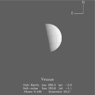
Figure 1:

Figure 2:

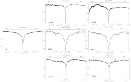
Figure 3:

Figure 4:

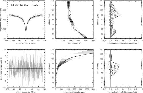
Figure 5:

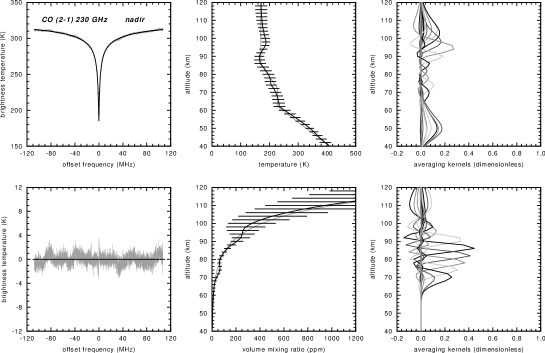
Figure 6:

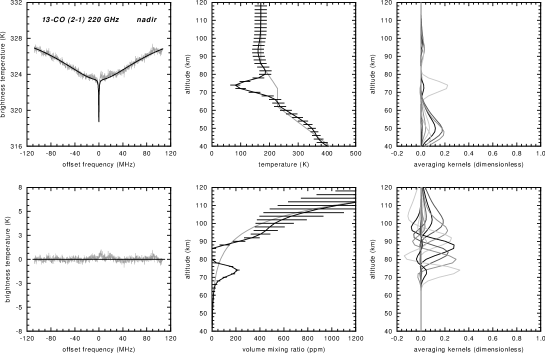
Figure 7:

Figure 8:

References

- Bertaux et al. (2007) Bertaux, J.-L., Vandaele, A., Korablev, O., Villard, et al, ., Nov. 2007. A warm layer in Venu’s cryosphere and high-altitude measurements of HF, HCl, H20 and HDO. Nature 450, 646–649.
- Clancy and Muhleman (1991) Clancy, R. T., Muhleman, D. O., Jan. 1991. Long-term (1979-1990) changes in the thermal, dynamical, and compositional structure of the Venus mesosphere as inferred from microwave spectral line observations of C-12O, C-13O, and CO-18. Icarus 89, 129–146.
- Clancy et al. (2003) Clancy, R. T., Sandor, B. J., Moriarty-Schieven, G. H., Jan. 2003. Observational definition of the Venus mesopause: vertical structure, diurnal variation, and temporal instability. Icarus 161, 1–16.
- Hartogh and Hartmann (1990) Hartogh, P., Hartmann, G. K., 1990. A high-resolution chirp transform spectrometer for microwave measurements. Meas. Sci. Technol. (1), 592–595.
- Hartogh and Jarchow (2004) Hartogh, P., Jarchow, C., 2004. The microwave brightness of planetary atmospheres, preparatory modeling for GREAT and HIFI. In: Amano, T., Kasai, Y., Manabe, T. (Eds.), Proceedings of the International Workshop on Critical Evaluation of mm-/submm-wave Spectroscopic Data for Atmospheric Observations, January 29-30, 2004, Ibaraki, Japan. Communications Research Laboratory, pp. 75–78.
- Jarchow (1998) Jarchow, C., Nov. 1998. Bestimmung atmosphärischer Wasserdampf- und Ozonprofile mittels bodengebundener Millimeterwellen-Fernerkundung. Ph.D. thesis, 1998.
- Jarchow and Hartogh (1995) Jarchow, C., Hartogh, P., 1995. Retrieval of data from ground-based microwave sensing of the middle atmosphere: Comparison of two inversion techniques. In: Global Process Monitoring and Remote Sensing of Ocean and Sea Ice, EUROPTO-Series 2586. SPIE, Bellingham, pp. 196–205.
- Kakar et al. (1976) Kakar, R. K., Waters, J. W., Wilson, W. J., Jan. 1976. Venus - Microwave detection of carbon monoxide. Science 191, 379–+.
- Lellouch et al. (1994) Lellouch, E., Goldstein, J. J., Rosenqvist, J., Bougher, S. W., Paubert, G., Aug. 1994. Global circulation, thermal structure, and carbon monoxide distribution in Venus’ mesosphere in 1991. Icarus 110, 315–339.
- Rodgers (1976) Rodgers, C. D., Nov. 1976. Retrieval of Atmospheric Temperature and Composition From Remote Measurements of Thermal Radiation. Reviews of Geophysics and Space Physics 14, 609–+.
- Schofield and Taylor (1983) Schofield, J. T., Taylor, F. W., Jan. 1983. Measurements of the mean, solar-fixed temperature and cloud structure of the middle atmosphere of Venus. Quarterly Journal of the Royal Meteorological Society 109, 57–80.
- Seiff and Kirk (1982) Seiff, A., Kirk, D. B., Jan. 1982. Structure of the Venus mesosphere and lower thermosphere from measurements during entry of the Pioneer Venus probes. Icarus 49, 49–70.
- Seiff et al. (1980) Seiff, A., Kirk, D. B., Young, R. E., Blanchard, R. C., Findlay, J. T., Kelly, G. M., Sommer, S. C., Dec. 1980. Measurements of thermal structure and thermal contrasts in the atmosphere of Venus and related dynamical observations. Journal of Geophysical Research 85, 7903–7933.
- Villanueva and Hartogh (2006) Villanueva, G., Hartogh, P., 2006. The high resolution chirp transform spectrometer for the SOFIA-GREAT instrument. Experimental Astronomy 18, 77–91.
- Wilson et al. (1981) Wilson, W. J., Klein, M. J., Kahar, R. K., Gulkis, S., Olsen, E. T., Ho, P. T. P., Mar. 1981. Venus. I - Carbon monoxide distribution and molecular-line searches. Icarus 45, 624–637.