On the exhaustive generation of convex permutominoes

Abstract

A permutomino of size $n$ is a polyomino determined by a pair $(\pi_{1},\pi_{2})$ of permutations of size $n+1$, such that $\pi_{1}(i)\neq\pi_{2}(i)$, for $1\leq i\leq n+1$. In this paper, after recalling some enumerative results about permutominoes, we give a first algorithm for the exhaustive generation of a particular class of permutominoes, the convex permutominoes, proving that its cost is proportional to the number of generated objects.

1 Introduction

A permutomino is a special polyomino, defined by two permutation matrices having the same size. The class of permutominoes was introduced by Incitti in [10] while studying the problem of determining the $\widetilde{R}$-polynomials (related to the Kazhdan-Lusztig R-polynomials) associated with a pair $(\mu,\nu)$ of permutations. In his paper Incitti gave a general definition of these combinatorial objects using some algebraic notions.

In this paper we use the definition of permutominoes given in [7] which does not use the algebraic notions and nevertheless, though different, it turns out to be equivalent to Incitti’s one.

The main results about permutominoes concern the enumeration of various subclasses of permutominoes and the characterization for the permutations defining these subclasses [3, 6, 7, 8, 9], while at our knowledge nothing exists about their generation. On the other hand, exhaustive generation of combinatorial objects [1, 4, 5] is an area of increasing interest. In fact, many practical questions in diverse areas, such as hardware and software testing, and combinatorial chemistry, require for their solution the exhaustive search through all objects in the class.

Actually, in [7] a recursive generation of all convex permutominoes of size $(n+1)$ from the ones of size $n$, according to the ECO method [2], is presented. Section 2 contains basic definitions and some enumerative results of convex permutominoes of size $n$. Section 3 recalls the recursive generation of convex permutominoes presented in [7] and Section 4 illustrates the exhaustive generating algorithm based on the recursive construction recalled in Section 3.

2 Basics on permutominoes

2.1 Definitions and properties

In order to define permutominoes we need to introduce polyominoes. In the plane $\mathbb{Z}\times\mathbb{Z}$ a cell is a unit square and a polyomino is a finite connected union of cells having no cut point. Polyominoes are defined up to translations. A column (row) of a polyomino is the intersection between the polyomino and an infinite strip of cells whose centers lie on a vertical (horizontal) line.

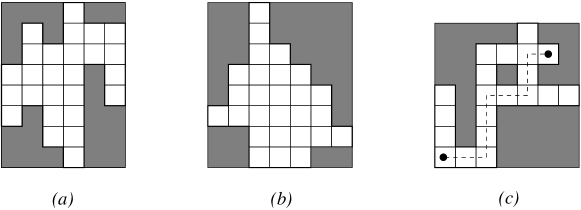
Figure 1: $(a)$ a column convex polyomino; $(b)$ a convex polyomino; $(c)$ a directed (not convex) polyomino with a hole.

In order to simplify many problems which are still open on the class of polyominoes, several subclasses were defined by combining two notions: the geometrical notion of convexity and the notion of directed growth. A polyomino is said to be column convex [row convex] if its intersection with any vertical [horizontal] line is convex (Figure 1 $(a)$). A polyomino is convex if it is both column and row convex (Figure 1 $(b)$). In a convex polyomino the semi-perimeter is given by the sum of the number of rows and columns, while the area is the number of its cells.

A polyomino $P$ is said to be directed when every cell of $P$ can be reached from a distinguished cell, called root (usually the bottom leftmost cell), by a path which is contained in $P$ and uses only north and east unit steps (Figure 1 $(c)$).

Let $P$ be a polyomino without holes having $n$ rows and $n$ columns, $n\geq 1$; without loss in generality, we assume that the bottom leftmost vertex of the polyomino minimal bounding rectangle lies in $(1,1)$. Let $A_{1},\ldots,A_{2(r+1)}$ be the sequence of the vertices of $P$ obtained by visiting the boundary in clockwise sense, starting from its leftmost point with minimal ordinate.

We say that $P$ is a permutomino if the sets ${{\cal P}_{1}}=\{A_{1},A_{3},\ldots,A_{2r+1}\}$ and ${{\cal P}_{2}}=\{A_{2},A_{4},\ldots,A_{2r+2}\}$ represent two permutations matrices of [$n+1$] = {1,2,…, $n+1$}. Obviously, if $P$ is a permutomino, then $r=n$, and $n$ is called the size of the permutomino. The two permutations defined by ${{\cal P}_{1}}$ and ${{\cal P}_{2}}$ are indicated by $(\,\pi_{1}(P),\,\pi_{2}(P)\,)$ (briefly, $(\pi_{1},\pi_{2})$), respectively (see Figure  2). Given a pair of permutations $\omega=(\mu,\,\nu)$ of $[n+1]$, we say that a permutomino $P$ is associated with $\omega$ if $\mu=\pi_{1}(P)$ and $\nu=\pi_{2}(P)$.

Figure 2: Two permutominoes and the associated permutations. The permutation $\pi_{1}$ (resp. $\pi_{2}$) is represented by black (resp. white) dots.

A permutomino is convex (directed) if it is a convex (directed) polyomino. A parallelogram permutomino is a directed and convex one having the $(1,1)$ and $(n,n)$ vertices in common with its minimal bounding square; a stack permutomino is a directed and convex one in which the bottom side of its minimal bounding square belongs to the permutomino itself.

The definition of permutominoes leads to the following remarkable property:

Proposition 1

Any permutomino $P$ has the property that, for each abscissa (ordinate) there exists exactly one vertical (horizontal) side in the boundary of $P$ having such coordinate. This property is also a sufficient condition for a polyomino to be a permutomino.

Starting from the leftmost point having minimal ordinate, and moving in a clockwise sense, the boundary of a permutomino $P$ can be encoded as a word in a four letter alphabet, $\{N,E,S,W\}$, where $N$ (resp., $E$, $S$, $W$) represents a north (resp. east, south, west) unit step. Any occurence of a sequence $NE$, $ES$, $SW$ or $WN$ in the word encoding $P$ defines a salient point of $P$, while any occurence of a sequence $EN$, $SE$, $WS$ or $NW$ defines a reentrant point of $P$ (see Figure 3). For simplicity of notation and to clarify the definition of the construction recalled in Section  3, the reentrant points of a convex permutomino are grouped in four classes; in practice, the reentrant point determined by a sequence EN (resp. SE, WS, NW) is represented with the symbol $\alpha$ (resp. $\beta$, $\gamma$, $\delta$).

Figure 3: The coding of the boundary of a permutomino, starting from A and moving in clockwise sense; its salient (resp. reentrant) points are indicated by black (resp. white) squares.

2.2 Previous enumerative results

Let us recall the main enumerative results concerning convex permutominoes. In [8, 9], using bijective techniques, the authors provide enumeration of various classes of convex permutominoes, including the parallelogram, the directed convex and the stack ones; moreover, a characterization of the permutations associated with permutominoes of each class is given. Let ${\cal C}_{n}$ (resp. ${\cal P}_{n}$, ${\cal D}_{n}$, ${\cal S}_{n}$) be the set of convex (resp. parallelogram, directed convex, stack) permutominoes of size $n$ and

$$\widetilde{\cal C}_{n}=\left\{\,\pi_{1}(P)\,:\,P\in{\cal C}_{n}\,\right\},\quad\widetilde{\cal P}_{n}=\left\{\,\pi_{1}(P)\,:\,P\in{\cal P}_{n}\,\right\},$$

$$\widetilde{\cal D}_{n}=\left\{\,\pi_{1}(P)\,:\,P\in{\cal D}_{n}\,\right\},\quad\widetilde{\cal S}_{n}=\left\{\,\pi_{1}(P)\,:\,P\in{\cal S}_{n}\,\right\}.$$

The enumeration results obtained in [8, 9] are shown in Table 1.

$Class\mbox{ }of\mbox{ }convex\mbox{ }$ $Number\mbox{ }of\mbox{ }convex$ $Associated\mbox{ }set$ $permutominoes$ $permutominoes\mbox{ }with\mbox{ }size\mbox{ }n$ $of\mbox{ }permutations$ $Parallelogram$ $|{\cal P}_{n}|=c_{n}$ $|\widetilde{\cal P}_{n}|=c_{n-1}$ $Directed\mbox{ }convex$ $|{\cal D}_{n}|=\frac{1}{2}b_{n}$ $|\widetilde{\cal D}_{n}|=b_{n-1}$ $Stack$ $|{\cal S}_{n}|=2^{n-1}$ $|\widetilde{\cal S}_{n}|=2^{n-1}$

Table 1: Enumeration results.

where $c_{n}$ is the $n$th Catalan number,

$$c_{n}=\frac{1}{n+1}{2n\choose n}$$

and $b_{n}$ are the central binomial coefficients

$$b_{n}={2n\choose n}.$$

In [7] it was proved, using the ECO method [2], that the number of convex permutominoes of size $n$ is:

$$2(n+3)4^{n-2}-\frac{n}{2}{2n\choose n},\quad n\geq 1.$$

The first terms of the sequence are

$1,4,18,84,394,1836,8468,\dots$

(sequence A126020 in [11]). The same enumerative result was obtained, using a different approach, by Boldi et al. [6].
An interesting study of combinatorial properties of the set $\widetilde{\cal C}_{n}$ is in [3].

3 ECO construction of convex permutominoes

In this section we recall the ECO construction of convex permutominoes as given in [7].

Let ${\cal C}_{n}$ be the set of convex permutominoes of size $n$ and let $P\in{\cal C}_{n}$; the number of cells in the rightmost column of $P$ is called the degree of $P$. Let us consider the following properties of a convex permutomino:

U1 : the uppermost cell of the rightmost column of $P$ has the maximal ordinate among all the cells of the permutomino;

U2 : the lowest cell of the rightmost column of $P$ has the minimal ordinate among all the cells of the permutomino.

According to the ECO method [2], it is necessary to define an operator $\vartheta:~{}{\cal C}_{n}~{}\rightarrow~{}2^{{\cal C}_{n+1}}$ which defines a recursive construction of all the convex permutominoes of size $(n+1)$ in a unique way from the objects of size $n$. The operator $\vartheta$ defined in [7] acts on a convex permutomino performing some local expansions on the cells of its rightmost column. Let $c_{1},\ldots,c_{n}$ (resp. $r_{1},\ldots,r_{n}$) be the columns (resp. rows) of a permutomino $P$ of size $n$ numbered from left to right (resp. bottom to top) and let $\ell(c_{i})$ (resp. $\ell(r_{i})$) be the number of cells in the $i$th column (resp. row), with $1\leq i\leq n$. The four operations of $\vartheta$, denoted by $(\alpha),(\beta),(\gamma)$ and ($\delta$) are defined as follows:

$(\alpha)$ if $P$ satisfies condition U1, then operation $(\alpha)$ adds a new column made of $\ell(c_{n})+1$ cells on the right of $c_{n}$, see Figure 4.

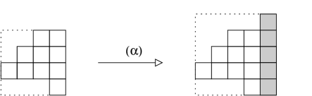
Figure 4: Operation $(\alpha)$; the added column has been highlighted

$(\beta)$ it can be performed on each cell of $c_{n}$; so let $d_{i}$ be the $i$th cell of $c_{n}$, from bottom to top, with $1\leq i\leq\ell(c_{n})$. Operation $(\beta)$ adds a new row above the row containing $d_{i}$ (of the same length), and add a new column on the right of $c_{n}$ made of $i$ cells, see Figure 5.

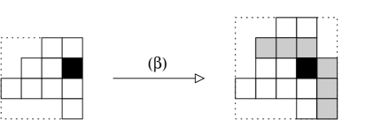
Figure 5: Operation $(\beta)$; the cell $d_{i}$ is filled in black , the added column and row have been highlighted

$(\gamma)$ it can be performed on each cell of $c_{n}$; so let $d_{i}$ be the $i$th cell of $c_{n}$, from bottom to top, with $1\leq i\leq\ell(c_{n})$. Operation $(\gamma)$ adds a new row below the row containing $d_{i}$ (of the same length), and add a new column on the right of $c_{n}$ made of $n-i+1$ cells, see Figure  6.

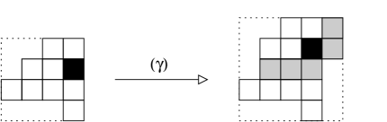
Figure 6: Operation $(\gamma)$; the cell $d_{i}$ is filled in black , the added column and row have been highlighted

$(\delta)$ if $P$ satisfies condition U2, then operation $(\delta)$ adds a new column made of $\ell(c_{n})+1$ cells on the right of $c_{n}$, see Figure  7.

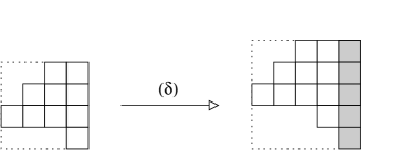
Figure 7: Operation $(\delta)$; the added column has been highlighted

Obviously in any case the obtained permutomino is a convex permutomino of size $n+1$.

We refer to [7] for further details and proofs.

4 The generating algorithm

Our aim is to illustrate an exhaustive generating algorithm for convex permutominoes, basing on the ECO construction recalled in previous section. In the sequel we will refer only to convex permutominoes, simply named “permutomino”.

First of all we define a subset of permutominoes of size $n$, the so called active permutominoes, then we will show the existence of a bijection between the active permutominoes of size $n$ and the set of permutominoes of size $n-1$. Finally, we will define the generating tree of permutominoes of size $n$.

4.1 Definition of active permutominoes

A permutomino $P$ is active if the following conditions hold:

1. the leftmost column contains only one cell, ($\ell(c_{1})=1$);

2. the leftmost reentrant point $\alpha$ has abscissa 2.

That is, the word encoding the boundary of an active permutomino begins with $"NEN\ldots$ and ends with $\ldots WW"$. In Figure 8 are depicted three active permutominoes of size 4, while in Figure 9 there are some permutominoes that, yet having only one cell in the leftmost column, are not active.

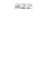
Figure 8: Three active permutominoes of size $4$

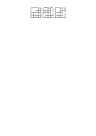
Figure 9: Some not active permutominoes of size $4$

Let $P$ be an active permutomino and let $\varrho$ be the row of $P$ containing the only cell in the leftmost column (in Figure 8 $\varrho$ is highlighted); $\varrho$ can be the bottom row but it is never the top row. From Proposition 1, $\varrho$ ends at the same abscissa of either the above and the below row, if it exists; so a configuration as that depicted in Figure 10 is not admissible. Therefore, if in an active permutomino $P$ of size $n$ we remove $\varrho$, we obtain a convex permutomino $P^{\prime}$ of size $(n-1)$.

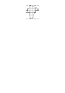
Figure 10: A not admissible configuration

Let $P^{\prime}$ be a permutomino of size $(n-1)$ and let $\varrho^{\prime}$ the row in $P^{\prime}$ containing the leftmost salient point with minimal ordinate (point A in Figure 3). If in $P^{\prime}$ we add, below $\varrho^{\prime}$, a row $\varrho$ one cell longer on the left and ending at the same abscissa of $\varrho^{\prime}$, we obtain an active permutomino $P$ of size $n$:

i. if $\varrho^{\prime}$ is the bottom row, the added row in $P^{\prime}$ is one cell longer on the left and therefore the new permutomino of size $n$ is convex and active (see Figure 11 a));

ii. if $\varrho^{\prime}=r_{i}$, with $1<i<n$, the row $r_{i-1}$ ends at the same abscissa of $\varrho^{\prime}$; so adding $\varrho$ we obtain a convex and active permutomino of size $n$ (see Figure  11 b)).

This means that it exists a bijection $\psi$ between the set ${\cal C}_{a,n}$ of active permutominoes and the set ${\cal C}_{n-1}$:

$$\psi\,:\,{\cal C}_{a,n}\,\to\,{\cal C}_{n-1}$$

such that $\psi(P)$ is the permutomino of size $n-1$ obtained by removing $\varrho$ from the active permutomino $P$ of size $n$.

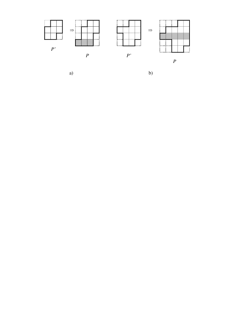
Figure 11: A permutomino $P^{\prime}$ of size $(n-1)$ and the corresponding permutomino $P$ of size $n$

4.2 The exhaustive generating algorithm

The algorithm we propose for the exhaustive generation of convex permutominoes of size $n$ is based on the bijection $\psi$, defined in Section 4.1, and on the ECO construction of permutominoes recalled in Section 3.

The generating process is described by an operator $\phi$ so defined:

$\phi$ Operator:

1. The first permutomino of the generating process is $P_{n}^{r}$, that is the permutomino of size $n$ associated with the pair of permutations $(\pi_{1},\pi_{2})$ of $[n+1]$:

   $$\pi_{1}=(1,2,3,\ldots,n,n+1)\qquad\pi_{2}=(2,3,4,\ldots,n+1,1)$$

   In Figure 12 is depicted $P_{n}^{r}$ of size 4.

2. $P_{n}^{r}$ is an active permutomino; let $\bar{P}^{r}$ the permutomino of size $(n-1)$ such that ${\bar{P}}^{r}=\psi(P_{n}^{r})$ ($\bar{P}^{r}$ is obtained by removing the bottom row of $P_{n}^{r}$ ).

3. Apply operations $(\beta)$, $(\gamma)$ and $(\delta)$ of ECO construction to $\bar{P}^{r}$. Every application generates a new convex permutomino of size $n$.

4. For each new active permutomino $Q$ repeat the following actions until active permutominoes are generated:

   4.1 remove the $\varrho$ row from $Q$ obtaining $\bar{Q}=\psi(Q)$;

   4.2 apply all the possible operations of the ECO construction to $\bar{Q}$. Every application generates a new convex permutomino of size $n$.

Figure 12: $P_{n}^{r}$ of size 4

Our strategy can be represented using a rooted tree, say ${\cal C}_{n}$-tree, so defined:

1. the root is $P_{n}^{r}$ and it is at level 0;

2. if $Q\in{\cal C}_{n}$-tree is an active permutomino at level $k\geq 0$, then $\phi(Q)=\vartheta(\psi(Q))$ ($\vartheta$ is the operator defined in the ECO construction) and every $P\in\phi(Q)$ is a son of $Q$ and it is at level $(k+1)$. For the sake of simplicity, we say that $P\in\phi^{k+1}(P_{n}^{r})$.

In Figure 13 ${\cal C}_{3}$-tree is illustrated.

Figure 13: ${\cal C}_{3}$-tree

Proposition 2

${\cal C}_{n}$-tree contains all and only the convex permutominoes of size $n$, i.e ${\cal C}_{n}$-tree $={\cal C}_{n}$.

Proof. [Only] The permutominoes in ${\cal C}_{n}$-tree are obtained from permutominoes of size $(n-1)$ by applying the ECO construction; so, as proved in [7], we generate permutominoes of size $n$. Therefore, since the permutominoes of size $(n-1)$ are each other different, the ones of size $n$ are different too.

[All] We must proof that for each permutomino $Q\in{\cal C}_{n}$ there exists a path from $P_{n}^{r}$ to $Q$, that is it exists a finite sequence $P_{0},P_{1},\ldots,P_{k}$ with $k\in\mathbb{N}$ and $P_{k}=Q$ such that:

• $P_{0}=P^{n}_{r}$;

• $P_{i+1}\in\phi(P_{i})$,      $0\leq$ i $\leq$ $k-1$.

Figure 14: ${\cal C}_{2}$-tree

In other words, we must prove that there exists $k\geq 1$ such that $Q\in\phi^{k}(P^{r}_{n})$. We know that the active permutominoes of size $n$ are as many as the permutominoes of size $(n-1)$. So it is sufficient to proof the following:

Proposition 3

All the active permutominoes of size $n$ are generated.

Proof. By induction on the size $n$.

Base. For $n=1$ there is only the permutomino containing one cell; if $n=2$ the unique active permutomino is $P^{r}_{2}$, (see Figure 14). So for $n\leq 2$ Proposition 3 yields.

Inductive hypothesis. Let us assume that all the permutominoes of size $(n-1)$ are generated and let ${\cal C}_{n-1}$-tree be the associated tree. Then, starting from the root $P_{n-1}^{r}$ it is possible to reach any permutomino of size $(n-1)$. So, for each permutomino $P_{n-1}\in{\cal C}_{n-1}$ there exists a $k$ such that:

$$P_{n-1}\in\phi^{k}(P_{n-1}^{r})$$

Inductive step. Let $\bar{P}_{n}$ be an active permutomino of size $n$ and let $Q_{n-1}=\psi(\bar{P}_{n})$ ($Q_{n-1}$ is obtained from $\bar{P}_{n}$ removing $\varrho$). So there exists $\bar{k}$ such that

$$Q_{n-1}\in\phi^{\bar{k}}(P_{n-1}^{r}).$$

But

$$P_{n-1}^{r}=\psi(P_{n}^{r})$$

so it follows that:

$$Q_{n-1}\in\phi^{\bar{k}}(P_{n}^{r})$$

that is, there is a path from the root $P_{n}^{r}$ to any permutomino of size $(n-1)$. Therefore, each permutomino of size $n$ is reachable from $P_{n}^{r}$.                 $\square$

4.3 Algorithm cost analysis

First of all, we will prove that the height of ${\cal C}_{n}$-tree is $n$. The proof is based on the following propositions.

Proposition 4

Using the ECO construction of Section 3, an active permutomino of size $n$ is generated by one and only one active permutomino of size $(n-1)$.

Proof. It follows straightforward from the ECO construction which never adds a column on the left containing one cell to the permutoninoes.          $\square$

Proposition 5

Given an active permutomino $Q$, the longest path starting from $Q$ has length $j$ if its $\alpha$ points lie in $(2,h),(3,h+1),\ldots,(j+1,h+j-1)$, $h$ being the ordinate of the lefmost $\alpha$ point.

Proof. The permutomino $\psi(Q)$ of size $(n-1)$ to which the ECO construction is applied, is obtained removing from $Q$ the row $\varrho$, so the leftmost $\alpha$ point of $Q$ is removed in $\psi(Q)$. Therefore, $\psi(Q)$ will be active, and then, from Proposition 4, it can generate new active permutominoes, only if it has an $\alpha$ point at abscissa 2; thus, $Q$ must have an $\alpha$ point at abscissa 3. In the same way, a permutomino generated from $\psi(Q)$ will be active only if $\psi(Q)$ has an $\alpha$ point at abscissa 3, that is if $Q$ has an $\alpha$ point at abscissa 4, and so on up to $(j+1)$.                                                                             $\square$

The permutomino $P_{n}^{r}$ has $(n-1)$ consecutive $\alpha$ points in $(2,2),\ldots,(n,n)$, so, from Proposition 5, the longest path starting from $P_{n}^{r}$ has length $(n-1)$. Therefore, the height of ${\cal C}_{n}$-tree is $n$.

From the generating alghorithm of Section 4.2 it follows that the generation of a permutomino $P$ at level $k$ in the ${\cal C}_{n}$-tree depends only on a permutomino at level $(k-1)$, that is, ${\cal C}_{n}$-tree is generated level by level. Therefore, since the generation of a permutomino of size $n$ from one of size $(n-1)$ has a constant cost, we may conclude that the cost of the exhaustive generating algorithm is proportional to the number of permutominoes of size $n$.

References

- [1] S. Bacchelli, E. Barcucci, E. Grazzini, E. Pergola, Exhaustive Generation Of Combinatorial Objects By ECO, Acta Informatica, 40 (8), 585–602 (2004).
- [2] E. Barcucci, A. Del Lungo, E. Pergola, R. Pinzani, ECO: a methodology for the Enumeration of Combinatorial Objects, J. Diff. Eq. and Appl., 5, 435–490 (1999).
- [3] A. Bernini, F. Di Santo, R. Pinzani, S. Rinaldi, Permutations defining convex permutominoes, J. of Integer Sequences, 10, Article 07.9.7 (2007).
- [4] A. Bernini, I. Fanti, E. Grazzini, An exhaustive generation algorithm for catalan objects and others, Pu.M.A., 17 (1-2), 39–53 (2006).
- [5] A. Bernini, E. Grazzini, E. Pergola, R. Pinzani, A general exhaustive generation algorithm for Gray structures, Acta Informatica, 44 (5), 361–376 (2007).
- [6] P. Boldi, V. Lonati, R. Radicioni, M. Santini, The number of convex permutominoes, Proc. of LATA 2007, International Conference on Language and Automata Theory and Applications, Tarragona, Spain, (2007).
- [7] F. Disanto, A. Frosini, R. Pinzani, S. Rinaldi, A closed formula for the number of convex permutominoes, The Electronic Journal of Combinatorics, 14, #R57, (2007).
- [8] I. Fanti, A. Frosini, E. Grazzini, R. Pinzani, S. Rinaldi, Polyominoes determined by permutations, Discrete Mathematics and Theoretical Computer Science AG, 381–390 (2006).
- [9] I. Fanti, A. Frosini, E. Grazzini, R. Pinzani and S. Rinaldi, Characterization and enumeration of some classes of permutominoes, (submitted)
- [10] F. Incitti, Permutation diagrams, fixed points and Kazdhan-Lusztig -polynomials, Ann. Comb., 10, N. 3, 369–387 (2006).
- [11] N.J.A. Sloane, On-Line Encyclopedia of Integer Sequences, http://www.research.att.com/~njas/sequences/.