Multi-setting Bell inequality for qudits

Abstract

We propose a generalized Bell inequality for two three-dimensional systems with three settings in each local measurement. It is shown that this inequality is maximally violated if local measurements are configured to be mutually unbiased and a composite state is maximally entangled. This feature is similar to Clauser-Horne-Shimony-Holt inequality for two qubits but is in contrast with the two types of inequalities, Collins-Gisin-Linden-Massar-Popescu and Son-Lee-Kim, for high-dimensional systems. The generalization to aribitrary prime-dimensional systems is discussed.

I Introduction

Nonlocality is a profound notion in quantum mechanics. Quantitative predictions by quantum mechanics are incompatible with constraints which local realism implies on a correlation of measurements between two separate systems. These constraints are called Bell inequalities Bell64 . A typical Bell inequality for bipartite two-dimensional systems (two qubits) was derived by Clauser, Horne, Shimony, and Holt (CHSH) CHSH69 , allowing more flexibility in local measurement configurations than the original Bell inequality Bell64 . Quantum mechanics maximally violates the CHSH inequality when the two qubits are in a maximally entangled state and each qubit is measured by two mutually unbiased bases C80 ; Horodecki . We observe that nonlocality for maximally entangled qubits is most strongly manifested by mutually unbiased bases, similarly to the complementarity principle.

Since the discovery by Bell Bell64 , investigation of nonlocality for more general systems has been regarded as one of the most important challenges in quantum mechanics and quantum information science Werner ; Garg80 ; GHZ89 ; Mermin90 ; ABK92 ; KGZ00 ; KKCZO02 ; CKKO02 ; CGLMP02 ; ACG04 ; Lee04 ; Cerf02 ; Cabello02 ; SLK06 ; Gisin92 . The studies include nonlocality without inequalities for three or more qubits, presented by Greenberger, Horne, and Zeilinger GHZ89 . In distinction with the bipartite qubit case, the contradiction between local realism and quantum mechanics can now be revealed by perfect correlations. Mermin immediately derived statistical inequalities for arbitrarily many qubits and showed that the degree of their violations exponentially increases with an increasing number of parties Mermin90 ; ABK92 . The nonlocality for multipartite systems plays an important role in quantum information processing, for instance, one way quantum computation with cluster states RB01 .

Generalization to higher dimensional systems (qudits) has also been investigated KGZ00 ; KKCZO02 ; CKKO02 ; CGLMP02 ; ACG04 ; Lee04 ; Cerf02 ; Cabello02 ; SLK06 . Nonlocality of two qudits was shown to be more robust against isotropic noises than that of two qubits by numerical analysis KGZ00 and by analytically deriving Collins-Gisin-Linden-Massar-Popescu (CGLMP) inequality CGLMP02 . Son et al. recently derived inequalities and showed their violations for arbitrary many qudits, including two qudits SLK06 . Such inequalities for two qudits can be applied to a bipartite division of many qubits, for instance, a division of $2n$ qubits into two parties, each having $n$ qubits, which is equivalent to a $2^{n}\times 2^{n}$ system. We may ask when such Bell inequalities for qudits are maximally violated: Are they maximally violated when a maximally entangled state and mutually unbiased measurements are employed, as in the CHSH inequality for two qubits? It was shown that the CGLMP inequality is maximally violated by a partially entangled state, not by any maximally entangled states, for two three-dimensional systems (qutrits) and further by mutually biased measurements ADGL02 . On the other hand, the inequality of Son et al. is maximally violated by a maximally entangled state, but still with mutually biased measurements. These features are “counter-intuitive” in the sense that there exists no nonlocality for neither entanglement nor unbiased measurements. They are also in contrast with the CHSH inequality which is maximally violated for a maximally entangled state and mutually unbiased measurements.

The generalized Bell inequalities mentioned above were derived by assuming that each observer is allowed to choose one of two possible settings in the local measurement. However, one may extend the number of measurement settings, as done for qubits in Ref. Z93 ; ZK97 ; NLP06 . We conjecture that the counter-intuitive features of the generalized Bell inequalities would be due to deficiency in the number of measurement settings, as $(d+1)$ mutually unbiased bases are possible for a prime or power-of-prime $d$-dimensional system.

In this paper, we propose a Bell inequality for two qutrits that is maximally violated when a maximally entangled state and mutually unbiased measurements are employed. For the purpose we allow each observer to choose one of three measurement settings. In addition generalization of our Bell inequality to prime-dimensional qudits is discussed.

II Three-setting Bell inequality for two qutrits

II.1 CHSH inequality for two qubits

Before presenting Bell inequality for two qutrits, we briefly discuss the CHSH inequality for two qubits CHSH69 as they have in common certain properties. Suppose two parties, Alice and Bob, are separated in a long distance and observe two qubits distributed to them. Alice and Bob each have two sets of measuring apparatus. They each choose independently one of the two sets in their possession and perform a measurement with that set. We call the two variables, whose values are determined by the measurements using Alice’s (Bob’s) two sets of apparatus, $A_{0}$ and $A_{1}$ ($B_{0}$ and $B_{1}$ ), respectively. We assign two possible values of $\pm 1$ to the outcome of the measurement on each variable. The CHSH inequality is a constraint on correlations between Alice’s and Bob’s measurement outcomes if local realistic description is assumed. The Bell function for CHSH inequality is given as BMR92 ,

$${\cal B}(\lambda)=A_{0}(\lambda)\left(B_{0}(\lambda)+B_{1}(\lambda)\right)+A_{1}(\lambda)\left(B_{0}(\lambda)-B_{1}(\lambda)\right),$$ (1)

where $\lambda$ is a collection of local hidden variables and the variables, $A_{i}(\lambda)$ and $B_{j}(\lambda)$, take $\pm 1$ depending on the hidden variables $\lambda$, respectively. According to the local hidden variable theory, the statistical average of the Bell function must satisfy the following inequality CHSH69 ; C80 ; BMR92 ,

$$-2\leq\langle{\cal B}\rangle\leq 2,$$ (2)

where the statistical average $\langle{\cal B}\rangle=\int d\lambda\rho(\lambda){\cal B}(\lambda)$ with a probability density distribution $\rho(\lambda)$.

Taking a quantum-mechanical description, the statistical average of the Bell function is replaced by a quantum average of the corresponding operator CHSH69 ; C80 ; BMR92 . The Bell operator, the counterpart to the classical Bell function of Eq. (1), is given as

$$\hat{\cal B}=\hat{A}_{0}\otimes\left(\hat{B}_{0}+\hat{B}_{1}\right)+\hat{A}_{1}\otimes\left(\hat{B}_{0}-\hat{B}_{1}\right),$$ (3)

where $\hat{A}_{i}$ and $\hat{B}_{j}$ are operators corresponding to the variables $A_{i}$ and $B_{j}$, respectively. As measurement outcomes are assumed to be $\pm 1$, each of the operators $\hat{A}_{i}$ and $\hat{B}_{j}$ has eigenvalues $\pm 1$.

A quantum expectation of the Bell operator $\hat{\cal B}$ can be shown to violate the CHSH inequality (2). Let the operators be

$$\hat{A}_{0}={\hat{\sigma}}_{x},\;\hat{A}_{1}={\hat{\sigma}}_{y},\;\hat{B}_{0}={\hat{\sigma}}_{x},\;\hat{B}_{1}={\hat{\sigma}}_{y},$$ (4)

where $\hat{\sigma}_{x,y}$ are Pauli operators. Further let the two qubits be in a maximally entangled state,

$$|\psi\rangle=\frac{1}{\sqrt{2}}\left(|00\rangle+(-1)^{1/4}|11\rangle\right),$$ (5)

where $\{|j\rangle\}\equiv\{|0\rangle,|1\rangle\}$ is a standard basis whose elements are eigenvectors of Pauli operator $\hat{\sigma}_{z}$. A straightforward algebraic calculation shows that the quantum expectation $\langle\psi|\hat{\cal B}|\psi\rangle$ is $2\sqrt{2}$ and violates the constraint of the CHSH inequality (2). This implies that any local hidden variable theories can not simulate the quantum-mechanical correlation.

For the two-qubit nonlocality, we would remark that a) each observer randomly chooses one of two possible settings in measuring his/her qubit, b) each measurement produces one of two possible outcomes $\pm 1$, and c) a quantum expectation can maximally violate the constraint, imposed by local realistic description, and reaches the quantum maximum $2\sqrt{2}$ if two conditions of a quantum state being maximally entangled and two local operators being mutually unbiased are satisfied C80 ; Horodecki .

II.2 Derivation of the three-setting Bell inequality for two qutrits

Now we derive a three-setting Bell inequality for two qutrits. Our derivation is motivated by the fact that Bell inequalities for high-dimensional systems, suggested in literatures, are maximally violated only when local operators are mutually biased and/or a quantum state is partially entangled, contrary to the CHSH inequality for two qubits BMR92 ; CGLMP02 ; ACG04 ; SLK06 . Alice and Bob now have three sets of measuring apparatus each, from which they each choose one and perform a measurement. The three variables whose values are determined by the measurements using Alice’s (Bob’s) three sets are referred to as $A_{0}$, $A_{1}$, and $A_{2}$ ($B_{0}$, $B_{1}$, and $B_{2}$), respectively. We assign three possible values of $1$, $\omega$, and $\omega^{2}$, where $\omega=\exp{(i2\pi/3)}$ is a primitive third root of unity, to the outcome of the measurement on each variable. As discussed for the CHSH inequality, the local realistic description implies that the values of the variables are predetermined by the local hidden variables $\lambda$: $A_{i}=A_{i}(\lambda)$ and $B_{j}=B_{j}(\lambda)$, and a statistical average of their correlations is given as

$$\langle A_{i}B_{j}\rangle=\int{d\lambda\rho(\lambda)}A_{i}(\lambda)B_{j}(\lambda),$$ (6)

where $\rho(\lambda)$ is the probability density distribution over $\lambda$: $\rho(\lambda)\geq 0$ and $\int{d\lambda\rho(\lambda)=1}$.

To derive a constraint for the classical correlations, consider the following Bell function,

$${\cal B}(\lambda)=\frac{1}{2}\sum_{n=1}^{2}{\sum_{i=0}^{2}{\sum_{j=0}^{2}{\omega^{nij}A_{i}^{n}(\lambda)B_{j}^{n}(\lambda)}}},$$ (7)

where $A_{i}^{n}$ ($B_{j}^{n}$) is the $n$-th power of $A_{i}$($B_{j}$). This Bell function has notable features: First, it contains higher-order correlations, while the CHSH inequality involves only the first-order correlations. In fact the second power of a dichotomic variable in the CHSH inequality is meaningless as it is just unity. On the other hand, the variables contained in Eq. (7) are trichotomic variables and thus their second powers have their own significance. Second, ${\cal B}(\lambda)$ has Bob’s (or Alice’s) variables in the form of Fourier transformation. In this perspective one may look at the CHSH inequality in the similar form and in this sense the Bell function in Eq. (7) generalizes CHSH to qutrits.

We find classical upper and lower bounds for the statistical average of the Bell function in Eq. (7). Note first that every statistical average of ${\cal B}(\lambda)$ satisfies,

$$\min_{\lambda}{\cal B}(\lambda)\leq\int{d\lambda\rho\left(\lambda\right)}{\cal B}(\lambda)\leq\max_{\lambda}{\cal B}(\lambda),$$ (8)

where $\min_{\lambda}{\cal B}(\lambda)$ ($\max_{\lambda}{\cal B}(\lambda)$) means a minimum (maximum) of ${\cal B}$ over $\lambda$. This is clear due to the fact that $\rho(\lambda)$ is a probability density distribution: $\rho(\lambda)\geq 0$ and $\int{d\lambda\rho(\lambda)=1}$. The classical upper and lower bounds are thus determined by finding the maximum and minimum of the Bell function ${\cal B}(\lambda)$ over $\lambda$. By definition, each variable takes an element in $\{1=\omega^{0},\omega,\omega^{2}\}$ so that $A_{i}(\lambda)=\omega^{a_{i}(\lambda)}$ and $B_{j}(\lambda)=\omega^{b_{j}(\lambda)}$ for some integer-valued functions $a_{i}(\lambda)$ and $b_{j}(\lambda)$ with respective to $\lambda$. Then Eq. (7) can be rewritten as

$${\cal B}(\lambda) = \frac{1}{2}\sum_{n=1}^{2}\sum_{i=0}^{2}\sum_{j=0}^{2}\left[{\omega^{n(a_{i}(\lambda)+b_{j}(\lambda)+Ij)}}\right]$$ (9)

$$= \frac{3}{2}\left(\sum_{i=0}^{2}\sum_{j=0}^{2}\delta(a_{i}(\lambda)+b_{j}(\lambda)+ij)-3\right),$$

where $\delta(a)=1$ if $a\equiv 0\bmod{3}$ and $\delta(a)=0$ otherwise. Here, we used the identity, $\sum_{n=0}^{2}{\omega^{an}}=3\delta(a)$. Determining the upper and lower bounds of the Bell function ${\cal B}(\lambda)$ reduces to finding the bounds of $\Delta={\sum_{i,j}{\delta({a_{i}+b_{j}+ij})}}$ over arbitrary integers $a_{i}$ and $b_{j}$ modulo 3.

Meanwhile, we present two useful facts resulting from a number theory (see Ref. AG76 ). First, for a given prime integer $d$, $Z_{d}=\left\{{0,1,...,d-1}\right\}$ is a complete set of residues modulo $d$ so that $aZ_{d}\equiv\{0a,1a,...,(d-1)a\}=Z_{d}$ for an arbitrary integer $a\neq 0$. For instance let $d=3$ and $a=2$. Then $aZ_{3}=\{0a,1a,2a\}=\{0,2,1\}=Z_{3}$. Second, for $a,b,c\in Z_{d}$, $ab\neq ac\bmod{d}$ if and only if $b\neq c\bmod{d}$.

Returning to the problem of finding the bounds of $\Delta$, consider a matrix with elements consisting of the arguments of the delta function in $\Delta$,

$$\begin{pmatrix}a_{0}+b_{0}&a_{0}+b_{1}&a_{0}+b_{2}\\ a_{1}+b_{0}&a_{1}+b_{1}+1&a_{1}+b_{2}+2\\ a_{2}+b_{0}&a_{2}+b_{1}+2&a_{2}+b_{2}+1\end{pmatrix}.$$ (10)

The maximum of $\Delta$, $\Delta_{\mathrm{max}}$, is decided by counting the number of matrix elements that can simultaneously be congruent to zero modulo 3. Suppose that two different elements in $i$-th row are both congruent to zero modulo $3$: For $j\neq k$,

$$a_{i}+b_{j}+ij=a_{i}+b_{k}+ik=0\mod{3}.$$ (11)

This is followed by

$$(b_{j}-b_{k})+i\left({j-k}\right)=0\mod{3}.$$ (12)

Then, the two elements in $l(\neq i)$-th row, $a_{l}+b_{j}+lj$ and $a_{l}+b_{k}+lk$ can not simultaneously be congruent to zero modulo 3. That is,

$$(a_{l}+b_{j}+lj)-(a_{l}+b_{k}+lk)=(b_{j}-b_{k})+l(j-k)\neq 0,$$ (13)

which results from Eq. (12) by noting $i\left({j-k}\right)\neq l\left({j-k}\right)\bmod{3}$ for $i\neq l\bmod{3}$. Similar conditions are also derived for columns. Under the conditions, consider a case in which all the elements at the first row are zero and then one element at the second or third row can be zero, resulting in $\Delta=5$. Consider another case in which the first two elements at the first row are zero and then one of the first two elements at the second or third row can be zero as well as the last element at the second or third row, resulting in $\Delta=6$. All other cases are equivalent to the two cases discussed. We thus obtain $\Delta_{\mathrm{max}}=6$, for instance, when $\{a_{0}=0,a_{1}=0,a_{2}=1,b_{0}=0,b_{1}=0,b_{2}=1\}$. The minimum of $\Delta$, $\Delta_{\mathrm{min}}=0$, is easily obtained by noting $\Delta\geq 0$ and $\Delta=0$ when $\{a_{0}=0,a_{1}=0,a_{2}=1,b_{0}=1,b_{1}=1,b_{2}=2\}$. The two bounds, $\Delta_{\mathrm{max}}$ and $\Delta_{\mathrm{min}}$ imply that the Bell function satisfies the following inequality,

$$-\frac{9}{2}\,\leq{\cal B}(\lambda)\,\leq\frac{9}{2}.$$ (14)

From both inequalities $(\ref{eq2})$ and $(\ref{eq9})$, therefore, every statistical average of ${\cal B}(\lambda)$ satisfies

$$-\frac{9}{2}\,\leq\langle{\cal B}\rangle\,\leq\frac{9}{2}.$$ (15)

II.3 Quantum violation of the three-setting Bell inequality for two qutrits

We now show that a quantum expectation violates the Bell inequality (15). The Bell operator corresponding to the classical Bell function in Eq. (7) is given as

$$\hat{\cal B}=\frac{1}{2}\sum_{n=1}^{2}{\sum_{i=0}^{2}{\sum_{j=0}^{2}{\omega^{nij}\hat{A}_{i}^{n}\otimes\hat{B}_{j}^{n}}}}.$$ (16)

Here, each operator $\hat{A}_{i}$ ($\hat{B}_{j}$) represents a measurement for $A_{i}$ ($B_{j}$) on Alice’s (Bob’s) qutrit. An orthogonal measurement of $M\in\{A_{i},B_{j}\}$ is described by a complete set of orthonormal basis vectors $\{|k\rangle_{M}\}$. Distinguishing the measurement outcomes is indicated by a set of eigenvalues. Let the set of eigenvalues be $\{1,\omega,\omega^{2}\}$, as the trichotomic variable $M$ takes an element in the set by definition. The measurement operator is then represented by $\hat{M}=\sum_{k=0}^{2}\omega^{k}|k\rangle_{MM}\langle k|$. In this representation each trichotomic operator $\hat{M}\in\{\hat{A}_{i},\hat{B}_{j}\}$ is unitary, satisfying ${\hat{M}}^{3}=\openone$ where $\openone$ is the identity operator Cerf02 ; Lee04 ; SLK06 . We note that the unitary operator $\hat{M}$ and its second power $\hat{M}^{2}$ have the same measurement basis just with different orderings of eigenvalues so that the introduction of higher powers does not alter the number of measurement settings in this work.

To see the quantum-mechanical violation, consider the following unitary operators,

$$\begin{matrix}\hat{A}_{0}=\hat{f}_{10},&\hat{A}_{1}=\omega^{2}\hat{f}_{11},&\hat{A}_{2}=\hat{f}_{12},\\ \hat{B}_{0}=\hat{f}_{10},&\hat{B}_{1}=\hat{f}_{12},&\hat{B}_{2}=\omega^{2}\hat{f}_{11},\end{matrix}$$ (17)

where $\{\hat{f}_{ij}\equiv\hat{X}^{i}\hat{Z}^{j}\}$ forms an orthogonal basis on the Hilbert-Schmidt space of operators such that $\mathrm{Tr}{\hat{f}_{ij}^{\dagger}\hat{f}_{kl}}=3\delta_{ik}\delta_{jl}$ and each $\hat{f}_{ij}$ is a trichotomic operator with eigenvalues $1$, $\omega$, and $\omega^{2}$. [It is known that every pair of operators in $\{\hat{f}_{01},\hat{f}_{10},\hat{f}_{11},\hat{f}_{12}\}$ is mutually unbiased Wootters ; BBRV02 .] The operators $\hat{X}$ and $\hat{Z}$ are $3$-dimensional Pauli operators G99 such that

$$\hat{X}|k\rangle=|k+1\rangle,\;\hat{Z}|k\rangle=\omega^{k}|k\rangle,\;\hat{X}^{3}=\openone,\hat{Z}^{3}=\openone,$$

where $\{|k\rangle\}$ is a standard orthonormal basis consisting of eigenstates of $\hat{Z}$. Consider further a maximally entangled state of qutrits,

$$\left|\psi\right\rangle=\openone\otimes\hat{P}|\psi_{0}\rangle,$$ (18)

where $|\psi_{0}\rangle=\sum_{k}|kk\rangle/\sqrt{3}$ and a phase shifter $\hat{P}=\sum_{k}\omega^{-k/3}|k\rangle\langle k|$.

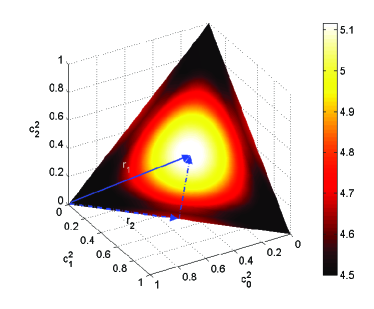
Figure 1: (color online) Maximum of the quantum Bell function for each quantum state in the form of Eq. (21), which we numerically obtain over all possible operators. Quantum states are denoted by points on the triangle, defined by the plane of $\sum_{i}c_{i}^{2}=1$ with $c_{i}^{2}$ being the Schmidt coefficients. The vertices represent products states of Schmidt rank 1, the points on the edges 2d entangled states of rank 2, and the interior points 3d entangled states of rank 3. It is evident that the quantum Bell function reaches its maximum over all possible quantum states if the state is 3d maximally entangled with $c_{0}^{2}=c_{1}^{2}=c_{2}^{2}=1/3$.

By using the unitary operators in Eq. (17) and the maximally entangled state in Eq. (18), the quantum expectation of the Bell operator $\hat{\cal B}$ is given as

$$\langle\psi|{\hat{\cal B}}|\psi\rangle = \langle\psi_{0}|\left(\openone\otimes\hat{P}^{\dagger}\right){\hat{\cal B}}\left(\openone\otimes\hat{P}\right)|\psi_{0}\rangle+\mathrm{c.c.}$$ (19)

$$= \langle\psi_{0}|\left(\frac{\sqrt{3}}{2}\,\omega^{1/12}\,\sum_{i=0}^{2}\hat{f}_{1i}\otimes\hat{f}_{1,-i}\right)|\psi_{0}\rangle+\mathrm{c.c.}$$

$$= 3\sqrt{3}\cos\left({\frac{\pi}{{18}}}\right)\approx 5.117,$$

where c.c. stands for the complex conjugate and the subscripts $i$ and $j$ in $\hat{f}_{ij}$ are congruent to positive residues modulo 3. In Eq. (19) we sequentially used two facts: a) The phase shifter $\hat{P}$ transforms Bob’s operators according to

$$\hat{P}^{\dagger}\hat{B}_{i}\hat{P} = \frac{\omega^{1/12}}{\sqrt{3}}\sum_{j=0}^{2}\omega^{(i-j+1)j}\hat{f}_{1j}.$$ (20)

b) The maximally entangled state $|\psi_{0}\rangle$ is a common eigenstate of three composite operators, that is, $\hat{f}_{1i}\otimes\hat{f}_{1,-i}|\psi_{0}\rangle=|\psi_{0}\rangle$ for all $i=0,1,2$, implying the perfect correlations for these composite variables. Then, the quantum expectation in Eq. (19), $3\sqrt{3}\cos(\pi/18)\approx 5.117$ clearly exceeds the classical upper bound $9/2=4.5$ of Bell inequality (15). This shows the nonlocality for two qutrits with three settings of local measurements by each observer.

Figure 2: Maximum of the quantum Bell function $B_{Q}$ with respect to the degree of entanglement $E$ for quantum states on the routes (a) $r_{1}$ and (b) $r_{2}$, shown in Fig. 1, from the product state $|00\rangle$ to the 3d maximally entangled state $(|00\rangle+|11\rangle+|22\rangle)/\sqrt{3}$. The route $r_{1}$ includes 3d entangled states, as in Eq. (21), with $c_{2}=c_{1}$ and $c_{1}\leq c_{0}$. The route $r_{2}$ includes 2d entangled states with $c_{2}=0$ and then 3d entangled states with $c_{0}=c_{1}$ and $c_{1}\geq c_{2}$. The global maximum is achieved for the 3d maximally entangled state in both cases.

II.4 Maximal violation of the three-setting Bell inequality

We investigate if the quantum expectation in Eq. (19) is maximal over all possible states. For the purpose it is necessary to optimize the quantum Bell function over all possible operators for each entangled state. By employing steepest decent method (see Ref. Son04 for the detailed methodology), we numerically find a set of such optimal unitary operators ($\hat{A}_{i}$ and $\hat{B}_{j}$) under local unitary transformations of SU(3). A pure state can in general be written, by Schmidt decomposition, as

$$|\psi^{\prime}\rangle=c_{0}|00\rangle+c_{1}|11\rangle+c_{2}|22\rangle,$$ (21)

where $c_{i}$ are non-negative real numbers, satisfying $\sum_{i}c_{i}^{2}=1$. In Fig. 1, composite states of two qutrits are denoted by points on the triangle, defined by the plane of $\sum_{i}c_{i}^{2}=1$ in the three dimensional vector space with the axes being Schmidt coefficients $c_{i}^{2}$. The vertices represent products states of Schmidt rank 1, the points on the edges two-dimensional (2d) entangled states of rank 2, and the interior points three-dimensional (3d) entangled states of rank 3. Fig. 1 presents the maximum of the quantum Bell function for a given quantum state $|\psi^{\prime}\rangle$, which we numerically obtain over all possible operators. It clearly shows that the quantum Bell function reaches its maximum value given in Eq. (19) over all possible quantum states if the state is 3d maximally entangled with $c_{0}^{2}=c_{1}^{2}=c_{2}^{2}=1/3$.

More explicitly, we consider quantum states on two routes $r_{1}$ and $r_{2}$, shown in Fig. 1, from the product state $|00\rangle$ to the 3d maximally entangled state $(|00\rangle+|11\rangle+|22\rangle)/\sqrt{3}$. These routes are chosen due to the three-fold rotational and reflectional symmetries of the quantum-state triangle under SU(3) transformations. Fig. 2 presents the maximum of the quantum Bell function $B_{Q}$ with respect to the degree of entanglement $E$ for quantum states on the routes (a) $r_{1}$ and (b) $r_{2}$, where $E=-\mbox{Tr}\hat{\rho}\log_{3}\hat{\rho}$ with $\hat{\rho}$ a marginal density operator. The route $r_{1}$ includes 3d entangled states, as in Eq. (21), with $c_{2}=c_{1}$ and $c_{0}\geq c_{1}$. It is clearly seen in Fig. 2(a) that, as the degree of entanglement $E$ is increased, $B_{Q}$ monotonically increases and reaches its maximum in Eq. (19) for the 3d maximally entangled state. The route $r_{2}$ includes 2d entangled states with $c_{2}=0$ and then 3d entangled states with $c_{0}=c_{1}$ and $c_{1}\geq c_{2}$. From Fig. 2(b), as increasing $E$, $B_{Q}$ increases to the local maximum when the quantum state is 2d maximally entangled, decreases slightly, and increases again to the global maximum in Eq. (19) when the state is 3d maximally entangled. Thus, it is evident that our quantum Bell function reaches its maximum in Eq. (19) only if a quantum state is 3d maximally entangled as in Eq. (18). It is worth noting that a partially entangled state results in the local maximum in our quantum Bell function, whereas CGLMP quantum Bell function admits the global maximum for a partially entangled state ADGL02 . In a sense our Bell inequality is free of the problem that the CGLMP Bell function has.

We remark that our Bell inequality is maximally violated by quantum mechanics if a composite state is maximally entangled and the local measurements are mutually unbiased as in Eqs. (17) and (18). Two measurements are said to be mutually unbiased if precise knowledge in one of them implies that all possible outcomes in the other are equally probable Lee03 ; Englert92 . Consider a nondegenerate and orthogonal measurement $M$ represented by a basis $\{|k\rangle_{M}\}$. Suppose a quantum system in $d$-dimensional Hilbert space is prepared in such a state that the outcome in the measurement $M$ can be predicted with certainty, for instance, the system’s state is $|i\rangle_{M}$. Let $N$ be another nondegenerate and orthogonal measurement represented by a basis $\{|j\rangle_{N}\}$. The measurement $N$ is mutually unbiased to $M$ if outcomes of measurement $N$ are equally probable for each $|i\rangle_{M}$:

$$p_{j|i}\equiv\left|{}_{N}\langle j|i\rangle_{M}\right|^{2}=\frac{1}{d},~{}~{}~{}~{}~{}~{}\forall j=1,2,..,d.$$ (22)

The two measurement bases, $\{|i\rangle_{M}\}$ and $\{|j\rangle_{N}\}$, are then said to be mutually unbiased. The eigenstates of $\hat{A}_{i}$ ($\hat{B}_{j}$) in Eq. (17) are easily determined by noting that the eigenstates $\{|k\rangle_{i}\}$ of $\hat{f}_{1i}$ are given as

$$|k\rangle_{i} = \frac{1}{\sqrt{3}}\sum_{l=0}^{2}\omega^{-il^{2}-kl}|l\rangle.$$ (23)

It was shown that two bases $\{|k\rangle_{i}\}$ and $\{|l\rangle_{j}\}$ are mutually unbiased if $i\neq j$ Wootters . The unitary operators $\hat{A}_{i}$ and $\hat{B}_{j}$ have the same bases as their corresponding $\hat{f}$’s in Eq. (17) with different orderings of eigenvalues so that arbitrary two local measurements represented by $\{\hat{A}_{i}\}$ or $\{\hat{B}_{j}\}$ are mutually unbiased.

We wish to remark here on the previous work by Buhrman and Massar BM05 , in which the authors introduced a Bell function and determined its quantum upper bound allowed for the general case of $d$-dimensional systems and $d$ measurement settings when local measurements on quantum entangled states are made. The quantum upper bound they determined is ”non-tight” in the sense that their Bell function cannot take on a value greater than that, but it has not been proven that this upper bound can actually be attained. Applying their result to our Bell operator of Eq.  (16), the quantum upper bound is $3\sqrt{3}\approx 5.196$. On the other hand, we have proven in Sec.  IID that $3\sqrt{3}\cos{\frac{\pi}{18}}\approx 5.117$ is the maximum value actually attainable, as given by Eq.  (19).

III Bell inequality for qudits

We generalize the Bell inequality for qutrits to $d$-dimensional systems, namely qudits, with $d$ a prime integer. A measurement on a qudit produces one of $d$ possible outcomes. For a generalized Bell inequality for qudits, two observers are allowed each to choose one of $d$ variables. Consider a classical Bell function for qudits,

$${\cal B}(\lambda)=\frac{1}{{d-1}}\sum_{n=1}^{d-1}{\sum_{i=0}^{d-1}{\sum_{j=0}^{d-1}{\omega^{nij}A_{i}^{n}(\lambda)B_{j}^{n}(\lambda)}}},$$ (24)

where $\omega$ is now a primitive $d$-th root of unity, i.e. $\omega=\exp(i2\pi/d)$, and $A_{i}(\lambda)=\omega^{a_{i}(\lambda)}$ and $B_{j}(\lambda)=\omega^{b_{j}(\lambda)}$ with $a_{i}(\lambda)$ and $b_{j}(\lambda)$ integer-valued functions of hidden variables $\lambda$. Eq. (24) is reduced to the CHSH Bell function in Eq. (1) if $d=2$ and to the two-qutrit function in Eq. (9) if $d=3$. Similarly to the two-qutrit case, the Bell function in Eq. (24) can be rewritten as,

$${\cal B}(\lambda)=\frac{d}{d-1}\left(\sum_{i=0}^{d-1}\sum_{j=0}^{d-1}\delta(a_{i}(\lambda)+b_{j}(\lambda)+ij)-d\right),$$ (25)

where $\delta(a)=1$ if $a=0\bmod{d}$ and $\delta(a)=0$ otherwise. As done in the two-qutrit case, we find classical upper and lower bounds by considering $\Delta=\sum_{i,j}\delta(a_{i}+b_{j}+ij)$. Using the similar arguments as given from Eq. (10) to (14), one obtains $\Delta_{\mathrm{max}}=3d-3$ and $\Delta_{\mathrm{min}}=0$. Then, the statistical average of the Bell function satisfies the following inequality,

$$-\frac{{d^{2}}}{{d-1}}\,\leq\langle{\cal B}\rangle\,\leq\frac{{d(2d-3)}}{{d-1}}$$ (26)

The quantum Bell operator, corresponding to the classical Bell function, is given as

$$\hat{\cal B}=\frac{1}{{d-1}}\sum_{n=1}^{d-1}{\sum_{i=0}^{d-1}{\sum_{j=0}^{d-1}{\omega^{nij}\hat{A}_{i}^{n}\otimes\hat{B}_{j}^{n}}}},$$ (27)

where $\hat{A}_{i}$ and $\hat{B}_{j}$ are local unitary operators with eigenvalues, $\{1,\omega,\omega^{2},...,\omega^{d-1}\}$. To show the nonlocality, let the local operators be

$$\hat{A}_{j}=\omega^{j(j+1)}\hat{f}_{1,j},\quad\hat{B}_{j}=\omega^{\left({\frac{{d+1}}{2}}\right)^{2}\left({j^{2}+2j}\right)}\hat{f}_{1,\frac{{\left({d+1}\right)^{2}}}{2}j}$$ (28)

where $\hat{f}_{i,j}=\hat{X}^{i}\hat{Z}^{j}$ and $\hat{X}$ and $\hat{Z}$ are now $d$-dimensional Pauli operators G99 . It is notable that $\hat{A}_{i}$ and $\hat{B}_{j}$ represent mutually unbiased measurements. Let further the two qudits be in a maximally entangled state,

$$|{\psi}\rangle=\openone\otimes\hat{P}\frac{1}{\sqrt{d}}\sum_{k=0}^{d-1}|kk\rangle.$$ (29)

where $\hat{P}=\sum_{k}\omega^{-\theta_{k}}|k\rangle\langle k|$. Here $\theta_{k}$ is defined by

$$\frac{\theta_{k}}{dk}=\left\{\begin{array}[]{ll}\frac{d-1}{8}+\frac{(d+1)^{2}}{4dk}\sum_{j=1}^{k}j^{2},&\mbox{for $d=8m+1$}\\ \frac{d+3}{8}-g_{d}+\frac{(d+1)^{2}}{4dk}\sum_{j=1}^{k}j^{2},&\mbox{for $d=8m+3$}\\ \frac{d+3}{8}+\frac{(d+1)^{2}}{4dk}\sum_{j=1}^{k}j^{2},&\mbox{for $d=8m+5$}\\ \frac{d-1}{8}-g_{d}+\frac{(d+1)^{2}}{4dk}\sum_{j=1}^{k}j^{2},&\mbox{for $d=8m+7$}\\ \end{array}\right.,$$ (34)

where $g_{d}=0$ for $d=8m+1$ or $8m+5$, and $g_{d}=1/4d$ for $d=8m+3$ or $8m+7$ for an integer $m$. From the mutually unbiased local measurements of Eq. (28) and the maximally entangled state in Eq. (29), the quantum expectation of the Bell operator is given as

$$\langle{\psi}|\hat{\cal B}|{\psi}\rangle=\frac{1}{d(d-1)}\sum_{n=1}^{d-1}\sum_{i,j,p=0}^{d-1}\omega^{\xi({i,j,p,n,g_{d}})},$$ (35)

where $\xi\left({i,j,p,n,g_{d}}\right)=-3ng_{d}+nij+\frac{{n(n-1)}}{2}i+inp+{\frac{3}{8}n(d-1)+\frac{3}{d}\left({\frac{{d+1}}{2}}\right)^{2}C(j,p,n)}$ and $C({j,p,n})=\sum_{k=1}^{n}{({j+p+k})^{2}}$. For $d=5$, the quantum expectation is $25(1+\sqrt{5})/8\approx 10.113$. This is clearly larger than the classical upper bound, $35/4=8.75$. For $d=17$, the quantum expectation $\langle\psi|\hat{\cal B}|\psi\rangle\approx 40.484$ exceeds 527/16=32.9375 of the classical upper bound, while no violations are found for $d=7,11,13$ if local unitary operators are employed as in Eq. (28).

Our Bell inequalities show relatively small degrees of violations. Ratios of quantum to classical maxima are given for $d=3,5,17$ as:

$$\frac{\langle\psi|\hat{\cal B}|\psi\rangle}{\langle{\cal B}\rangle}\approx\left\{\begin{array}[]{ll}1.137&~{}~{}~{}~{}~{}\mbox{for $d=3$}\\ 1.156&~{}~{}~{}~{}~{}\mbox{for $d=5$}\\ 1.229&~{}~{}~{}~{}~{}\mbox{for $d=17$}\end{array}\right..$$ (39)

These ratios are smaller than 1.414 and 1.436, those of CHSH inequality for qubits and CGLMP inequality for qutrits, respectively. However, it is interesting to observe that the ratios increase with respect to the dimension once the nonlocality appears.

Let us now examine the robustness of our Bell inequality against the white noise. For this purpose, we consider the state

$$\rho=p\left|\psi\right\rangle\left\langle\psi\right|+\frac{{\left({1-p}\right)}}{{d^{2}}}\openone\otimes\openone$$ (40)

This state represents a mixture of the pure state of Eq.  (29) and the fully mixed state, where $p$ is the relative weight of the pure state $\left|\psi\right\rangle$ with respect to the fully mixed state. We compute the lower bound $p_{min}$ of the $p$ value above which our Bell inequality is violated. Our calculation shows that $p_{min}=0.88,\;0.8653$ and $0.814$ for $d=3,\;5$ and $17$, respectively. One thus sees that our Bell inequality is more robust against the white noise as the dimension $d$ is increased, the tendency also observed in the CGLMP inequality.

IV Summary

We proposed a Bell inequality for two qutrits. This Bell inequality is maximally violated by quantum mechanics for mutually unbiased measurements and a maximally entangled state, whereas other Bell inequalities for high-dimensional systems such as CGLMP and that of Son et al. do not satisfy those conditions. This feature is consistent with the CHSH inequality of two qubits. Note that our Bell inequality consists of three settings of local measurements while CHSH, CGLMP and the inequality of Son et al. have two settings.

The Bell inequality for qutrits was generalized to prime-dimensional qudits. We investigated the generalized Bell inequalities for two qudits with the dimensions up to 17, finding the nonlocality for the dimensions $5$ and $17$. Further studies on the generalized Bell inequalities are encouraged to clarify if there are violations for higher dimensional systems and if the degree of nonlocality persistently increases with respect to the dimension once the nonlocality appears.

References

- (1) J. S. Bell, Physics 1, 195 (1964).
- (2) J. F. Clauser, M. A. Horne, A. Shimony, and R. A. Holt, Phys. Rev. Lett. 23, 880 (1969).
- (3) B. S. Cirel’son, Lett. Math. Phys. 4, 93 (1980).
- (4) R. Horodecki, P. Horodecki, and M. Horodecki, Phys. Lett. A 200, 340 (1995).
-
(5)
R. Werner, Open Problems,
http://www.imaph.tu-bs.de/qi/problems/1.html.
- (6) N. D. Mermin, Phys. Rev. D 22, 356 (1980); A. Garg and N. D. Mermin, Found. Phys. 14, 1 (1984).
- (7) D. M. Greenberger, M. A. Horne, and A. Zeilinger, in Bell’s Theorem, Quantum Theory and Conceptions of the Universe, edited by M. Kafatos (Kluwer Academic, Dordrecht, The Netherlands, 1989), pp. 69-72; D. M. Greenberger, M. A. Horne, A. Shimony, and A. Zeilinger, Am. J. Phys. 58, 1131 (1990).
- (8) N. D. Mermin, Phys. Rev. Lett. 65, 3373 (1990).
-
(9)
M. Ardehali, Phys. Rev. A 46, 5375 (1992) ;
A. V. Belinskii and D. N. Klyshko, Phys. Usp. 36, 653 (1993). - (10) D. Kaszlikowski, P Gnacinski, M. Zukowski, W. Miklaszewski and A. Zeilinger, Phys. Rev. Lett. 85, 4418 (2000).
- (11) D. Kaszlikowski, L. C. Kwek, J.-L. Chen, M. Zukowski, and C. H. Oh, Phys. Rev. A 65, 032118 (2002).
- (12) J. -L. Chen, D. Kaszlikowski, L. C. Kwek, and C. H. Oh, Mod. Phys. Lett. A 34, 2231 (2002).
- (13) D. Collins, N. Gisin, N. Linden, S. Massar, and S. Popescu, Phys. Rev. Lett. 88, 040404 (2002).
- (14) A. Acin, J. L. Chen, N. Gisin, D. Kaszlikowski, L.C. Kwek, C. H. Oh and M. Zukowski, Phys. Rev. Lett. 92, 250404 (2004).
- (15) J. Lee, S.-W. Lee, and M. S. Kim, Phys. Rev. A 73, 032316 (2006).
- (16) N. J. Cerf, S. Massar, and S. Pironio, Phys. Rev. Lett. 89, 080402 (2002).
- (17) A. Cabello, Phys. Rev. A 65, 062105 (2002).
- (18) W. Son, J. Lee, and M. S. Kim, Phys. Rev. Lett. 96, 060406 (2006); S.-W. Lee, Y. W. Cheong, and J. Lee, Phys. Rev. A 76, 032108 (2007).
- (19) N. Gisin and A. Peres, Phys. Lett. A 162, 15 (1992).
- (20) R. Raussendorf and H. J. Briegel, Phys. Rev. Lett. 86, 5188 (2001); O. Guhne, G. Toth, P. Hyllus, and H. J. Briegel, Phys. Rev. Lett. 95, 120405 (2005).
- (21) A. Acin, T. Durt, N. Gisin, and J. I. Latorre, Phys. Rev. A 65, 052325 (2002).
- (22) M. Zukowski, Phys. Lett. A 177, 290 (1993).
- (23) M. Zukowski and D. Kaszlikowski, Phys. Rev. A 56, R1682 (1997).
- (24) K. Nagata, W. Laskowski, and T. Paterek, Phys. Rev. A 74, 062109 (2006) and references therein.
- (25) S. L. Braunstein, A. Mann, and M. Revzen, Phys. Rev. Lett. 68, 3259 (1992).
- (26) W. W. Adams and L. J. Goldstein, Intoduction to Number Theory, Prentice-Hall, New Jersey, 1976.
- (27) W. K. Wootters and B. D. Fields, Ann. Phy. 191, 363 (1989); I. D. Ivanovic, J. Phys. A 14, 3241 (1981).
- (28) S. Bandyopadhyay, P. O. Boykin, V. Roychowdhury and F. Vatan, Algorithmica 34, 512 (2002).
- (29) D. Gottesman, Chaos, Solitons, and Fractals 10, 1749 (1999).
- (30) W. Son, J. Lee, and M. S. Kim, J. Phys. 37, 11897 (2004); J. Lim, J. Ryu, and J. Lee, in preparation.
- (31) B.-G. Englert, in Foundations of Quantum Mechanics, edited by T. D. Black, M. M. Nieto, H. S. Pilloff, M. O. Scully, and R. M. Sinclair, (World Scientific, Singapore, 1992); M. O. Scully, B.-G. Englert, and H. Walther, Nature 351, 111 (1991).
- (32) J. Lee, M. S. Kim, and Č. Brukner, Phys. Rev. Lett. 91, 087902 (2003).
- (33) H. Buhrman and S. Massar, Phys. Rev. A 72, 052103 (2005).