Self-sustained nonlinear waves in traffic flow

Abstract

In analogy to gas-dynamical detonation waves, which consist of a shock with an attached exothermic reaction zone, we consider herein nonlinear traveling wave solutions, termed “jamitons,” to the hyperbolic (“inviscid”) continuum traffic equations. Generic existence criteria are examined in the context of the Lax entropy conditions. Our analysis naturally precludes traveling wave solutions for which the shocks travel downstream more rapidly than individual vehicles. Consistent with recent experimental observations from a periodic roadway (Sugiyama et al. New Journal of Physics, 10, 2008), our numerical calculations show that, under appropriate road conditions, jamitons are attracting solutions, with the time evolution of the system converging towards a jamiton-dominated configuration. Jamitons are characterized by a sharp increase in density over a relatively compact section of the roadway. Applications of our analysis to traffic modeling and control are examined by way of a detailed example.

PACS: 89.40.Bb Land transportation; 47.10.ab Conservation laws; 47.40.Rs Detonation

1 Introduction and problem formulation

The economic costs in terms of lost productivity, atmospheric pollution and vehicular collisions associated with traffic jams are substantial both in developed and developing nations. As such, the discipline of traffic science has expanded significantly in recent decades, particularly from the point of view of theoretical modeling [1]. Borrowing terminology applied in Payne [2] and elsewhere, three generic categories describe the approaches considered in most previous analyses. “Microscopic” models, such as “follow the leader” studies [3] or “optimal velocity” studies [4] consider the individual (i.e. Lagrangian) response of a driver to his or her neighbors, in particular, the vehicle immediately ahead. “Mesoscopic” or “gas-kinetic macroscopic” analyses, such as the examinations of Phillips [5] and Helbing [6] take a statistical mechanics approach in which vehicle interactions are modeled using ideas familiar from kinetic theory. Finally “macroscopic” studies [2, 7, 8, 9, 10, 11, 12] model traffic flow using conservation laws and a suitable adaptation of the methods of continuum mechanics [13, 14], which yields governing equations similar to those from fluid mechanics. It is this latter category of analysis that is of interest here.

Treating the traffic flow as a continuum, we begin by considering a one dimensional Payne-Whitham model with periodic boundary conditions, i.e. vehicles on a circular track of length $0<\lambda<\infty\/$ [15]. The governing equations for mass and momentum are then (e.g. Kerner & Konhäuser [10])

$$\rho_{t}+(\rho\,u)_{x} = 0\/,$$ (1.1)

$$u_{t}+u\,u_{x}+\frac{1}{\rho}\,p_{x} = \frac{1}{\tau}\,\left(\tilde{u}-u\right)\/,$$ (1.2)

where the subscripts indicate differentiation, $\tau\/$ is a relaxation time-scale, $u\/$ is the traffic speed, and $\rho\/$ is the traffic density — with units of vehicles/length. The traffic pressure, $p\/$, which incorporates the effects of the “preventive” driving needed to compensate for the time delay $\tau\/$, is typically assumed to be an increasing function of the density only, i.e. $p=p(\rho)\/$ [11]. Here, in order to have a well-behaved theoretical formulation in the presence of shock waves [16], we shall assume that $p\/$ is a convex function of the specific volume $\mathrm{v}=1/\rho\/$ (road length per vehicle). This implies that $\mathrm{d}\/p/\mathrm{d}\/\mathrm{v}<0\/$ and $\mathrm{d}^{2}\/p/\mathrm{d}\/\mathrm{v}^{2}>0\/$, which holds for the functions typically assigned to $p\/$ in macroscopic models. Finally, $\tilde{u}=\tilde{u}(\rho)\/$ gives, for a particular traffic density, the desired or equilibrium speed to which the drivers try to adjust. The precise functional form of $\tilde{u}\/$ is, to a certain degree, rather arbitrary and indeed several variants have been proposed [1]. Generally, $\tilde{u}\/$ is a decreasing one-to-one function of the density, with $0<\tilde{u}(0)=\tilde{u}_{0}<\infty\/$ and $\tilde{u}(\rho_{M})=0\/$, where:

• $\rho_{M}\/$ denotes the maximum density, at which the vehicles are nearly “bumper-to-bumper” — thus $\ell=\rho_{M}^{-1}\/$ is the “effective” (uniform) vehicle length.

• $\tilde{u}_{0}\/$ is the drivers’ desired speed of travel on an otherwise empty road.

In this paper, we restrict ourselves to the representative form $\tilde{u}=\tilde{u}_{0}\,(1-\rho/\rho_{M})^{n}\/$, where $n\/$ is “close” to $1\/$. We defer the detailed treatment of the exact conditions on $\tilde{u}\/$ that guarantee the existence of self-sustained nonlinear traveling waves in traffic (termed “jamitons” herein) to a later publication.

Ubiquitous attributes of the solutions to continuum traffic models are stable shock-like features (see e.g. Kerner & Konhäuser [9] and Aw & Rascle [11]). In analyzing such structures, a dissipative term proportional to $u_{xx}\/$, analogous to the viscous term in the Navier-Stokes equations, is often added to the right-hand side of the momentum equation (1.2) in order to “smear out” discontinuities [1]. However, the physical rationale for this term is ambiguous and the proper functional form is therefore subject to debate. Solutions, such as those obtained by Kerner & Konhäuser [9], whose dynamics are non-trivially influenced by viscous dissipation must therefore be interpreted with care. Herein, an alternative line of inquiry is proposed: we seek self-sustained traveling wave solutions to the “inviscid” equations (1.1 – 1.2) on a periodic domain, where shocks are modeled by discontinuities, as in the standard theory of shocks for hyperbolic conservations laws [16]. As we demonstrate below, not only do such nonlinear traveling waves exist, but they have a structure similar to that of the self-sustained detonation waves in the Zel’dovich-von Neumann-Doering (ZND) theory [17]. According to the ZND description, detonation waves are modeled as shock waves with an attached exothermic reaction zone. In a self-sustained detonation wave, the flow downstream of the shock is subsonic relative to the shock, but accelerating to become sonic at some distance away from the shock. Hence, the flow behind a self-sustained detonation wave can be “transonic,” i.e. it may undergo a transition from subsonic to supersonic. The existence of the sonic point, the location where the flow speed relative to the shock equals the local sound speed, is the key feature in the ZND theory that allows one to solve for the speed and structure of the detonation wave. Its existence also means that the shock wave cannot be influenced by smooth disturbances from the flow further downstream so that the shock wave becomes self-sustained and independent of external driving mechanisms. Hence the sonic point is an “acoustic” information or event horizon [18].

For the nonlinear traffic waves to be discussed herein, this means that their formation, due to small initial perturbations, is analogous to the ignition and detonation that can occur in a meta-stable explosive medium. Although this analogy has not, to our knowledge, been reported in the traffic literature, the physical and mathematical similarities between detonation waves and hydraulic jumps, described by equations similar to (1.1) and (1.2), were recently pointed out by Kasimov [19]. (The analogy between hydraulic jumps and inert gas-dynamic shocks was recognized much earlier – see e.g. Gilmore et al. [20] and Stoker [21].) As with Kasimov’s analysis, our aim is to herein exploit such commonalities to gain additional understanding into the dynamics of traffic flows, in particular, the traffic jams that appear in the absence of bottlenecks and for no apparent reason. From this vantage point, novel insights are discerned over and above those that can be realized from the solution of a Riemann problem [11] or from the linear stability analysis of uniform base states (see e.g. Appendix C). Indeed, when such linear instabilities are present initially, our extensive numerical experiments suggest that the resulting “phantom jams” (see Helbing [1] and the many references therein) will ultimately saturate as jamitons. This observation provides a critical link between the initial and final states, the latter of which can, under select conditions (see e.g. § 5.3), be described analytically. Moreover, as we plan to illustrate in forthcoming publications, such self-sustained traffic shocks are also expected on non-periodic roads. Thus the model results presented below can be readily generalized beyond the mathematically convenient case of a closed circuit.

The rest of the paper is organized as follows: in § 2, we outline the basic requirements for (1.1) and (1.2) to exhibit traveling wave solutions. To demonstrate the generality of this analysis, we consider in § 3 modified forms for the momentum equation (developed by Aw & Rascle [11] and Helbing [12]). From this different starting point, the salient details of § 2 shall be reproduced. The analysis is further generalized in § 4, which considers a phase plane investigation of the governing equations from § 2 and § 3. A particular example is studied, both theoretically and numerically, in § 5 in which $\tilde{u}\/$ and $p\/$ are assigned particular functional forms. The impact of our findings on safe roadway design is briefly discussed. Conclusions are drawn in § 6.

2 Traveling wave solutions – jamitons

To determine periodic traveling wave solutions to the traffic flow equations (1.1) and (1.2), we begin by making the solution ansatz, $\rho=\rho\left(\eta\right)\/$ and $u=u\left(\eta\right)\/$, where the self-similar variable $\eta\/$ is defined by

$$\eta=\frac{x-s\/t}{\tau}\/.$$ (2.1)

Here $s\/$ is the speed, either positive or negative, of the traveling wave. Equation (1.1) then reduces to

$$\left\{\rho\left(u-s\right)\right\}_{\eta}=0,\quad\Longrightarrow\quad\rho=\frac{m}{u-s}\/,$$ (2.2)

where the constant $m\/$ denotes the mass flux of vehicles in the wave frame of reference. Substituting (2.2) into (1.2), we obtain

$$\frac{\mathrm{d}\/u}{\mathrm{d}\/\eta}=\frac{\left(u-s\right)\,\left(\tilde{u}-u\right)}{\left(u-s\right)^{2}-c^{2}}\/,$$ (2.3)

where we interpret $\tilde{u}=\tilde{u}(\rho)\/$ as a function of $u\/$ via (2.2). Here $c=(p_{\rho})^{1/2}>0\/$ is the “sound speed,” i.e. the speed at which infinitesimal perturbations move relative to the traffic flow.

Equation (2.3) is a first order ordinary differential equation and therefore, barring pathological and unphysical choices for $c\/$ and $\tilde{u}\/$, does not admit any smooth periodic solutions. Hence, the periodic traveling wave(s) — if they exist — must consist of monotone solutions to (2.3) that are connected by shocks. The simplest situation, as reproduced in the physical experiment of Sugiyama et al. [15], is one in which there is exactly one shock (with speed $s\/$) per period. The case of multiple shocks per period is more complex. We briefly address this situation in § 5.3.

Before going into the details of the solution, we recall that shocks must satisfy two sets of conditions to be admissible. First, they must satisfy the Rankine-Hugoniot conditions [11, 13, 14], which follow from the conservation of mass and momentum, and ensure that shocks do not become sources or sinks of mass and/or momentum. For the equations in (1.1 – 1.2), the Rankine-Hugoniot conditions take the form,

$$s\,[\rho] = [\rho u]\/$$ (i.e. conservation of mass), (2.4)

$$s\,[\rho u] = [p+\rho u^{2}]\/$$ (i.e. conservation of momentum), (2.5)

where $s\/$ is the shock speed and the brackets $[\;]\/$ indicate the jump in the enclosed variable across the shock discontinuity. These equations relate the upstream and downstream conditions at the shock. In particular, let the superscripts $+\/$ and $-\/$ denote the states immediately downstream (right) and upstream (left) of the shock, respectively. Then (2.4) is equivalent to

$$\rho^{+}\,(u^{+}-s)=m=\rho^{-}\,(u^{-}-s)\/,$$ (2.6)

where the constant $m\/$ is the mass flux across the shock. Of course, for a shock embedded within a jamiton, this $m\/$ is the same as the one in (2.2).

Second, shocks must satisfy the Lax “entropy” conditions [14, 16], which enforce dynamical stability. In the case of shocks in gas-dynamics, these conditions are equivalent to the statement that the entropy of a fluid parcel increases as it goes through the shock transition — hence the name. However, the existence of a physical entropy is not necessary for their formulation: stability considerations alone suffice. Furthermore, these conditions also guarantee that the shock evolution is causal.

For the particular system of equations in (1.1 – 1.2), the Lax entropy conditions — given below in (2.7 – 2.8) — state that one family of characteristics must converge into the shock path in space-time, while the other family must pass through it. Thus exactly two families of shocks are possible, as illustrated in figure 1: The left (respectively right) shocks have the left (respectively right) characteristics converging upon them.

Figure 1: Characteristics on both sides of a left (a) and right (b) shock in the frame of the shock. The flow direction is from left-to-right in (a) and right-to-left in (b). The equations of the characteristics are $C_{\pm}:\;\mathrm{d}\/\eta/\mathrm{d}\/t=(u-s\pm c)/\tau\/$, where $\eta\/$ is defined by (2.1), and $s\/$ is the shock speed.

In the context of the periodic traveling waves with a single shock per period, the above discussion implies that, in principle, two cases are possible: jamitons containing a left shock wherein the mass flux, $m\/$, is positive – see item 1. below, and jamitons containing a right shock wherein the mass flux, $m\/$, is negative – see item 2. below. However, as we argue after item 2., only jamitons with $m>0\/$ are mathematically consistent; self-sustained traveling waves carrying within them a right shock are not permitted. This is consistent with the experiment of Sugiyama et al. [15], as well as with one’s everyday driving experience: it is situations where individual vehicles overtake shocks (hence $m>0\/$) that are observed in reality, rather than the converse. Thus whereas in second order traffic models information in the form of shock waves can travel downstream faster than individual vehicles [22], the results in this paper show that this cannot happen in the form of a self-sustained traveling wave. Further to the analysis of Aw & Rascle [11] and Helbing [12], this observation lends additional support to the conclusion that second order models are not ipso facto flawed — see also Helbing [1], § III.D.7 and the references therein.

Let us now consider in some detail the two scenarios that can, in principle, arise for traveling waves with a single shock per period.

• The shock is the left shock, as in figure 1 a, so that

  $$\left(u-c\right)^{-}>s>\left(u-c\right)^{+}\/.$$ (2.7)

  In this case the mass flux must be positive, since $m=\rho^{-}\,\left(u^{-}-s\right)>\rho^{-}\,c^{-}>0\/$. Moreover, $\rho^{+}/\rho^{-}=\left(u-s\right)^{-}/\left(u-s\right)^{+}>c^{-}/c^{+}\/$, so that $\rho^{+}c^{+}>\rho^{-}c^{-}\/$. The traffic pressure $p\/$ is a convex function of $\mathrm{v}=\rho^{-1}\/$ (see § 1), hence $\rho\,c=(-\mathrm{d}\/p/\mathrm{d}\/\mathrm{v})^{1/2}\/$ is an increasing function of the traffic density. Thus $\rho^{+}\,c^{+}>\rho^{-}\,c^{-}$ implies that $\rho^{+}>\rho^{-}\/$. In other words, the shock is compressive: the traffic density increases as the vehicles pass through the shock, traveling from left to right. Conversely, since $u=s+m/\rho\/$, it follows that $u^{-}>u^{+}\/$ and, consequently, vehicles decelerate as they overtake the shock. It should then be clear that these shocks have all the familiar properties of traffic jams.

  We conclude that for a traveling wave with a left shock, the continuous solution of (2.1 – 2.3) must have a decreasing density, $\mathrm{d}\/\rho/\mathrm{d}\/\eta<0\/$, and an increasing velocity, $\mathrm{d}\/u/\mathrm{d}\/\eta>0\/$. This follows because the solution must be a monotone function of $\eta\/$, and must connect the post-shock state $\left(\rho^{+}\/,\,u^{+}\right)\/$ in one shock, to the pre-shock state $\left(\rho^{-}\/,\,u^{-}\right)\/$ in the subsequent shock across a period in $\eta\/$ — say from $\eta=0\/$ to $\eta=\lambda\/$.

• The shock is the right shock, as in figure 1 b, so that

  $$\left(u+c\right)^{-}>s>\left(u+c\right)^{+}\/.$$ (2.8)

  The mass flux now is negative, since $m=\rho^{+}\,\left(u-s\right)^{+}<-\rho^{+}\,c^{+}<0\/$. As in item 1., it is straightforward to show that $u^{-}>u^{+}\/$ and $\rho^{-}>\rho^{+}\/$. For a traveling wave with a right shock, the continuous and monotone solution of (2.1 – 2.3) must have both the density and velocity increasing with $\eta\/$ (i.e. $\mathrm{d}\/\rho/\mathrm{d}\/\eta>0\/$ and $\mathrm{d}\/u/\mathrm{d}\/\eta>0\/$), in order to connect $\left(\rho^{+}\/,\,u^{+}\right)\/$ to $\left(\rho^{-}\/,\,u^{-}\right)\/$ across a period in $\eta\/$. Notice that the shock is again compressive: the traffic density (in the vehicles’ frame of reference) increases as vehicles pass through the shock. However, in this latter case, the shock overtakes the vehicles from behind, which accelerate as they pass through the shock transition. This is a clearly counter-intuitive situation, not observed in real traffic [22].

Fortunately, as we demonstrate next, traveling wave solutions with $m<0\/$ are mathematically inconsistent, which obviates the need to consider them any further. First, (2.2) is employed to rewrite (2.3) in the form

$$\frac{\mathrm{d}\/u}{\mathrm{d}\/\eta}=m\,\rho\,G(\rho\/,\,s\/,\,m)\/,$$ (2.9)

where

$$G=\frac{\tilde{u}-u}{m^{2}-\rho^{2}\,c^{2}}\/,$$ (2.10)

$m^{2}-\rho^{2}\,c^{2}=\rho^{2}\,\left\{(u-s)^{2}-c^{2}\right\}\/$, and $u=s+m/\rho\/$. Because $\mathrm{d}u/\mathrm{d}\eta>0\/$, a smooth solution connecting $\left(\rho^{+}\/,\,u^{+}\right)\/$ to $\left(\rho^{-}\/,\,u^{-}\right)\/$ requires $G<0\/$. However, $m^{2}-\rho^{2}\,c^{2}=\rho\,(u-s+c)\,(m-\rho\,c)\/$ and $m-\rho\,c<0\/$, and it follows from (2.8) that $(m^{2}-\rho^{2}\,c^{2})^{+}>0>(m^{2}-\rho^{2}\,c^{2})^{-}\/$. Thus $G<0\/$ requires $(\tilde{u}-u)^{+}<0<(\tilde{u}-u)^{-}\/$, which is impossible since $\tilde{u}(\rho)-u=\tilde{u}(\rho)-s-m/\rho\/$ is a strictly decreasing function of $\rho\/$: $\tilde{u}(\rho)\/$ decreases with increasing $\rho$ by assumption and $m<0\/$.

The difficulties documented in the previous paragraph are avoided for traveling waves with $m>0$. In this case, we demand a solution of (2.9) with $\mathrm{d}\/u/\mathrm{d}\/\eta>0\/$ and $\mathrm{d}\/\rho/\mathrm{d}\/\eta<0\/$, connecting $\left(\rho^{+}\/,\,u^{+}\right)\/$ to $\left(\rho^{-}\/,\,u^{-}\right)\/$. This in turn requires $G>0\/$ for $\rho^{-}<\rho<\rho^{+}\/$. The assumptions on $p=p(\rho)\/$ imply that $m^{2}-\rho^{2}\,c^{2}\/$ is a strictly decreasing function of $\rho\/$ (item 1.). Since $m^{2}-\rho^{2}\,c^{2}=\rho\,(u-s-c)\,(m+\rho\,c)\/$ with $m+\rho\,c>0\/$, it follows from (2.7) that $(m^{2}-\rho^{2}\,c^{2})^{-}>0>(m^{2}-\rho^{2}\,c^{2})^{+}\/$. We conclude therefore that $m^{2}-\rho^{2}\,c^{2}\/$ has a unique, multiplicity one, zero at some $\rho_{s}$, with $\rho^{-}<\rho_{s}<\rho^{+}\/$. In order for (2.9) to have a smooth solution with the desired properties, the numerator $\tilde{u}-u=\tilde{u}(\rho)-s-m/\rho\/$ must be such that

$$\left.\begin{array}[]{rl}\mbox{(a)}&\tilde{u}-u\;\;\mbox{has a simple zero at}\;\;\rho=\rho_{s}\/;\\ \mbox{(b)}&\tilde{u}-u>0\;\;\;\mbox{for}\;\;\;\rho^{-}\leq\rho<\rho_{s}\/;\rule{0.0pt}{12.80373pt}\\ \mbox{(c)}&\tilde{u}-u<0\;\;\;\mbox{for}\;\;\;\rho_{s}\,<\rho\leq\rho^{+}\/.\rule{0.0pt}{12.80373pt}\end{array}\right\}$$ (2.11)

This then guarantees not only that the zero in the denominator of (2.9 – 2.10) is cancelled by a zero of the same order in the numerator, but that the resulting regularized ordinary differential equation yields $\mathrm{d}\/u/\mathrm{d}\/\eta>0\/$ everywhere, as needed. Indeed, $\rho_{s}$ is the traffic density at the sonic point, with corresponding flow speed $u_{s}=s+m/\rho_{s}\/$.

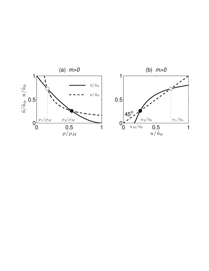
Figure 2: Panel (a) shows typical profiles for $\tilde{u}/\tilde{u}_{0}\/$ (solid curve) and $u/\tilde{u}_{0}\/$ (dashed curve) as functions of $\rho/\rho_{M}\/$, where $u=s+m/\rho\/$. Equivalently, these profiles may be plotted against $u/\tilde{u}_{0}\/$ by employing the transformation (2.2), as shown in panel (b) — the dashed curve is then just a line with unit slope. The two curves will either not intersect at all, be tangent at a single point, or have two transversal intersections. The case of interest to us is the one with two transversal intersections, as depicted here: $u_{2}\/$ is the intersection with a smaller velocity and a larger density $\rho_{2}=m/(u_{2}-s)\/$ — solid circles, while the other intersection (open circles) defines $u_{1}\/$ and $\rho_{1}\/$. It should be clear that, in order to satisfy the conditions in (2.11), the sonic point must coincide with $(u_{2}\/,\,\rho_{2})\/$. Finally, a physically meaningful solution requires $u>0\/$ everywhere. Hence, $u_{2}>0\/$ is needed. As shown by panel (b), this condition is equivalent to the statement: when $\tilde{u}=0\/$, that is $\rho=\rho_{M}\/$, the corresponding $u=u_{M}=s+m/\rho_{M}\/$ is positive.

Figure 2 illustrates the situation, with plots of $u\/$ and $\tilde{u}\/$ as functions of $\rho\/$ and $u\/$ for representative initial conditions $\rho^{+}\/$ and $u^{+}\/$. The shock speed, $s$, is here restricted by the inequalities $u^{+}>s>(u-c)^{+}\/$. Clearly, the conditions in (2.11) require that the sonic point values of the density, $\rho_{s}\/$, and velocity, $u_{s}\/$, coincide with $\rho_{2}\/$ and $u_{2}\/$. The sonic condition therefore reads

$$u_{2}=s+c\/(\rho_{2})\/,$$ (2.12)

from which the jamiton speed, $s\/$, can be determined. With $\rho_{2}\/$ and $u_{2}\/$ defined as functions of $(\rho^{+}\/,\,u^{+}\/,\,s)\/$ via figure 2, (2.12) is an algebraic equation that determines $s\/$ as a function of $(\rho^{+}\/,\,u^{+})\/$. In general, (2.12) must be solved numerically, however, in § 5 we provide an example where an analytic solution is possible. Finally, we point out that (i) the restriction $u_{M}>0\/$ must be imposed, where $u_{M}=s+m/\rho_{M}\/$ is the speed corresponding to the maximum traffic density, $\rho_{M}$; (ii) the cases of $u_{2}=u_{1}\/$, where $u_{1}$ is defined in figure 2, or of no intersections between the solid and dashed curves of figure 2 do not yield jamitons.

The methodology summarized above is reminiscent of the related analyses in gas dynamics [17, 18], shallow water theory [19, 23, 24], astrophysical accretion flow [25], and Newtonian flow in elastic tubes [26], where ordinary differential equations similar to (2.3) are obtained. Indeed, (2.12) is the exact analog of the Chapman-Jouguet condition in detonation theory [17].

Summarizing the above discussion, the following algorithm may be applied to determine the jamiton structure:

• For a prescribed downstream state, $(\rho^{+}\/,\,u^{+})\/$, the regularization condition (2.12) specifies the permissible value(s) for the wave speed, $s\/$.

• Once $s\/$ is determined, the state upstream of the shock, $(\rho^{-}\/,\,u^{-})$, is computed using the Rankine-Hugoniot conditions (2.4 – 2.5).

• Equation (2.3) is then integrated forward in $\eta\/$, from the initial condition $u=u^{+}\/$ up until $u=u^{-}\/$ is reached — the traffic density, $\rho\/$, follows automatically from (2.2). This defines the period $\lambda\/$ of the traveling wave or, equivalently, the circumference of the periodic roadway.

• The total number of vehicles, $\mathcal{N}\/$, which remains fixed in time when there are no on-ramps or off-ramps, is then evaluated from

  $$\mathcal{N}=\int_{0}^{\lambda}\rho\,\mathrm{d}\/x\/.$$ (2.13)

The jamitons thus obtained have the following properties: (i) The traffic speed smoothly increases in the downstream direction ($\mathrm{d}\/u/\mathrm{d}\/\eta>0\/$), except at the location of the shock, across which there is an abrupt drop in $u\/$; (ii) The traffic density smoothly decreases in the downstream direction ($\mathrm{d}\/\rho/\mathrm{d}\/\eta<0\/$), except at the location of the shock, across which there is an abrupt increase in $\rho\/$. This is consistent with the experimental observations of Sugiyama et al. [15].

The above algorithm provides a parameterization of the periodic jamitons using $(\rho^{+}\/,\,u^{+})\/$. Equivalent parameterizations, in terms of $(\rho^{-}\/,\,u^{-})\/$, are just as easy to produce. However, these are not necessarily ideal parameterizations. For example, in order to predict what jamiton configuration might arise from a given set of initial conditions, on a given closed roadway, a parameterization in terms of the roadway length, $\lambda\/$, and the total number of vehicles, $\mathcal{N}\/$, would be more desirable. On the other hand, for the example considered in § 5, and all the other case studies that we have examined to date, $\rho^{-}\/$ maps in a one-to-one fashion to $\mathcal{N}\/$. Thus, by applying the above algorithm, one can iteratively determine the unique traveling wave solution corresponding to particular choices for the functions $p\/$ and $\tilde{u}\/$, the parameters $\tau\/$ and $\lambda\/$, and the average traffic density $\rho_{avg}=\mathcal{N}\lambda^{-1}\/$.

3 Alternative description of the momentum equation

The existence of self-sustained shock solutions is not specific to the details of the continuum model used. It is, in fact, a feature of models involving hyperbolic conservation laws with forcing terms under rather generic conditions. To illustrate this point, we shall briefly consider the equations presented by Aw & Rascle [11] and Helbing [12]. These models were developed in response to the criticisms of Daganzo [22], who argued that second order models are necessarily flawed — they predict, for example, shocks overtaking individual vehicles in unsteady traffic flow, and negative vehicle speeds at the end of a stopped queue.

Aw & Rascle [11] overcome such limitations by applying a convective, rather than a spatial, derivative when modeling the effects of preventive driving (the anticipation term in their nomenclature). This leads to the momentum equation (1.2) being replaced by

$$(u+p)_{t}+u\,(u+p)_{x}=\frac{1}{\tau}\,\left(\tilde{u}-u\right)\/.$$ (3.1)

By substitution of the mass continuity equation (1.1), (3.1) can be re-written as

$$u_{t}+(u-c^{2}\,\rho)\,u_{x}=\frac{1}{\tau}\,\left(\tilde{u}-u\right)\/.$$ (3.2)

Introducing the self-similar variable $\eta\/$ defined by (2.1), it can be shown that

$$\frac{\mathrm{d}\/u}{\mathrm{d}\/\eta}=\frac{(u-s)\,(\tilde{u}-u)}{(u-s)^{2}-m\,c^{2}}\/,$$ (3.3)

which is identical to (2.3), except that the sonic point is now predicted to occur when $u-s=m^{1/2}c\/$. As before, the singularity of (3.3) — i.e. the sonic point, where the denominator vanishes — is regularized by aligning the sonic point with a root of $\tilde{u}-u\/$. The remainder of the analysis is entirely similar to that outlined previously for (1.1 – 1.2), with appropriate modifications to the shock conditions. Under the Aw & Rascle formulation, the Rankine-Hugoniot condition corresponding to the conservation of momentum takes the form

$$s\,[\rho\,(u+p)]=[\rho\,u\,p+\rho\,u^{2}]\/,$$ (3.4)

which replaces (2.5).

Helbing [12] generalized Aw & Rascle’s model one step further by defining two traffic pressures, both functions of $\rho\/$ and $u\/$, such that the momentum equation reads

$$u_{t}+u\,u_{x}+\frac{1}{\rho}\,\frac{\partial\/p_{1}}{\partial\/\rho}\,\rho_{x}+\frac{1}{\rho}\,\frac{\partial\/p_{2}}{\partial\/u}\,u_{x}=\frac{1}{\tau}\,(\tilde{u}-u)\/.$$ (3.5)

Proceeding as above, the following familiar expression can be readily obtained:

$$\frac{\mathrm{d}\/u}{\mathrm{d}\/\eta}=\frac{(u-s)\,(\tilde{u}-u)}{(u-s)^{2}-\varsigma^{2}}\/,$$ (3.6)

where

$$\varsigma^{2}=c_{1}^{2}+m\,c_{2}^{2}\,,$$ (3.7)

in which

$$c_{1}^{2}=\frac{\partial\/p_{1}}{\partial\/\rho}\quad\mbox{and}\quad c_{2}^{2}=-\frac{1}{\rho^{2}}\,\frac{\partial\/p_{2}}{\partial\/u}\/.$$

The Payne-Whitham and Aw & Rascle results may be recovered from (3.6) by setting, respectively, $p_{1}=p\/$, $p_{2}=0\/$; and $p_{1}=0\/$, $p_{2}=-u\,\rho^{2}\,\mathrm{d}\/p/\mathrm{d}\/\rho\/$.

4 Phase plane analysis

Generalizing the analyses of § 2 and § 3, $\mathrm{d}\/u/\mathrm{d}\/\eta\/$ may be expressed as

$$\frac{\mathrm{d}\/u}{\mathrm{d}\/\eta}=\frac{(u-s)\,(\tilde{u}-u)}{(u-s)^{2}-\Omega\,c^{2}}\/,$$ (4.1)

where $\Omega=1\/$ and $m\/$, respectively, for the Payne-Whitham and Aw & Rascle models. Further information regarding model behavior near the sonic point may be gleaned by introducing the phase plane variable $\xi\/$, and rewriting (4.1) as the following pair of ordinary differential equations

$$\frac{\mathrm{d}\/u}{\mathrm{d}\/\xi} = (u-s)\,(\tilde{u}-u)=F_{1}(u)\/,$$ (4.2)

$$\frac{\mathrm{d}\/\eta}{\mathrm{d}\/\xi} = (u-s)^{2}-\Omega\,c^{2}=F_{2}(u)\/.$$ (4.3)

Note that the sonic point is a critical point of (4.2) and (4.3). The Jacobian, $\mathcal{J}\/$, of the above pair of equations is then given by

$$\mathcal{J}=\left[\begin{array}[]{cc}F_{1,u}&0\\ F_{2,u}&0\end{array}\right]\/,$$ (4.4)

where

$$F_{1,u} = -(u-s)\left\{\frac{m\,\tilde{u}_{\rho}}{(u-s)^{2}}+1\right\}+\tilde{u}-u\/,$$ (4.5)

$$F_{2,u} = 2\,(u-s)+\frac{\Omega\,m}{(u-s)^{2}}\,p_{\rho\rho}\/,$$ (4.6)

in which

$$\tilde{u}_{\rho}\equiv\frac{\mathrm{d}\/\tilde{u}}{\mathrm{d}\/\rho}<0\quad\mbox{and}\quad p_{\rho\rho}\equiv\frac{\mathrm{d}^{2}\/p}{\mathrm{d}\/\rho^{2}}=\frac{\mathrm{d}\/c^{2}}{\mathrm{d}\/\rho}\/.$$

Therefore, at the sonic point the eigenvalues ($r_{1}\/$ and $r_{2}\/$) of $\mathcal{J}\/$ are given by

$$r_{1}=0\quad\mbox{and}\quad r_{2}=\frac{m\,|\tilde{u}_{\rho}|}{\Omega^{1/2}\,c}-\Omega^{1/2}\,c=F_{1,u}\/.$$ (4.7)

When $r_{2}>0\/$ (respectively $r_{2}<0\/$), $\,\mathrm{d}\/u/\mathrm{d}\/\eta>0\/$ (respectively $\mathrm{d}\/u/\mathrm{d}\/\eta<0\/$) at the sonic point. Because of the Lax entropy conditions described earlier, $u\/$ should be a monotonically increasing function of $\eta\/$ away from a shock, which in turn requires

$$r_{2}>0\quad\iff\quad m\,|\tilde{u}_{\rho}|>\Omega\,c^{2}\/.$$ (4.8)

Unfortunately, since $r_{1}=0\/$, the critical point is linearly degenerate. Thus a complete analysis of the solution behavior near this critical point requires a careful, but ultimately tangential, examination of the leading order contributions by nonlinearities. Nevertheless, an interesting observation can be made:

As we illustrate by way of example in § 5, $$r_{2}=0\/$$ coincides with the boundary wherein a constant uniform base state becomes unstable to infinitesimal disturbances — see figure 4 and Appendix C.    (4.9)

The theoretical underpinnings of this coincidence are not entirely clear. However, our numerical experiments show that there is a strong connection between jamitons and instabilities:

When a uniform traffic state is linearly unstable, the instability consistently saturates into a jamiton-dominated state.    (4.10)

For the more general analysis of Helbing [12] discussed at the end of § 3, $F_{2,u}\/$ is given by

$$F_{2,u} = 2\,(u-s)+\frac{m}{(u-s)^{2}}\,\varsigma^{2}_{\rho}\/,$$ (4.11)

$$= 2\,(u-s)+\frac{m}{(u-s)^{2}}\,p_{1,\rho\rho}+\frac{2(u-s)}{m}\,p_{2,u}-p_{2,u\rho}\/,$$

where $\varsigma^{2}\/$ is defined by (3.7). Given the form of the Jacobian matrix $\mathcal{J}\/$, modifying $F_{2,u}\/$ does not alter the eigenvalues $r_{1}\/$ and $r_{2}\/$.

5 An example

5.1 Preliminaries

To make the ideas of the previous sections more concrete, we consider herein particular forms for $p\/$ and $\tilde{u}\/$, and carefully examine the resulting range of solutions. As alluded to above, various expressions for $p\/$ and $\tilde{u}\/$ have been proposed in the traffic literature. Consistent with the spirit of previous studies (e.g. [9, 27]), our motivation is to select relatively simple functions so that the concepts of § 2 are succinctly illustrated with minimum algebraic investment. Thus, a Lighthill-Whitham-Richards forcing term of the form

$$\tilde{u}=\tilde{u}_{0}\,\left(1-\frac{\rho}{\rho_{M}}\right)\/,$$ (5.1)

is chosen. Moreover, by analogy with the shallow water equations [23], we select

$$p=\mbox{$\frac{1}{2}$}\,\beta\,\rho^{2}\/,$$ (5.2)

so that $p_{\rho}=c^{2}\propto\rho\;$ [11]. Alternatively, one could define $p\/$ to be singular in $\rho\/$, such that $p_{\rho}\propto\rho^{\varphi_{1}}/(\rho_{M}-\rho)^{\varphi_{2}}\/$ for some $\varphi_{1}\/,\,\varphi_{2}>0\/$. Whereas this, more complicated, choice for $p\/$ enforces $\rho_{M}\/$ as the maximum traffic density, the resulting algebraic relations become somewhat unwieldy. We therefore defer consideration of singular pressure functions to future studies.

Applying the above definitions to the Payne-Whitham model of § 1 yields

$$\frac{\mathrm{d}\/u}{\mathrm{d}\/\eta}=\frac{(u-s)\/\left\{\tilde{u}_{0}\/\left(1-\frac{m}{\rho_{M}\,(u-s)}\right)-u\right\}}{(u-s)^{2}-\frac{\beta\,m}{(u-s)}}\/.$$ (5.3)

The sonic point is then defined by

$$u-s=(\beta\,m)^{1/3}\/,$$ (5.4)

while the zeros of the numerator are given by

$$u=\{u_{1}\/,\,u_{2}\}=s+\mbox{$\frac{1}{2}$}\,(\tilde{u}_{0}-s)\pm\mbox{$\frac{1}{2}$}(\tilde{u}_{0}-s)\,\left\{1-\frac{4\,\tilde{u}_{0}\,m}{\rho_{M}\,(\tilde{u}_{0}-s)^{2}}\right\}^{1/2}\/.$$ (5.5)

The regularization condition (2.12) may then be written as

$$u_{2}=s+(\beta\,m)^{1/3}\/.$$ (5.6)

Equations (5.5) and (5.6) yield a cubic polynomial in $s\/$, with at most two physically-relevant roots. With $p\/$ defined by (5.2), the Rankine-Hugoniot conditions specified in (2.4) and (2.5) may be combined to yield

$$\frac{u^{-}-s}{u^{+}-s}=\frac{\rho^{+}}{\rho^{-}}=\mbox{$\frac{1}{2}$}\left\{-1+(1+8\,M_{-}^{2})^{1/2}\right\}\/,$$ (5.7)

where $M_{-}=|u^{-}-s|/(\beta\,\rho^{-})^{1/2}\,$ is the upstream Mach number [13, 14]. Finally, the non-trivial eigenvalue, $r_{2}\/$, of the Jacobian matrix given by (4.4), is, at the sonic point,

$$r_{2}=\frac{\tilde{u}_{0}}{\rho_{M}}\left(\frac{m^{2}}{\beta}\right)^{1/3}-\left(\beta\,m\right)^{1/3}\/.$$ (5.8)

Having regularized the ordinary differential equation given by (5.3) — i.e. upon defining $u_{2}\/$ by (5.6) and canceling $u-u_{2}\/$ from the numerator and denominator, the resultant differential equation has an exact, albeit implicit, solution given by

$$\eta = u^{+}-u+\frac{(\beta\,m)^{2/3}}{u_{1}-s}\,\mathrm{ln}\left(\frac{u-s}{u^{+}-s}\right)$$ (5.9)

$$+\left\{(\beta\,m)^{1/3}+u_{1}-s+\frac{(\beta\,m)^{2/3}}{u_{1}-s}\right\}\,\mathrm{ln}\left(\frac{u_{1}-u^{+}}{u_{1}-u}\right)\/.$$

A similar result is obtained in the study of roll waves in shallow water systems – see e.g. (4.18) in [23].

By definition, $u=u^{-}\/$ when $\eta=\lambda\/$, where $\lambda\/$ is the length of the periodic roadway. Therefore

$$\lambda = u^{+}-u^{-}+\frac{(\beta\,m)^{2/3}}{u_{1}-s}\,\mathrm{ln}\left(\frac{u^{-}-s}{u^{+}-s}\right)$$ (5.10)

$$+\left\{(\beta\,m)^{1/3}+u_{1}-s+\frac{(\beta\,m)^{2/3}}{u_{1}-s}\right\}\,\mathrm{ln}\left(\frac{u_{1}-u^{+}}{u_{1}-u^{-}}\right)\/.$$

Starting from (2.13), the total number of vehicles along the periodic circuit can be computed from

$$\mathcal{N}=\int_{0}^{\lambda}\rho\,\mathrm{d}\/x=\int_{0}^{\eta_{max}}\rho\,\mathrm{d}\/\eta=m\,\int_{u^{+}}^{u^{-}}\frac{1}{u-s}\,\left(\frac{\mathrm{d}\/u}{\mathrm{d}\/\eta}\right)^{-1}\mathrm{d}\/u\/.$$ (5.11)

Application of (5.3) in (5.11) yields then the explicit result

$$\mathcal{N} = m\,\tau\,\left\{\frac{(\beta\,m)^{2/3}}{u_{1}-s}\left\{\frac{u^{-}-u^{+}}{(u^{-}-s)\,(u^{+}-s)}\right\}+\right.$$ (5.12)

$$\frac{(\beta\,m)^{1/3}}{u_{1}-s}\left\{\frac{(\beta\,m)^{1/3}}{u_{1}-s}+1\right\}\,\mathrm{ln}\left\{\frac{(u^{-}-s)\,(u_{1}-u^{+})}{(u^{+}-s)\,(u_{1}-u^{-})}\right\}$$

$$+\left.\mathrm{ln}\left(\frac{u_{1}-u^{+}}{u_{1}-u^{-}}\right)\right\}\/.$$

Comparable exact solutions may also be determined when $p\propto\rho\;$, rather than $p\propto\rho^{2}\/$. These are presented in Appendix A.

5.2 Numerical method

In order to validate the aforementioned theoretical solutions and assess jamiton stability, we performed numerical simulations using a Lagrangian particle method [28]. In this method, each discrete particle, $i\/$, is assigned an initial position, $x_{i}\/$, and speed, $u_{i}\/$, which subsequently changes in time according to (5.13 – 5.18). The mass balance equation (1.1) is satisfied identically as the particles move, i.e. the numerical scheme is mass-conservative by construction. Importantly, the number of particles is typically two orders of magnitude larger than the number of vehicles. Thus, although a Lagrangian approach is employed, the numerical scheme constitutes a macroscopic, not a microscopic, description of traffic flow, albeit one with an intuitive link between the particle and vehicle density.

In general terms, the numerical method solves the differential equations

$$\begin{cases}\dot{x}_{i}&=u_{i}\/,\\ \dot{u}_{i}&=a_{i}\/,\end{cases}$$ (5.13)

where the particle acceleration, $\dot{u}_{i}\/$, is expressed as

$$\frac{\mathrm{d}\/u}{\mathrm{d}\/t}(x_{i}\/,\,t)=u_{t}(x_{i}\/,\,t)+u\,u_{x}(x_{i}\/,\,t)\/,$$ (5.14)

and

$$a_{i}=-\frac{c(\rho(x_{i}\/,\,t))^{2}}{\rho(x_{i}\/,\,t)}\,\rho_{x}(x_{i}\/,\,t)+\frac{1}{\tau}\,\left\{\tilde{u}(\rho(x_{i}\/,\,t))-u(x_{i}\/,\,t)\right\}\/.$$ (5.15)

The distance between adjacent particles $i\/$ and $i+1\/$ is defined by $d_{i+\frac{1}{2}}=x_{i+1}-x_{i}\/$. Then the inter-particle density is computed by

$$\rho_{i+\frac{1}{2}}=\frac{\vartheta}{d_{i+\frac{1}{2}}}\,,$$ (5.16)

where $\vartheta=\mathcal{N}/N_{p}\/$ — in which $\mathcal{N}\/$ is the number of vehicles (as specified by (2.13)) and $N_{p}\/$ is the number of particles. From (5.16), we define the vehicle density and the density gradient using a non-equidistant finite-difference stencil [29]:

$$\rho_{i}=\frac{d_{i+\frac{1}{2}}\,\rho_{i-\frac{1}{2}}+d_{i-\frac{1}{2}}\,\rho_{i+\frac{1}{2}}}{d_{i+\frac{1}{2}}+d_{i-\frac{1}{2}}}\/,$$ (5.17)

$$\rho_{i,x}=\frac{\rho_{i+\frac{1}{2}}-\rho_{i-\frac{1}{2}}}{\min\{d_{i+\frac{1}{2}}\/,\,2\,d_{i-\frac{1}{2}}\}+\min\{d_{i-\frac{1}{2}}\/,\,2\,d_{i+\frac{1}{2}}\}}\/.$$ (5.18)

The denominator in (5.18) is chosen so that, at the location of the shock, a given particle is influenced only by its nearest neighbor. The numerical scheme is stable — however, it produces bounded but unphysical oscillations wherever the vehicle density or speed changes abruptly. We suppress these features by adding a small amount of numerical viscosity, so that at each time step the velocity profile is smoothed out.

5.3 Results

Here we compare the theory of self-sustained traffic jams developed in § 2 and § 5.1, and numerical solutions of (1.1 – 1.2) — obtained using the algorithm of § 5.2. Employing the forcing and traffic pressure terms specified in (5.1) and (5.2), the equations have the non-dimensional form

$$\left.\begin{array}[]{rcl}\rho^{*}_{t^{*}}+(u^{*}\,\rho^{*})_{x^{*}}&=&0\/,\\ \Gamma_{1}\,\left(u^{*}_{t*}+u^{*}\,u^{*}_{x^{*}}\right)+(\Gamma_{2}/\rho^{*})\,p^{*}_{x^{*}}&=&1-\rho^{*}-u^{*}\/,\rule{0.0pt}{12.91663pt}\end{array}\right\}$$ (5.19)

where $\,\Gamma_{1}=\tau\,\tilde{u}_{0}\rho_{M}\/$, $\,\Gamma_{2}=\beta\,\tau\rho_{M}^{2}/\tilde{u}_{0}\/$, and $\,p^{*}=\frac{1}{2}(\rho^{*})^{2}\/$. The non-dimensional and dimensional variables are related via

$$\rho=\rho_{M}\,\rho^{*}\/,\quad u=\tilde{u}_{0}\,u^{*}\/,\quad x=\ell\,x^{*}\/,\quad\mbox{and}\quad t=(\ell/\tilde{u}_{0})\,t^{*}\/,$$ (5.20)

where $\ell=1/\rho_{M}\/$ is the effective vehicle length, defined earlier in § 1, the non-dimensional traveling wave speed is $s^{*}=s/\tilde{u}_{0}\/$, and the parameter $\tau$ is the adjustment time-scale required for an individual vehicle to effect an $\mathcal{O}(1)\/$ change in speed.

We consider as canonical modeling parameters $\ell=5\,$m, $\,\tilde{u}_{0}=30\,$m/s, $\,\tau=3.\bar{3}\,$s, and $\beta=450\,$m³/s${}^{2}\/$, whereby

$$\Gamma_{1}=20\quad\mbox{and}\quad\Gamma_{2}=2\/.$$ (5.21)

Note that $\beta=c^{2}/\rho$ is related to the speed at which disturbances propagate through traffic. Because a description, both theoretical and numerical, of jamitons is the central focus of the present analysis, we deliberately select a value for $\beta\/$ towards the lower end of its representative range, so as to facilitate an explicit display of jamiton properties and behavior. Hence, $\beta\/$, whose exact numerical value is likely difficult to estimate in any event, is chosen so that infinitesimal perturbations to a uniform base state develop into jamitons when the base-state density is 10% of $\rho_{M}\/$ — see Appendix C and, more particularly, the stability condition (5.22). Whereas larger numerical values for $\beta\/$ could be selected, corresponding to a more restrictive instability condition, the jamitons observed in these cases, though qualitatively equivalent to those described below, are somewhat less easy to visualize. The practical ramifications associated with choosing a larger value for $\beta\/$ are briefly addressed when we discuss (after examining the results in figure 4) the possibility of vehicular collisions.

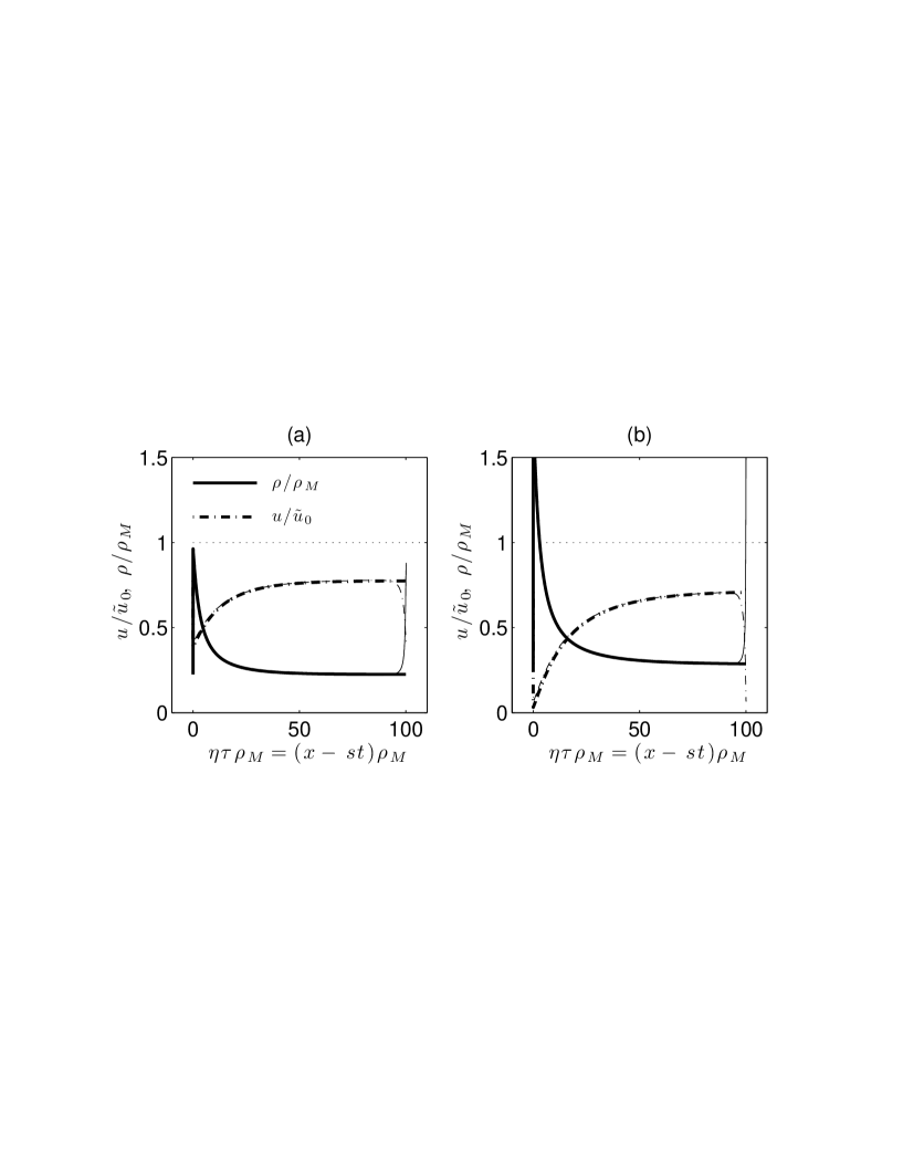
Figure 3: Comparison of theoretical (thick curves) and numerical (thin curves) solutions. The numerical solutions are the final, asymptotic state of an evolution started with a small perturbation of a uniform unstable base state — see (5.22). The agreement of this final state with the jamiton corresponding to the same road length, $\lambda\/$, and number of vehicles, $\mathcal{N}\/$, is remarkable. The plots show profiles of $\rho/\rho_{M}\/$ and $u/\tilde{u}_{0}\/$ versus $\eta\,\tau\,\rho_{M}=(x-st)\,\rho_{M}\/$. The equations and parameters are as in (5.19 – 5.21), with $\lambda=100\,\ell=500\,$m. In panel (a) $\,\mathcal{N}=27\/$ ($\rho_{avg}/\rho_{M}=0.272\/$). In panel (b) $\,\mathcal{N}=38\/$ ($\rho_{avg}/\rho_{M}=0.384\/$).

The steady-state variations of $u^{*}\/$ and $\rho^{*}\/$, as functions of the non-dimensional variable $\eta\,\tau\,\rho_{M}=x^{*}-s^{*}\,t^{*}\/$, are shown in figure 3 for a circular road of length $\lambda=100\,\ell\/$, with two different choices for the conserved number of vehicles, $\mathcal{N}\/$. The shock occurs at the two extreme ends of the horizontal domain, and connects the ratios $u^{-}/\tilde{u}_{0}\/$ to $u^{+}/\tilde{u}_{0}\/$, and $\rho^{-}/\rho_{M}\/$ to $\rho^{+}/\rho_{M}\/$. In figure 3 a, $\mathcal{N}=27\/$, and the maximum traffic density (i.e. $\rho^{+}\/$) is predicted to be just below $\rho_{M}\/$. Conversely, in figure 3 b, $\,\mathcal{N}\/$ is increased to $38\/$, which results in $\rho^{+}>\rho_{M}\/$. The physical implications of this result are considered in the following two paragraphs. Both theoretical and numerical data are included in figure 3. The comparison is very favorable, except right at the shock location — where the numerical scheme smears the shock.

Figure 4 indicates, as a function of the normalized average traffic density $\rho_{avg}/\rho_{M}\/$ (where $\rho_{avg}=\mathcal{N}/\lambda\/$), the range of possible solutions allowed by the model equations in § 5.1. The thick solid curves of figures 4 a,b show $\rho^{-}/\rho_{M}\/$ and $\rho^{+}/\rho_{M}\/$, respectively, whereas the thick dashed curves show $u^{-}/\tilde{u}_{0}\/$ and $u^{+}/\tilde{u}_{0}\/$, respectively. As with the discussion in § 2, we observe that, for a prescribed road length $\lambda\/$ and model parameters $\rho_{M}\/$, $\tilde{u}_{0}\/$, $\beta\/$, and $\tau\/$, the average density $\rho_{avg}\/$ (hence $\mathcal{N}\/$) uniquely determines the flow conditions to either side of the shock. Although the solid and dashed curves of figure 4 a do not proffer any particularly meaningful insights, those of figure 4 b are significant in that they predict the following forms of model breakdown: $\rho^{+}>\rho_{M}\/$ when $\rho_{avg}/\rho_{M}>0.277\/$ and $u^{+}<0\/$ when $\rho_{avg}/\rho_{M}>0.391\/$.

Rather than signifying a fundamental modeling flaw, observations of model breakdown provide helpful guidance in the safe design of modern roadways. In particular, for the choice of parameters germane to figure 4, vehicular collisions (i.e. $\rho\to\rho_{M}\/$) are anticipated once the average center-to-center separation between adjacent vehicles falls below approximately $3.6\,\ell\/$. Needless to say, this simple result is not universal for all types of traffic flow or roadway conditions. We consider herein a periodic track of prescribed length (500 m), particular functional forms for the traffic pressure, $p\/$, and equilibrium speed, $\tilde{u}\/$, and a liberal numerical value for $\beta\/$ such that jamitons appear even in relatively light traffic. In particular, choosing a larger value for $\beta\/$ would delay, though not necessarily avoid, the onset of vehicular collisions.

The roadway’s carrying capacity could, in principle, be increased if two or more traveling waves were to be forced rather than the single density spike considered here. However, our numerical simulations suggest that such bi- or multi-modal structures are often unstable, and that they quickly coalesce into a single structure. By contrast, unimodal traveling wave solutions of the type illustrated in figure 3 appear to be stable to small perturbations — except in the special case where the periodic roadway is made to be quite long, i.e. $\stackrel{{\scriptstyle>}}{{\sim}}2\,$km for the parameters appropriate to figures 3 and 4. On an extended circuit, the traveling wave solutions have a long, nearly constant state downstream of the shock — whose average density exceeds the requirement for linear stability discussed below. Thus infinitesimal perturbations may grow, leading to further traveling waves, albeit of slightly different amplitude from the original. Owing to the circuit length (i.e. $\stackrel{{\scriptstyle>}}{{\sim}}2\,$km, as compared to the $500\,$m long circuit considered in figure 3), these traveling waves are dynamically independent in that wave coalescence does not occur for a rather long time, if at all.

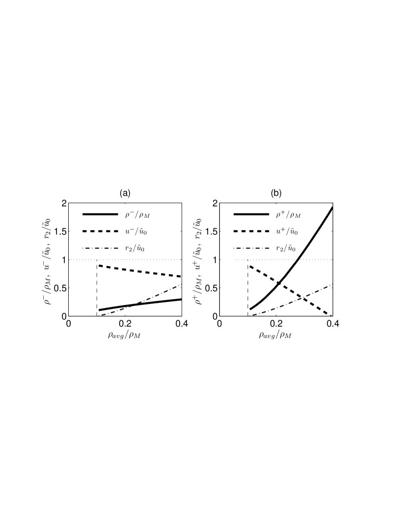
Figure 4: Parameters characterizing the exact jamiton solutions in § 5.1, for a fixed road length $\lambda=500$ m, as functions of the number of vehicles, $\mathcal{N}\/$. Specifically, curves of $\,\rho^{-}/\rho_{M}\/$, $\,\rho^{+}/\rho_{M}\/$, $\,u^{-}/\tilde{u}_{0}\/$, and $\,u^{+}/\tilde{u}_{0}\/$ versus $\rho_{avg}/\rho_{M}=\mathcal{N}/(\lambda\,\rho_{M})\/$ are shown, in addition to $\,r_{2}/\tilde{u}_{0}\/$ — as given in (5.8). The vertical dashed line is the stability boundary specified by (5.22). The equations and parameters are as in (5.19 – 5.21). Note that (i) $r_{2}\/$ goes through $0\/$ precisely at the stability boundary — see (4.9); (ii) the peak density $\rho^{+}\/$ reaches $\rho_{M}\/$ before $u^{+}\/$ becomes negative — see Appendix B.

While the above observations would benefit from the development of a more fundamental framework, it can be difficult to describe analytically the spatio-temporal stability of self-sustained traveling waves, due primarily to the transonic nature of the solution (see e.g. Stewart & Kasimov [18], Balmforth & Mandre [24] and Yu & Kevorkian [30]). Work is on-going to adapt nonlinear stability analyses for specific application to continuum traffic models.

In Appendix C we compute the boundary between linearly stable and unstable uniform base states, which is given by

$$\frac{\rho}{\rho_{M}}=\frac{\beta\,\rho_{M}}{\tilde{u}_{0}^{2}}\/.$$ (5.22)

In connection with this boundary, we point out the following facts, which together with (4.9 – 4.10), reinforce the point that there is a strong connection between jamitons and uniform flow instabilities.

• Figure 4 shows that $[\rho\,]\to 0\/$ and $[u]\to 0\/$, as $\rho_{avg}/\rho_{M}\downarrow\beta\,\rho_{M}/\tilde{u}_{0}^{2}\/$. Thus the jamiton amplitude becomes smaller as the corresponding uniform flow becomes less unstable, and vanishes altogether in the limit.

• The stability criterion (5.22) also specifies the location at which $u_{1}=u_{2}\/$, where $u_{1}\/$ and $u_{2}\/$ are defined in figure 2. Once $u_{1}\/$ and $u_{2}\/$ coalesce, no self-sustained shock wave may occur — since condition (a) in (2.11) fails. This is consistent with the discussion of the previous bullet, of course.

Thus jamitons become possible when the corresponding uniform state becomes unstable and — see (4.10) — the basic flow state changes from uniform flow to a jamiton-dominated state. In other words, evidence indicates that

A crucial bifurcation in the traffic flow behavior occurs at the stability boundary prescribed by (5.22). (5.23)

We defer a more in-depth investigation of this question for future work.

Finally, note that although the boundary specified by (5.22) is mathematically robust, in practice it may become “fuzzy” owing to the possible breakdowns of the continuum hypothesis, especially at low vehicle concentrations.

6 Conclusions

In this work, we have found and successfully exploited a strong similarity between gas-dynamical detonation waves and shocks in traffic flow, in order to develop a theory of “jamitons,” steady self-sustained traffic shocks. Jamitons naturally arise from small instabilities in relatively dense traffic flow, and can be interpreted as saturated phantom jams. While a single jamiton may not necessarily significantly delay individual vehicles, a succession of jamitons, as might arise during rush hour, for example, is expected to frustrate motorists over long lengths of roadway. Moreover, jamitons represent regions in which the traffic density increases dramatically over a relatively short distance [15] and, as such, are hot spots for vehicular collisions.

The analogy drawn above goes beyond the weaker analogy with inert shock waves in gas dynamics considered by Kerner, Klenov & Konhäuser [27]. Unlike inert shocks, detonation waves can be self-sustained, due to the existence of a sonic point in direct correspondence with the traffic model we consider here.

Using the Lax entropy conditions for hyperbolic conservation laws, we show that for realistic pressure and equilibrium-speed functions, the only allowable self-sustained shocks are those that are overtaken by individual vehicles. Moreover, for the simple, but widely-applied, choices $\tilde{u}=\tilde{u}_{0}(1-\rho/\rho_{M})\/$ and $p\propto\rho^{\gamma}\/$, with $\gamma=1\/,\,2\/$, we are able to describe the jamiton structure analytically. Theoretical solutions show excellent agreement with the output from direct numerical simulations of the governing system.

Examples of jamitons with $\gamma=2\/$ are illustrated in figure 3. Beyond a critical average density, we predict solutions for which the density immediately downstream of the shock exceeds the maximum allowable density, $\rho_{M}\/$, corresponding, physically, to a state of vehicular collisions (figure 4). Such instances offer important design insights for roadways; most obviously, it is advantageous to choose speed limits and roadway carrying capacities so as to avoid circumstances where densities with $\rho\stackrel{{\scriptstyle>}}{{\sim}}\rho_{M}\/$ are “triggered” (say, by a jamiton) anywhere within the domain.

Having identified self-sustained traveling wave solutions in traffic flow, a major objective of future research is to ascertain their spatio-temporal stability. Some of the analytical challenges associated with this line of inquiry are identified in § 5.3. Resolving issues of stability offers the possibility of increasing roadway efficiency, for example, by exciting multiple traveling waves of relatively low density as compared to the single density spike exhibited in figure 3. We hope to report on the results of such an analysis soon.

Acknowledgments
Partial support for J.-C. Nave, R. R. Rosales and B. Seibold was provided through NSF grant DMS-0813648. Funding for A. R. Kasimov was provided through the AFOSR Young Investigator Program grant FA9550-08-1-0035 (Program Manager Dr. Fariba Fahroo). We thank Dr. P.M. Reis for bringing to our attention the study of Sugiyama et al. [15].

Appendix A Exact solutions when $p\propto\rho\/$

Equations (5.9), (5.10) and (5.12) specify, respectively, exact analytical solutions for $u\/$, $\lambda\/$ and $\mathcal{N}\/$ when $p\propto\rho^{2}\/$. Corresponding expressions, valid when $p\propto\rho\/$, are given by

$$\eta=u^{+}-u+\left(u_{1}-s+\beta^{1/2}\right)\,\mathrm{ln}\left(\frac{u_{1}-u^{+}}{u_{1}-u}\right)\/,$$ (A.1)

$$\lambda=u^{+}-u^{-}+\left(u_{1}-s+\beta^{1/2}\right)\,\mathrm{ln}\left(\frac{u_{1}-u^{+}}{u_{1}-u^{-}}\right)\/,$$ (A.2)

and

$$\mathcal{N}=m\,\tau\,\left\{\frac{\beta}{u_{1}-s}\,\mathrm{ln}\left(\frac{u^{-}-s}{u^{+}-s}\right)+\left(1+\frac{\beta}{u_{1}-s}\right)\,\mathrm{ln}\left(\frac{u_{1}-u^{+}}{u_{1}-u^{-}}\right)\right\}\/,$$ (A.3)

respectively. As before, the traffic speed is given as an implicit function of $\eta\/$ in (A.1).

Appendix B Model behavior for $\rho>\rho_{M}\/$

From the discussion of § 5, vehicular collisions are forecast once $\rho^{+}=\rho_{M}\/$, whereas nonsensical vehicle speeds are predicted once $u^{+}<0\/$. It is demonstrated herein that the former condition is necessarily achieved before the latter.

Equation (2.2) shows that

$$\rho^{+}\,(u^{+}-s)=\rho_{M}\,(u_{M}-s)=m>0\/,$$ (B.1)

where $u_{M}\/$, which must be positive for jamitons to exist, is defined in figure 2 b. As $u^{+}\to 0\/$, the left-hand side of (B.1) approaches $-\rho^{+}\,s\/$, demonstrating that $s<0\/$. In this limit, therefore,

$$\frac{\rho^{+}}{\rho_{M}}=\frac{u_{M}-s}{|s|}>1\/.$$ (B.2)

This result can be understood intuitively by examining the functional form of the Lighthill-Whitham-Richards forcing term (see (5.1)): $\tilde{u}<0\/$ requires $\rho>\rho_{M}\/$. Clearly, the sensible alternative is to define $\tilde{u}=0\/$ for $\rho>\rho_{M}\/$. The point is moot, however: this amounts to correcting the model equations in a regime that is already physically unrealistic.

Appendix C Linear stability of the Payne-Whitham
model considered in § 5

For a right-hand side forcing function of type (5.1), the constant base state solution to (1.1) and (1.2) is given by

$$\rho=\tilde{\rho}\/,\qquad u=\tilde{u}_{0}\,\left(1-\frac{\tilde{\rho}}{\rho_{M}}\right)\/.$$ (C.1)

Following ideas discussed in Kerner & Konhäuser [9], Helbing [12] and elsewhere, the linear stability of this base state can be explored by introducing perturbation (hatted) quantities, defined such that

$$\rho=\tilde{\rho}+\hat{\rho}\/,\qquad u=\tilde{u}_{0}\,\left(1-\frac{\tilde{\rho}}{\rho_{M}}\right)+\hat{u}\/,$$ (C.2)

where $\hat{\rho}\/$ and $\hat{u}\/$ are expressed in terms of normal modes by

$$\hat{\rho}=\hat{R}\,\mathrm{e}^{\mathrm{i}\/k\/x+\sigma\/t}\quad\mbox{and}\quad\hat{u}=\hat{U}\,\mathrm{e}^{\mathrm{i}\/k\/x+\sigma\/t}\/.$$ (C.3)

Here $k\/$ is the horizontal wave number and $\sigma\/$ is the corresponding growth rate. Application of (C.2) and (C.3) into (1.1) and (1.2) shows that

$$\left[\begin{array}[]{cc}\sigma+\mathrm{i}\,k\,\psi&\mathrm{i}\,k\,\tilde{\rho}\\ {\displaystyle\frac{\tilde{u}_{0}}{\tau\/\rho_{M}}}+\mathrm{i}\,\beta\,k&\sigma+\mathrm{i}\,k\,\psi+\frac{1}{\tau}\rule{0.0pt}{15.93048pt}\end{array}\right]\left[\begin{array}[]{c}\hat{R}\\ \hat{U}\rule{0.0pt}{16.79158pt}\end{array}\right]=\left[\begin{array}[]{c}0\\ 0\rule{0.0pt}{18.51384pt}\end{array}\right]\/,$$ (C.4)

where, for notational economy, we have introduced

$$\psi=\tilde{u}_{0}\/\left(1-\frac{\tilde{\rho}}{\rho_{M}}\right)\/.$$ (C.5)

Requiring that the determinant of the matrix from (C.4) vanish shows that

$$\sigma=-\mathrm{i}\,k\,\psi-\frac{1}{2\,\tau}\,(1+\Upsilon)\/,$$ (C.6)

in which

$$\Upsilon^{2}=1-4\,k^{2}\,\beta\,\tilde{\rho}\,\tau^{2}+4\,\mathrm{i}\,k\,\tilde{u}_{0}\,\tau\,\frac{\tilde{\rho}}{\rho_{M}}\/.$$ (C.7)

Generically, $\Upsilon\/$ may be written as $\Upsilon=\Lambda_{1}-\mathrm{i}\/\Lambda_{2}\/$, where

$$\Lambda_{1}^{2}-\Lambda_{2}^{2}=1-4\,k^{2}\,\beta\,\tilde{\rho}\,\tau^{2}\/,$$ (C.8)

and

$$\Lambda_{1}\,\Lambda_{2}=-2\,k\,\tilde{u}_{0}\,\tau\,\frac{\tilde{\rho}}{\rho_{M}}\/.$$ (C.9)

Eliminating $\Lambda_{2}\/$ from (C.8) and (C.9) yields the following polynomial expression:

$$\mathcal{P}(\Lambda_{1}^{2})=\Lambda_{1}^{4}-(1-4\,k^{2}\,\beta\,\tilde{\rho}\,\tau^{2})\,\Lambda_{1}^{2}-4\,k^{2}\,\tilde{u}_{0}^{2}\,\tau^{2}\,\frac{\tilde{\rho}^{2}}{\rho_{M}^{2}}=0\/.$$ (C.10)

Linear stability requires a non-positive growth rate, i.e.

$$\mathrm{Real}(\sigma)\leq 0\quad\Longleftrightarrow\quad 0\leq\Lambda_{1}^{2}\leq 1\quad\Longleftrightarrow\quad\mathcal{P}(1)\geq 0\/.$$ (C.11)

From (C.10), the latter condition is satisfied provided

$$\beta\geq\frac{\tilde{\rho}\,\tilde{u}_{0}^{2}}{\rho_{M}^{2}}\/.$$ (C.12)

This completes the derivation of (5.22).

References

- [1] D. Helbing. Traffic and related self-driven many-partile systems. Reviews of Modern Physics, 73:1067–1141, 2001.
- [2] H. J. Payne. FREEFLO: A macroscopic simulation model of freeway traffic. Transp. Res. Rec., 722:68–77, 1979.
- [3] L. A. Pipes. An operational analysis of traffic dynamics. Journal of Applied Physics, 24:274, 1953.
- [4] G. F. Newell. Nonlinear effects in the dynamics of car following. Operations Research, 9:209, 1961.
- [5] W. F. Phillips. A kinetic model for traffic flow with continuum implications. Transportation Planning and Technology, 5:131–138, 1979.
- [6] D. Helbing. Derivation of non-local macroscopic traffic equations and consistent traffic pressures from microscopic car-following models. European Physical Journal, pages in–press, 2008.
- [7] M. J. Lighthill and G. B. Whitham. On kinematic waves II. A theory of traffic flow on long crowded roads. Proc. Roy. Soc. A, 229:317–345, 1955.
- [8] P. I. Richards. Shock waves on the highway. Operations Research, 4:42–51, 1956.
- [9] B. S. Kerner and P. Konhäuser. Cluster effect in initially homogeneous traffic flow. Phys. Rev. E, 48:R2335–R2338, 1993.
- [10] B. S. Kerner and P. Konhäuser. Structure and parameters of clusters in traffic flow. Phys. Rev. E, 50:54–83, 1994.
- [11] A. Aw and M. Rascle. Resurrection of second order models of traffic flow. SIAM J. Appl. Math., 60:916–944, 2000.
- [12] D. Helbing. Characteristic speeds faster than the average vehicle speed do not constitute a theoretical inconsistency of macroscopic traffic models. European Physical Journal, pages in–press, 2008.
- [13] G. B. Whitham. Linear and Nonlinear Waves. John Wiley and Sons, Inc., New York, 1974.
- [14] R. J. LeVeque. Numerical Methods for Conservation Laws. Birkhäuser Verlag, Basel Switzerland, 1992.
- [15] Y. Sugiyama, M. Fukui, M. Kikuchi, K. Hasebe, A. Nakayama, K. Nishinari, S. Tadaki, and S. Yukawa. Traffic jams without bottlenecks – experimental evidence for the physical mechanism of the formation of a jam. New Journal of Physics, 10:033001, 2008.
- [16] L. C. Evans. Partial Differential Equations. Graduate Studies in Mathematics, Vol. 19, American Mathematical Society, Providence, RI USA, 1998.
- [17] W. Fickett and W. C. Davis. Detonation. Univ. of California Press, Berkeley, CA, 1979.
- [18] D.S. Stewart and A.R. Kasimov. Theory of detonation with an embedded sonic locus. SIAM J. Appl. Maths., 66(2):384–407, 2005.
- [19] A. R. Kasimov. A stationary circular hydraulic jump, the limits of its existence and its gasdynamic analogue. J. Fluid Mech., 601:189–198, 2008.
- [20] F. R. Gilmore, M. S. Plesset, and H. E. Crossley Jr. The analogy between the hydraulic jumps in liquids and shock waves in gases. J. Appl. Phys., 21:243–249, 1950.
- [21] J. J. Stoker. Water Waves. Interscience, New York, USA, 1957.
- [22] C. F. Daganzo. Requiem for second-order fluid approximations of traffic flow. Transpn. Res.-B, 29:277–286, 1995.
- [23] R. F. Dressler. Mathematical solution of the problem of roll waves in inclined channel flows. Commun. Pure Appl. Maths, 2:149–194, 1949.
- [24] N. J. Balmforth and S. Mandre. Dynamics of roll waves. J. Fluid Mech., 514:1–33, 2004.
- [25] S. K. Chakrabarti. Theory of Transonic Astrophysical Flows. World Scientific, Singapore, 1990.
- [26] D. Elad, R. D. Kamm, and A. H. Shapiro. Steady compressible flow in collapsible tubes: Application to forced expiration. J. Fluid Mech., 203:401–418, 1989.
- [27] B. S. Kerner, S. L. Klenov, and P. Konhäuser. Asymptotic theory of traffic jams. Phys. Rev. E, 56:4200–4216, 1997.
- [28] J. J. Monaghan. An introduction to SPH. Comput. Phys. Comm., 48:89–96, 1988.
- [29] G. A. Dilts. Moving least squares particles hydrodynamics 1, consistency and stability. Internat. J. Numer. Methods Engrg., 44:1115–1155, 1999.
- [30] J. Yu and J. Kevorkian. Nonlinear evolution of small disturbances into roll waves in an inclined open channel. J. Fluid Mech., 243:575–594, 1992.