Dynamical instabilities of dissipative solitons in nonlinear optical cavities with nonlocal materials

Abstract

In this work we characterize the dynamical instabilities of localized structures exhibited by a recently introduced [Gelens et al., Phys. Rev. A 75, 063812 (2007)] generalization of the Lugiato-Lefever model to include a weakly nonlocal response of an intracavity metamaterial. A rich scenario, in which the localized structures exhibit different types of oscillatory instabilities, tristability, and excitability, including a regime of conditional excitability in which the system is bistable, is presented and discussed. Finally, it is shown that the scenario is organized by a pair of Takens-Bogdanov codimension-$2$ points.

I Introduction

Dissipative solitons (DS) are spatially localized structures that appear in certain nonlinear dissipative media Thual and Fauve (1988); Akhmediev and Ankiewicz (2005). They have been found in systems such as chemical reactions Pearson (1993); Lee et al. (1993), vegetation models Lejeune et al. (2002), gas discharge systems Müller et al. (1999), fluids Thual and Fauve (1990) and optics Scroggie et al. (1994); Tlidi et al. (1994); Taranenko et al. (1997); Barland et al. (2002); Bortolozzo et al. (2006); Trillo and Toruellas (2001); Rosanov (2002); Mandel and Tlidi (2004). While in many instances these localized structures are stable, there are situations in which they develop different kinds of instabilities. Some instabilities lead to the formation of an extended pattern and therefore the localized character of the DS is destroyed. More interesting are the instabilities that, while preserving its localized character, induce the DS to start moving, breathing or oscillating Firth et al. (1996); Longhi et al. (1997); Firth et al. (2002); Vanag and Epstein (2004). Since DS can be considered as an entity on their own, these instabilities may lead to dynamical regimes that appear not to be present in the dynamical behavior of the extended system. In this context it has recently been reported that DS arising in a prototype model for optical cavities filled with a nonlinear Kerr media may show excitable behavior, while locally the system is not excitable Gomila et al. (2005, 2007). Thus, excitability can be an emergent property arising from the spatial dependence, which allows for the formation of localized structures. In that situation excitability is mediated by a saddle-loop bifurcation and the whole scenario is organized by a Takens-Bogdanov (TB) codimension-2 point. In parameter space the TB point is located in the asymptotic limit in which the model becomes equivalent to the Nonlinear Schrödinger Equation (NLSE).

Since this excitability scenario is an emergent property of the spatial dependence of the system, it is particularly important to characterize how this scenario may change when the nature of spatial coupling is varied. In the Lugiato-Lefever model Lugiato and Lefever (1987) considered in Refs. Gomila et al. (2005, 2007) the spatial coupling arises from optical diffraction in the paraxial approximation and is therefore accounted for by a Laplacian term. Here, we consider an extension of the model, including a mildly nonlocal term which extends the range of spatial interaction Gelens et al. (2007). This extension of the original Kerr model is suggested by the recent availability of metamaterials, allowing to design an optical Kerr cavity where layers of right- and left-materials are alternated. This provides the possibility to strongly decrease the diffraction strength in the resonator, such that higher order spatial effects (e.g. nonlocal effects) start to dominate the dynamical behavior of the DS. In this work, it will be shown that the additional spatial interaction term is able to shift the bifurcation lines such that now two Takens-Bogdanov points move from infinity to finite parameter values, acting as organizing centers of a richer dynamical behavior.

II Model

We consider an optical cavity with a Kerr-type nonlinearity, driven by a homogeneous, coherent optical light beam. This system was first introduced by Lugiato and Lefever to study pattern formation in a driven nonlinear, passive optical resonator Lugiato and Lefever (1987). In this work, we will study a more general equation, which includes a bilaplacian term:

$$\frac{\partial E}{\partial{t}}=-(1+\mathrm{i}\theta)E+E_{\mathrm{in}}+\mathrm{i}\,|{E}|^{2}\,E+\mathrm{i}\alpha\nabla_{\perp}^{2}E+\mathrm{i}\beta\nabla_{\perp}^{4}E.$$ (1)

This model equation has been obtained in Ref. Gelens et al. (2007); Kockaert et al. (2006); Tassin et al. (2007) to describe the temporal evolution of the slowly varying envelope of the electric field $E(\vec{x},t)$ in a double-layered optical cavity. One layer of the cavity consists of a conventional right-handed material, while the other layer is an optical left-handed metamaterial. $\vec{x}=(x,y)$ represents the plane transverse to the propagation direction. Eq. (1) has been obtained under the same approximations under which the Lugiato-Lefever equation is valid, i.e., the slowly varying envelope approximation, weak nonlinearity, the paraxial limit and a nearly resonant cavity. The bilaplacian term appears when taking into account a linear and weakly nonlocal response of the left-handed metamaterial. Furthermore, it has been shown that in this double-layered cavity the ratio between $\alpha$ and $\beta$ can be drastically altered by changing the relative lengths of both material layers. Recent advances in the field of metamaterials Smith et al. (2004); Shalaev (2007), potentially allow to find DS modeled by Eq. (1) in a wide area of the parameter space.

The first term at the right-hand side of Eq. (1) models the cavity losses, $\theta$ represents the cavity detuning with respect to the driving field $E_{\text{in}}$, $\nabla_{\perp}^{2}=\partial^{2}/\partial x^{2}+\partial^{2}/\partial y^{2}$ is the transverse Laplacian term due to diffraction, and $\nabla_{\perp}^{4}$ the transverse bilaplacian term modeling the linear, weakly nonlocal response. The cubic self-focusing nonlinearity is given by $\mathrm{i}\,|{E}|^{2}\,E$. Eq. (1) has a homogeneous steady state solution $E_{s}=E_{0}/(1+\mathrm{i}(\theta-I_{s}))$, where $I_{s}=|{E_{s}}|^{2}$ Lugiato and Lefever (1987); Gelens et al. (2007). The homogeneous solution becomes modulationally unstable at $I_{s}=1$, which is also the case for the regular Lugiato-Lefever equation Lugiato and Lefever (1987), but in Eq. (1) the instability arises with two characteristic wavenumbers Gelens et al. (2007). From this modulational instability, a subcritical branch of DS appears. In the remainder of this manuscript, we use the background intensity $I_{s}$, the detuning $\theta$ and the coefficient of the bilaplacian term $\beta$, that is a measure of the strength of the nonlocality, as our control parameters. Without loss of generality, we take $\alpha=1$.

III Dynamical behavior

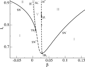
Figure 1: Phase diagram of DS in the nonlocal Kerr cavity for $\theta=1.23$. DS do not exist in Region I, below the saddle node line (SN). DS are stable between the saddle-node bifurcation (solid line - SN) and the Hopf bifurcation (dashed line - H), namely in Regions II, III, VI and VIII (see also Fig. 2). In Regions IV and VII delimited by a Hopf and a saddle-loop bifurcation (dotted line - SL) there are stable oscillatory DS while the stationary DS are unstable. In Region V the static DS is unstable and the phase space generated after the destruction of the limit cycle at the SL induces a regime of excitable DS. Region VI corresponds to a regime of conditional excitability with both stable and excitable DS. Finally in Region VIII one encounters tristability: a stationary and an oscillatory DS coexist with the homogeneous solution. Where the saddle-node bifurcation line and the Hopf bifurcation line meet is a Takens-Bogdanov (TB) bifurcation.

III.1 Preliminary remarks

In this section, we show the different possibilities of dynamical behavior of DS in parameter space (see Fig. 1). Since DS are radially symmetric they correspond to stationary solutions of the radial form of Eq. (1) with boundary conditions $\partial_{r}E(r=0)=0$ and $\partial_{r}E(r\rightarrow\infty)=0$. This equation can be solved numerically using a Newton method McSloy et al. (2002); Gomila et al. (2007); Gelens et al. (2007). This approach is very accurate and automatically generates the Jacobian operator, whose eigenvalues determine the stability of the solutions. Note that this method finds both stable and unstable stationary solutions. DS can undergo two kinds of instabilities, radial instabilities which preserve the localized character of the structure and azimuthal instabilities which lead to the formation of extended patterns. The last ones appear only for large values of the background intensity ($I_{s}$ close to 1). We focus here on the radial instabilities, so phase diagrams (Figs. 1 and 2) are plotted only up to $I_{s}=0.93$, before the azimuthal instabilities take place.

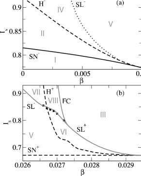
Figure 2: Zoom of Fig. 1 near TB₁ (a) and TB₂ (b). Lines have been determined using the method explained in Section III.1 with the exception of the SL line in panel (b). In that case the filled squares display the location of the SL obtained from numerical integration of Eq. (1), while the grey line through these points is only to guide the eye. $\theta$ = 1.23.

Since the system has three parameters ($I_{s}$, $\theta$, $\beta$), for the sake of clarity we fix the detuning at $\theta=1.23$ in this section and analyze a slice of the whole parameter space. Fig. 1 shows the region of the parameter plane $(\beta,I_{s})$ that contains the most relevant regimes of dynamical behavior of the system. The line that dominates this parameter plane has the shape of a deformed parabola, and is a line of saddle-node (SN) bifurcations in which two DS are created. Below this line one has Region I where no DS exist. We recall that in all the parameter range covered by Fig. 1 the spatially homogeneous solution is always stable. The different regimes above this line are organized by two codimension-$2$ Takens-Bogdanov points, TB₁ $(\beta=0.00987,I_{s}=0.7741)$ and TB₂ $(\beta=0.02944,I_{s}=0.6707)$, discussed in the next two Sections.

Without the bilaplacian term there is only one TB point Gomila et al. (2005, 2007). In that case, the TB point is found only asymptotically for the limit $\theta\rightarrow\infty$. As we will discuss later, that TB point corresponds in fact to the TB₁ point found here. Therefore, the nonlocality has brought this bifurcation to finite parameter values allowing us to fully study the different dynamical regimes around the TB₁ point.

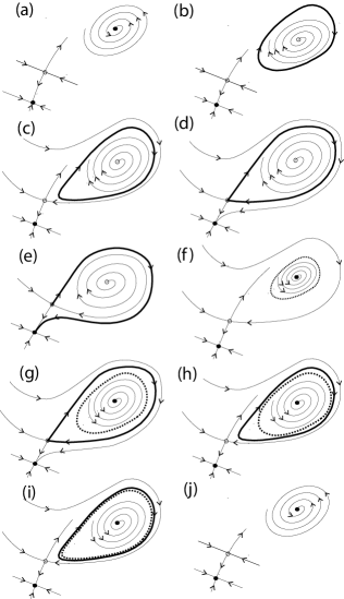
Figure 3: Qualitative evolution of the phase space at $I_{s}\approx 0.8$ and $\theta=1.23$ for increasing values of $\beta$, corresponding to the different dynamical behavior in a horizontal cut of Fig. 1. From (a) to (j), one goes from stable DS (Region II) to an oscillating DS (Region IV), followed by an excitable DS (Region V), a conditional excitable DS (Region VI), a coexistence of stable DS and oscillatory DS (Region VIII) and finally a stable DS (Region III).

III.2 Dynamical scenario around the TB₁ point

A Takens-Bogdanov (or double-zero) bifurcation is associated to the presence of two (non-diagonalizable) degenerate null eigenvalues Takens (1974); Bogdanov (1974). Such a bifurcation occurs when, in a line of SN bifurcations, one of the modes transverse to the center manifold (of the SN bifurcation) passes through zero, implying that this transverse mode switches from stable to unstable or vice versa. If this transverse mode is stable we will denote the SN bifurcation line as SN^-, while we use SN⁺ if this mode is unstable. Throughout the remainder of this paper, we will use ^- for bifurcations for which there is a stable emerging solution and ⁺ if the emerging solutions are unstable. H^- will describe a supercritical Hopf, and H⁺ a subcritical one.

Another feature of a TB point is that two new bifurcation lines emerge from it Kuznetsov (2004): a Hopf bifurcation line and a saddle-loop (homoclinic) bifurcation line . In order to specify whether the cycle that emerges from the saddle-loop bifurcation is stable or unstable, it is useful to define the saddle-quantity $\nu$. For low-dimensional dynamical systems this quantity is given by $\nu=\lambda_{s}+\lambda_{u}$, with $\lambda_{u}>0$ and $\lambda_{s}<0$ the unstable and stable eigenvalues of the saddle, respectively. The emerging cycle will be stable if $\nu<0$, and unstable in the opposite case: $\nu>0$ Kuznetsov (2004).

At the TB₁ point, the saddle-node bifurcation is stable (SN^-), the Hopf is supercritical (H^-), and the saddle-loop creates a stable cycle (SL^-). Along the SN^- line a pair of stationary DS are created, one stable (upper branch) and the other (middle branch) unstable along a single direction in phase space (thus, a saddle point in dynamical systems parlance). So, Region II is characterized by stable DS coexisting with the spatially homogeneous solution. A qualitative sketch of the most relevant different kinds of behavior in the system as $\beta$ is increased can be found in Fig. 3 (this corresponds to a horizontal line in Fig. 2 for $I_{s}\approx 0.8$). In this figure, panel (a) reflects the behavior inside Region II, where the DS is the stable focus, the homogeneous solution is the stable node and the middle branch DS is the saddle.

The upper branch DS solution becomes unstable at the supercritical Hopf bifurcation, H^-, and leads to Region IV, characterized by oscillatory DS, i.e., autonomous oscillons. Fig. 3 (b) illustrates the behavior past the Hopf bifurcation: the stable oscillatory DS and the unstable focus in the center can be seen. Approaching the SL^- line a saddle-loop (homoclinic) bifurcation takes place, in which the limit cycle (oscillatory DS) becomes a homoclinic orbit of the saddle (middle branch DS). The SL^- is a global bifurcation, and cannot be detected through a local analysis. Thus, in this study it has been determined through numerical simulations of Eq. (1). Panel (c) in Fig. 3 illustrates the cycle growing in amplitude and approaching the saddle, while in panel (d) the cycle has become the homoclinic orbit of the saddle. The approach of the stable cycle to the saddle can also be seen quantitatively in panel (a) of Fig. 4: in this figure bifurcation diagrams corresponding to vertical cuts in parameter space, i.e. with $\beta$ fixed (cf. Fig. 1), are presented. Beyond the SL^-, the behavior of the system is excitable (Region V) Gomila et al. (2005, 2007), in particular of type (or class) I Izhikevich (2000), as the excitability threshold is the stable manifold of the saddle. An excitable excursion is achieved when localized perturbations beyond this threshold are applied to the spatially homogeneous solution. Fig  3 (e) sketches the phase space in the excitable regime past the saddle-loop bifurcation.

Inside Region V, no stable DS are found, only unstable DS solutions exist, and the system is excitable for all values of $I_{s}$ above the SN⁺ line. This line which is just the continuation of SN^- past the TB₁ point was is not observed in Gomila et al. (2005, 2007) since the TB point without bilaplacian term is located at $\theta\rightarrow\infty$. The SN⁺ line creates a saddle-unstable node pair (middle and upper branch, respectively). The pair of unstable solutions can be seen in the bifurcation diagram shown in Fig. 4(b) corresponding to a vertical cut of the parameter plane just to the right of TB₁ point.

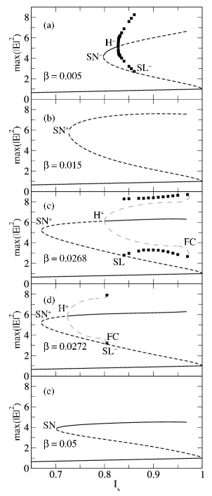
Figure 4: Bifurcation diagrams showing the maximum intensity of the DS as function of the background intensity $I_{s}$, for: (a) $\beta=0.005$; (b) $\beta=0.015$; (c) $\beta=0.0268$; (d) $\beta=0.0272$; (e) $\beta=0.05$. The lowest solid line represents the stable homogeneous solution. The lowest dashed line shows the maximum intensity of the unstable middle branch DS. Above that line, the upper branch DS is shown, where the solid line stands for the stable DS and the dashed line for the unstable DS. In (a), (c) and (d) the system exhibits stable oscillatory behavior (see text). In these cases, the maximum and minimum intensity of the oscillating DS are depicted as filled squares. The grey dashed line, representing the unstable limit cycle, is only a guiding line for the eye. When the limit cycle touches the middle branch DS, a saddle-loop bifurcation occurs. $\theta$ = 1.23.

III.3 Dynamical scenario around the TB₂ point

An even richer scenario is found around the TB₂ point. Comparing Fig. 2(a) and (b), one can see that the TB₂ does not yield the same scenario as around TB₁. In TB₁ the two lines that emerge involve stable objects (H^- and SL^- create and destroy, respectively, a stable limit cycle), while in TB₂ the Hopf line is subcritical (involving an unstable cycle). Furthermore, in the TB₁ point the two lines, H^- and SL^- are tangent to the line SN^- of stable saddle-node bifurcations while the opposite happens for TB₂ (the lines unfolding are tangent to SN⁺).

These differences correspond to a change of sign in a term of the normal form of the TB bifurcation Kuznetsov (2004):

$$\begin{array}[]{rcl}\dot{x}&=&y\\ \dot{y}&=&a+b\,x+\,x^{2}+s\,x\,y\ ,\quad s=\pm 1.\end{array}$$ (4)

The case that is most often discussed in the literature leads to the scenario discussed in Section III.2, and corresponds to $s=-1$. A supercritical Hopf line unfolds from the TB point tangent to the SN^- segment, and a saddle-loop, in which a stable cycle is destroyed unfolds tangent to the Hopf line. In the $s=+1$ case, however, a subcritical Hopf bifurcation line that creates an unstable cycle unfolds tangent to the SN⁺ segment, and the unstable cycle is destroyed in a saddle-loop also tangent to the Hopf bifurcation. This can be seen noticing that changing the sign of $s$ is equivalent to perform the substitutions $t\mapsto-t$ and $y\mapsto-y$. This scenario fits nicely with what is observed around the TB₂ point, and, thus, TB₁ and TB₂ correspond to the two possible cases of Eq. (4), with $s=-1$ and $s=+1$, respectively.

Crossing the H⁺ line coming from Region V, the unstable (upper branch) DS exhibits a subcritical Hopf bifurcation and becomes a stable focus. The cycle that is created is unstable and has only a single unstable direction. In Region VI the system is then bistable (upper branch DS and homogeneous solutions coexist) and the unstable cycle is the basin boundary of the upper branch stable DS as qualitatively illustrated in Fig. 3 (f). Just after the bifurcation this basin of attraction is small (since the initial cycle amplitude is zero) and grows as one moves away from the bifurcation line. This can be seen in the bifurcation diagram displayed in Fig. 4(c) corresponding to a vertical cut of Figs. 1 and 2 at $\beta=0.0268$. The upper branch DS becomes stable around $I_{s}=0.8$. The dashed grey line has been drawn with the purpose of guiding the eye only. It represents the unstable cycle that we do not compute. This bifurcation diagram also shows the existence of a stable limit cycle (plotted as squares) corresponding to an oscillatory DS. The stable limit cycle comes from a fold of cycles (FC) bifurcation, discussed in more detail later, which takes place at a larger value of $I_{s}$. Decreasing $I_{s}$ the stable limit cycle disappears at a saddle-loop bifurcation which takes place when the stable limit cycle becomes the homoclinic orbit of the saddle (middle branch soliton). In Fig. 4(c) Region VI corresponds to the values of $I_{s}$ limited on the left by the subcritical Hopf (H⁺) and the right by the saddle loop (SL⁺ and SL^-). Precise values for the SL^- obtained from numerical integration of Eq. (1) are plotted as filled squares in Fig. 2(b) while the grey SL line joining the points have been drawn to guide the eye. As we will discuss in the next subsection, Region VI corresponds to a regime of conditional excitability.

In Fig. 4(c), the FC on the one hand and the SL^- on the other limit a new region of tristability where a stationary DS, a oscillatory DS and the homogeneous solution coexist. In Fig. 2(b) the tristable region is labeled as VIII. In Fig. 3 the panel (g) sketches the phase space at the saddle-loop while the panel (h) illustrates the tristable regime. Increasing $\beta$ or $I_{s}$ in parameter space the stable cycle decreases in amplitude while the unstable limit cycle increases until both the stable and unstable cycles are destroyed in the fold bifurcation (Fig. 3(i)). Figure 5 shows the time evolution in the tristable regime obtained starting from an initial condition belonging to the basin of attraction of the limit cycle and from an initial condition within the basin of attraction of the stable DS.

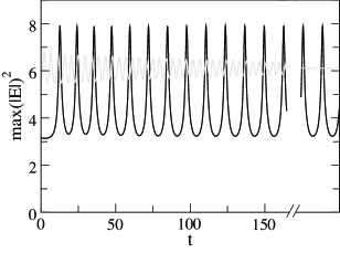
Figure 5: Dynamical evolution of the system in the tristable regime, where the spatially homogeneous fundamental branch (not shown), stable oscillatory DS regime (solid line), and stable focus (gray line) coexists.

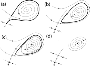
Figure 6: A qualitative sketch of the phase space at $I_{s}\approx 0.9$ and $\theta=1.23$ for increasing values of $\beta$, corresponding to a horizontal cut of Fig. 2(b), is depicted in Fig. 6. Increasing $\beta$ from (a) to (d), one starts with excitable DS (Region V), going through a region of bistability between a stable limit cycle and the stable homogeneous solution (Region VII), followed by a coexistence of stable DS and oscillatory DS (Region VIII) and finally a stable DS (Region III).

In the phase diagram (Fig. 2(b)) the SL^- line can also be located to the left of H⁺ (Region VII). The bifurcation diagram in this case would be similar to the one shown in Fig. 4(c), except for the fact that the SL^- becomes a SL⁺ and the H⁺ takes place at a larger value of $I_{s}$ than the SL^-. Therefore VII is a region of bistability where a stable limit cycle corresponding to the oscillatory upper branch DS coexist with the homogeneous solution while the steady state upper branch DS is an unstable focus. A qualitative sketch of the phase space when going from region V through VII and VIII is depicted in Fig. 6.

The last region in the phase diagram to be described is Region III, located to the right of the SL⁺ and FC lines. The phase space corresponding to this broad region is sketched in Figs. 3(j) and 6(d). The upper branch stationary DS is a stable point and coexists with the homogeneous solution. Fig. 4(e) shows a quantitative bifurcation diagram corresponding to a vertical cut of Fig. 1 for $\beta=0.05$, to the right of the TB₂. For $I_{s}<0.7$ only the homogeneous solution exists (Region I) while above $I_{s}=0.7$ one enters in Region III of coexistence of the stable DS with the homogeneous solution.

We now analyze in detail the fold of limit cycles bifurcation. It appears at a secondary codimension-2 point named resonant side-switching, where the fold and the saddle-loop bifurcation, that delimit the region of tristability, coalesce Chow et al. (1990); Champneys and Kuznetsov (1994). This occurs, roughly, around $\beta=0.0272$ and $I_{s}=0.82$. Fig. 4(d) depicts a bifurcation diagram close to this codimension-2 point, for which the region of existence of stable limit cycles is quite narrow: the represented square is very close both to the saddle-loop bifurcation and to the fold of cycles. In the phase diagram shown in Fig. 2(b) this codimension-2 corresponds to the point where the FC and the SL (SL^- and SL⁺) lines meet.

The occurrence of the resonant side-switching bifurcation is related to the eigenvalue spectrum of the saddle, namely, the saddle quantity of the middle branch DS approaches zero, and the cycle emerging from the saddle-loop changes from ”stable” to ”unstable”. Close to TB₂ point the saddle-loop bifurcation must destroy an unstable cycle (transition from Region VI to III), hence $\nu>0$, while after the fold has taken place it destroys a stable cycle (transition from Region VIII to VI), so $\nu<0$. Fig. 7 shows the spectrum of the middle branch DS for two different sets of parameters, one after the formation of the fold (saddle-loop bifurcation with a stable cycle, top panel) and one very close to the TB₂ point (saddle-loop bifurcation with an unstable cycle, bottom panel). The eigenvalues of the modes relevant for the dynamics are highlighted with filled circles, and indeed, the saddle quantity is positive $\nu>0$, albeit quite small ($\nu\sim 0.003$) in the bottom panel, compatible with the fact that it involves an unstable cycle. One can observe that close to the SL⁺ that emerges from the TB₂ point, where the saddle quantity is positive, four localized modes play a role in the dynamical behavior of the system. However, when moving away from the SL⁺ line, only two localized modes determining the dynamics remain. So, in conclusion, we can say that the system is essentially two-dimensional for the same reasons as discussed in Ref. Gomila et al. (2007), except close to the SL⁺ line, originating from the TB₂ point.

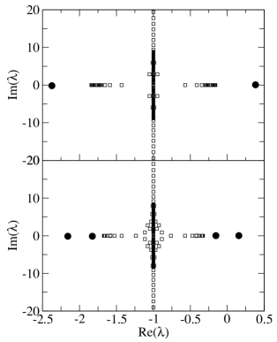
Figure 7: The spectrum of the middle-branch DS at the saddle-loop bifurcation for (a) $\beta=0.0268$ and $I_{s}=0.84$, and (b) $\beta=0.0294$ and $I_{s}=0.671$. The filled black circles are the eigenvalues corresponding to the modes with a localized spatial profile. $\theta=1.23$.

III.4 Excitability and conditional excitability

When crossing a saddle-loop bifurcation from a region where a stable oscillatory DS exist one enters in a excitable regime. As discussed in Subsection III.2, this scenario takes place when going from Region IV (where the oscillatory DS is stable) to Region V where DS exhibit excitability. Of course it is also possible to enter in Region V from the other side, namely from the side of the TB₂ point. In fact a similar scenario is found when going from Region VII where the oscillatory DS is stable to Region V. In any case the stable manifold of the saddle (middle branch DS) plays the role of excitability threshold, so the excitable response is triggered only by localized perturbations of the homogeneous solution that bring the system beyond this threshold. Excitability is of Class I Izhikevich (2000), characterized by long response times for perturbations that leave the trajectory close to the saddle in phase space.

Close to the TB₂ point there is another region, VI, where one can enter crossing a saddle-loop line. However, the dynamical behavior in Region VI is qualitatively different from Region V since the upper branch LS is an unstable focus in the last one, while it is stable in the former. As discussed before, the upper branch LS has been made stable by the subcritical Hopf bifurcation H⁺ that separates Region V from VI. The H⁺ bifurcation generates also an unstable limit cycle, which is not present in Region V. Therefore, although the transition from Regions III or VIII to Region VI goes through a saddle-loop bifurcation, the scenario must be qualitatively different from the one discussed above which leads to the usual excitability found in Region V. In Region VI, one finds a regime of conditional excitability, in which the DS is simultaneously excitable and bistable. The excitable behavior is also Class I.

To clarify what conditional excitability means, we refer to the phase space sketched in Fig. 3(f). In this situation, while as usual, perturbations of the homogeneous solution that are not able to cross the excitability threshold (stable manifold of the saddle) lead to normal relaxation, there are two possible different dynamical responses for supra-threshold perturbations. If a localized perturbation of the homogeneous state brings the system inside the basin of attraction of the stable focus, namely inside the unstable cycle, the system jumps from the fundamental solution to this attractor. Therefore after this perturbation the system relaxes to the stable DS in a oscillatory way. The grey line in Fig. 8 shows the dynamical evolution of the maxima of the peak in this situation. Instead, for localized perturbations of the homogeneous solution which bring the system beyond the stable manifold of the saddle but outside the unstable cycle, the response is excitable. The system exhibits a large response corresponding to a circulation around the unstable limit cycle before returning to the stable homogeneous solution. The black line in Fig. 8 shows the time evolution of maxima of the peak for a excitable trajectory.

So, in summary, the dynamical response of perturbations is more complex than simply sub- and supra-threshold, and for the latter type of perturbations two possible regimes are possible. When going from Region VI to Region V at the H⁺ line, the upper branch DS becomes unstable and the unstable limit cycle responsible for the conditional excitable response to supra-threshold perturbations disappears, so the conditional excitability becomes a usual one.

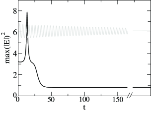
Figure 8: The conditional excitability regime is illustrated for $\beta=0.0272$ and $I_{s}=0.8$. The solid line (excitable trajectory) corresponds to time evolution of the maxima of the peak after a localized perturbation of the homogeneous state that brings the system beyond the excitability threshold but outside the basin of attraction of the upper branch DS. The grey line corresponds to a stronger localized perturbation that brings the system inside the boundary of attraction of the upper branch DS.

IV Concluding Remarks

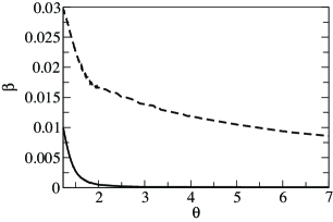
Figure 9: Location ($\theta_{TB},$$\beta_{TB}$) of the two TB points as the detuning is increased. The solid line and the dashed line correspond to the TB₁ and TB₂ point, respectively.

We have studied the nonlinear dynamical behavior of 2D localized structures in a model for an optical cavity filled by a Kerr nonlinear medium and a left-handed metamaterial Gelens et al. (2007). The model is a generalization of the Lugiato-Lefever equation Lugiato and Lefever (1987), and includes higher order spatial effects arising from the weakly nonlocal response of the metamaterial. In this system, we have shown the existence of regions with stationary, oscillating and excitable localized structures. Furthermore, we have shown that the different bifurcation lines originate from two Takens-Bogdanov (TB) codimension-2 points, which is a strong signature for the presence of a homoclinic bifurcation. This homoclinic bifurcation offers a route to excitable behavior of the 2D localized structures. Finally an extra secondary codimension-2 point (resonant side-switching bifurcation) creates a fold of cycles that leads to two new regimes, one of tristability and one of conditional excitability.

Without the nonlocal terms the different dynamical regimes of the DS were organized by a TB point located at the limit of infinite detuning, where the Lugiato-Lefever equation reduces to the (conservative) Nonlinear Schrödinger Equation (NLSE) Gomila et al. (2005, 2007). Here, we demonstrate that the presence of higher order spatial effects brings two TB points to finite parameter values. In Fig. 9, we provide further evidence that TB₁ is unfolding from the NLSE at the limit $\beta\rightarrow 0$ and then $\theta\rightarrow\infty$ of Eq. (1). This hypothesis is supported by the fact that 2D solitons in the NLSE have at least a twofold degeneracy Skryabin (2002). Furthermore, Fig. 9 also gives some evidence that TB₂ comes from a certain conservative limit at $\theta\rightarrow\infty$, $\beta\rightarrow 0$ of Eq. (1). However, if this is a singular limit, this does not necessarily imply that TB₁ and TB₂ have to evolve towards the same point in the conservative limit. The numerical evidence given in Fig. 9 is of course not fully conclusive, and this unfolding of both of the TB points is presently under investigation.