Phase portraits for quadratic homogeneous polynomial vector fields on $\mathbb{S}^{2}$

Jaume Llibre and Claudio Pessoa

Departament de Matemàtiques, Universitat Autònoma de Barcelona

08193 Bellaterra, Barcelona, Spain

Abstract. Let $X$ be a homogeneous polynomial vector field of degree $2$ on $\mathbb{S}^{2}$. We show that if $X$ has at least a non–hyperbolic singularity, then it has no limit cycles. We give necessary and sufficient conditions for determining if a singularity of $X$ on $\mathbb{S}^{2}$ is a center and we characterize the global phase portrait of $X$ modulo limit cycles. We also study the Hopf bifurcation of $X$ and we reduce the $16^{th}$ Hilbert’s problem restricted to this class of polynomial vector fields to the study of two particular families. Moreover, we present two criteria for studying the nonexistence of periodic orbits for homogeneous polynomial vector fields on $\mathbb{S}^{2}$ of degree $n$.

1. Introduction and statement of the main results

A polynomial vector field $X$ in $\mathbb{R}^{3}$ is a vector field of the form

(1) $$X=P(x,y,z)\frac{\partial}{\partial x}+Q(x,y,z)\frac{\partial}{\partial y}+R(x,y,z)\frac{\partial}{\partial z},$$

where $P$, $Q$ and $R$ are polynomials in the variables $x$, $y$ and $z$ with real coefficients. We denote $n=\max\{\deg P,\deg Q,\deg R\}$ the degree of the polynomial vector field $X$. In what follows $X$ will denote the above polynomial vector field.

Let $\mathbb{S}^{2}$ be the $2$–dimensional sphere $\{(x,y,z)\in\mathbb{R}^{3}\;:x^{2}+y^{2}+z^{2}=1\}$. A polynomial vector field $X$ on $\mathbb{S}^{2}$ is a polynomial vector field in $\mathbb{R}^{3}$ such that restricted to the sphere $\mathbb{S}^{2}$ defines a vector field on $\mathbb{S}^{2}$; i.e. it must satisfy the equality

(2) $$xP(x,y,z)+yQ(x,y,z)+zR(x,y,z)=0,$$

for all points $(x,y,z)$ of the sphere $\mathbb{S}^{2}$.

Let $f\in\mathbb{R}[x,y,z]$, where $\mathbb{R}[x,y,z]$ denotes the ring of all polynomials in the variables $x$, $y$ and $z$ with real coefficients. The algebraic surface $f=0$ is an invariant algebraic surface of the polynomial vector field $X$ if for some polynomial $K\in\mathbb{R}[x,y,z]$ we have $\displaystyle Xf=P\frac{\partial f}{\partial x}+Q\frac{\partial f}{\partial y}+R\frac{\partial f}{\partial z}=Kf$. The polynomial $K$ is called the cofactor of the invariant algebraic surface $f=0$. We note that since the polynomial system has degree $n$, then any cofactor has at most degree $n-1$.

The algebraic surface $f=0$ defines an invariant algebraic curve $\{f=0\}\cap\mathbb{S}^{2}$ of the polynomial vector field $X$ on the sphere $\mathbb{S}^{2}$ if

• for some polynomial $K\in\mathbb{R}[x,y,z]$ we have $\displaystyle Xf=P\frac{\partial f}{\partial x}+Q\frac{\partial f}{\partial y}+R\frac{\partial f}{\partial z}=Kf$, on all the points $(x,y,z)$ of the sphere $\mathbb{S}^{2}$, and

• the intersection of the two surfaces $f=0$ and $\mathbb{S}^{2}$ is transversal; i.e. for all points $(x,y,z)\in\{f=0\}\cap\mathbb{S}^{2}$ we have that $\displaystyle(x,y,z)\land\left(\frac{\partial f}{\partial x},\frac{\partial f}{\partial y},\frac{\partial f}{\partial z}\right)\neq 0$, where $\land$ denotes the vector cross product in $\mathbb{R}^{3}$.

Again the polynomial $K$ is called the cofactor of the invariant algebraic curve $\{f=0\}\cap\mathbb{S}^{2}$.

Note that, if a curve $\{f=0\}\cap\mathbb{S}^{2}$ satisfies the above definition, then it is formed by trajectories of the vector field $X$. This justifies to call $\{f=0\}\cap\mathbb{S}^{2}$ an invariant algebraic curve, since in this case it is invariant under flow defined by $X$ on $\mathbb{S}^{2}$.

The equation of a plane in $\mathbb{R}^{3}$ is given for $ax+by+cz+d=0$. Any circle on the sphere lies in a plane $ax+by+cz+d=0$, where we can assume that $a^{2}+b^{2}+c^{2}=1$ and $0\leq-d<1$. If the invariant algebraic curve $\{f=0\}\cap\mathbb{S}^{2}$ is contained in some plane, then we say that $\{f=0\}\cap\mathbb{S}^{2}$ is an invariant circle of the polynomial vector field $X$ on the sphere $\mathbb{S}^{2}$. Moreover, if the plane contains the origin, then $\{f=0\}\cap\mathbb{S}^{2}$ is an invariant great circle.

Let $U$ be an open subset of $\mathbb{R}^{3}$. Here a nonconstant analytic function $H:U\rightarrow\mathbb{R}$ is called a first integral of the system on $U$ if it is constant on all solutions curves $(x(t),y(t),z(t))$ of the vector field $X$ on $U$; i.e. $H(x(t),y(t),z(t))=$ constant for all values of $t$ for which the solution $(x(t),y(t),z(t))$ is defined in $U$. Clearly $H$ is a first integral of the vector field $X$ on $U$ if and only if $XH\equiv 0$ on $U$. If $X$ is a vector field on $\mathbb{S}^{2}$, the definition of first integral on $\mathbb{S}^{2}$ is the same substituting $U$ by $U\cap\mathbb{S}^{2}$.

In what follows we say that two phase portraits of the vector fields $X_{1}$ and $X_{2}$ on $\mathbb{S}^{2}$ are (topologically ) equivalent, if there exists a homeomorphism $h:\mathbb{S}^{2}\rightarrow\mathbb{S}^{2}$ such that $h$ applies orbits of $X_{1}$ into orbits of $X_{2}$, preserving or reversing the orientation of all orbits. Similarly we define (topological) equivalence in the Poincaré disc, see Section 2 for a definition.

In [11] we studied homogeneous polynomial vector fields of degree $2$ on $\mathbb{S}^{2}$, and we determined the maximum number of invariant circles when it has finitely many invariant circles. Moreover, we characterized the global phase portraits of these vector fields when they have finitely many invariant circles. Camacho [2] in $1981$ proved some properties of this kind of vector fields, see also [10]. One of the results that can be found in [11] and that will be necessary in this paper is given below.

Proposition 1.

Let $X$ be a homogeneous polynomial vector field of degree $2$ on $\mathbb{R}^{3}$. Then $X$ is a polynomial vector field on $\mathbb{S}^{2}$ if and only if the system associated to it can be written as

(3) $$\begin{array}[]{lcl}\dot{x}&=&P(x,y,z)=a_{1}xy+a_{2}y^{2}+a_{3}z^{2}+a_{4}xz+a_{5}yz,\\ \dot{y}&=&Q(x,y,z)=-a_{1}x^{2}-a_{2}xy+a_{6}z^{2}+a_{7}xz+a_{8}yz,\\ \dot{z}&=&R(x,y,z)=-a_{4}x^{2}-a_{8}y^{2}-(a_{5}+a_{7})xy-a_{3}xz-a_{6}yz.\end{array}$$

The main results of this paper are the following ones.

The next theorem characterizes the centers of the quadratic homogeneous polynomial vector fields on $\mathbb{S}^{2}$.

Theorem 2.

Let $X$ be a homogeneous polynomial vector field on $\mathbb{S}^{2}$ of degree $2$ and let $p=(0,0,-1)$ be a singularity of $X$; i.e. the system associated to $X$ can be written in the form (3) with $a_{3}=a_{6}=0$. Then $p$ is a center of $X$ if and only if $a_{8}=-a_{4}$, $a_{4}^{2}+a_{7}a_{5}<0$ and $a_{4}(a_{1}^{2}-a_{2}^{2})+a_{1}a_{2}(a_{5}+a_{7})=0$.

Theorem 2 will be proved in Section 4.

In the next two results we provide sufficient conditions for the non–existence of periodic orbits (and in particular of limit cycles) for homogeneous polynomial vector fields on $\mathbb{S}^{2}$ of arbitrary degree. For more details on limit cycles see [13].

We use the notation $\tilde{F}(u,v)=F(2u,2v,u^{2}+v^{2}-1)$, where $F\in\mathbb{R}[x,y,z]$.

Theorem 3.

Let $X=(P,Q,R)$ be a homogeneous polynomial vector field on $\mathbb{S}^{2}$. Then $X$ has no periodic orbits if at least one of following conditions is satisfied.

• The polynomial $\tilde{R}$ does not change sign on $\mathbb{R}^{2}$ and $X$ does not have a periodic orbit passing through the point $(0,0,1)$.

• The function $\langle(\tilde{P},\tilde{Q}),\nabla\tilde{R}\rangle\mid_{\tilde{R}=0}$ does not change sign and $X$ does not have a periodic orbit passing through the point $(0,0,1)$.

Now, we use the notation $\mathcal{K}=aP+bQ+cR$, $\tilde{F}_{1}(u,v)=F(u+a,v+b,c-(au+bv)/c)$, $\tilde{F}_{2}(u,v)=F(a-(bu+cv)/a,u+b,v+c)$ and $\tilde{F}_{3}(u,v)=F(u+a,b-(au+cv)/b,v+c)$ and $F\in\mathbb{R}[x,y,z]$.

Theorem 4.

Suppose that the homogeneous polynomial vector field $X=(P,Q,R)$ does not have periodic orbits on $\mathbb{S}^{2}$ intersecting the great circle $C$ determined by plane $ax+by+cz=0$ with $a^{2}+b^{2}+c^{2}=1$. Then it has no periodic orbits if at least one of following conditions is satisfied.

• The polynomial $\tilde{\mathcal{K}}_{1}$ does not change sign on $\mathbb{R}^{2}$.

• The function $\langle(\tilde{P}_{1},\tilde{Q}_{1}),\nabla\tilde{\mathcal{K}}_{1}\rangle\mid_{\tilde{\mathcal{K}}_{1}=0}$ does not change sign.

• The polynomial $\tilde{\mathcal{K}}_{2}$ does not change sign on $\mathbb{R}^{2}$.

• The function $\langle(\tilde{Q}_{2},\tilde{R}_{2}),\nabla\tilde{\mathcal{K}}_{2}\rangle\mid_{\tilde{\mathcal{K}}_{2}=0}$ does not change sign.

• The polynomial $\tilde{\mathcal{K}}_{3}$ does not change sign on $\mathbb{R}^{2}$.

• The function $\langle(\tilde{P}_{3},\tilde{R}_{3}),\nabla\tilde{\mathcal{K}}_{3}\rangle\mid_{\tilde{\mathcal{K}}_{3}=0}$ does not change sign.

Theorems 3 and 4 will be proved in Section 5.

The following theorem characterizes the phase portraits of quadratic homogeneous polynomial vector fields on $\mathbb{S}^{2}$ having at least one non–hyperbolic singularity.

Theorem 5.

Let $X$ be a homogeneous polynomial vector field on $\mathbb{S}^{2}$ of degree $2$.

• If $X$ has a linearly zero singularity, then its phase portrait is equivalent to the phase portrait of Figure 1.

• If $X$ has a nilpotent singularity, then its phase portrait in the Poincaré disc is equivalent to one of the phase portraits of Figures 2 or 3.

• If $X$ has a center, then its phase portrait in the Poincaré disc is equivalent to one of the phase portraits of Figures 5 or 6.

• If $X$ has a semi–hyperbolic singularity, then its phase portrait in the Poincaré disc is equivalent to one of the phase portraits of Figures 7 or 8.

We note that the unique non–hyperbolic singularity which does not appear explicitly in the statement of Theorem 5 is a weak focus. Such singularities can appear in the quadratic homogeneous polynomial vector fields on $\mathbb{S}^{2}$ and such vector fields are studied in Theorems 8 and 9. Hence, from Theorem 5 it follows immediately.

Corollary 6.

Let $X$ be a homogeneous polynomial vector field on $\mathbb{S}^{2}$ of degree $2$. If $X$ has at least a non–hyperbolic singularity on $\mathbb{S}^{2}$ different from a weak focus, then $X$ has no limit cycles on $\mathbb{S}^{2}$.

Theorem 5 and Corollary 6 will be proved in Section 6.

In the next theorem we give an upper bound for the number of singularities of homogeneous polynomial vector fields on $\mathbb{S}^{2}$ of arbitrary degree.

Theorem 7.

Let $X=(P,Q,R)$ be a homogeneous polynomial vector field on $\mathbb{S}^{2}$ of degree $n$. If $X$ has finitely many singularities on $\mathbb{S}^{2}$, then $X$ has at most $2(n^{2}-n+1)$ singularities on $\mathbb{S}^{2}$.

Theorem 7 will be proved in Section 7.

The following theorem characterize modulo limit cycles the phase portraits of quadratic homogeneous polynomial vector fields on $\mathbb{S}^{2}$ having non–degenerate singularities.

Theorem 8.

Let $X$ be a homogenous polynomial vector field on $\mathbb{S}^{2}$ of degree $2$. If all singularities of $X$ are non–degenerate, then its phase portrait in the Poincaré disc is topologically equivalent modulo limit cycles to one of the phase portraits giving in Figures 13.

Theorem 8 will be proved in Section 8.

The next result characterizes the families of quadratic homogeneous polynomial vector fields on $\mathbb{S}^{2}$ having a Hopf bifurcation.

Theorem 9.

Let $X$ be a family of homogeneous polynomial vector fields on $\mathbb{S}^{2}$ of degree $2$ having a Hopf bifurcation. Then, doing a orthogonal linear change of variables, the system associated to $X$ can be written as

$$\begin{array}[]{lcl}\dot{x}&=&a_{1}xy+a_{2}y^{2}+a_{5}yz,\\ \dot{y}&=&-a_{1}x^{2}-a_{2}xy+a_{7}xz+a_{8}yz,\\ \dot{z}&=&-(a_{5}+a_{7})xy-a_{8}y^{2},\end{array}$$

with $a_{1}\neq 0$, $a_{2}(a_{5}+a_{7})-a_{1}a_{8}\neq 0$ and $-a_{5}a_{7}<0$.

Theorem 9 will be proved in Section 9.

We have reduced the possible existence of limit cycles to two families; more precisely, the families (38) and (40). In Theorem 9 we have proved that family (40) has for some values of the parameters limit cycles. Finally in the last section we conjecture that family (38) has no limit cycles.

2. Poincaré disc

Let $X$ be a homogeneous polynomial vector field on $\mathbb{S}^{2}$, then the differential system associated to it is invariant with respect to the change of variables $(x,y,z,t)\mapsto(-x,-y,-z,-t)$ if its degree is even, or with respect to $(x,y,z,t)\mapsto(-x,-y,-z,t)$ if its degree is odd. Thus, in particular the phase portrait of $X$ at the northern hemisphere of $\mathbb{S}^{2}$ is symmetric with respect to the origin of the sphere to the phase portrait at the southern hemisphere with the time reverse if the degree of $X$ is even, or with the same time if the degree of $X$ is odd. We now project the northern hemisphere of $\mathbb{S}^{2}$ orthogonally onto the plane $\Pi$ containing the equator of $\mathbb{S}^{2}$, i.e. $\mathbb{S}^{1}$. The orbits of $X$ on the northern hemisphere of $\mathbb{S}^{2}$ are mapped onto certain curves of the unit disc of $\Pi$. We call this unit disc, together with the corresponding induced phase portrait, the Poincaré disc.

Now we consider the homogeneous polynomial vector field $X=(P,Q,R)$ of degree $m$. We identify $\mathbb{R}^{2}$ as the tangent plane to the sphere $\mathbb{S}^{2}$ at the point $p=(a,b,c)$, i.e with the plane $ax+by+cz-1=0$, where $a^{2}+b^{2}+c^{2}=1$. Suppose that $c\neq 0$, then we denote the points of $\mathbb{R}^{2}$ as $(u+a,v+b,c-(au+bv)/c)$. Let $\pi:\mathbb{R}^{2}\rightarrow\mathbb{S}^{2}\cap\{ax+by+cz>0\}$ be the diffeomorphism given by $\pi(u,v)=|c|/\sqrt{\lambda}\left(x=u+a,\;y=v+b,\;z=c-(au+bv)/c\right)$, where $\lambda=c^{2}(1+u^{2}+v^{2})+(au+bv)^{2}$. That is, $\pi$ is the inverse map of the central projection $\pi^{-1}:\mathbb{S}^{2}\cap\{ax+by+cz>0\}\rightarrow\mathbb{R}^{2}$ defined by

(4) $$\pi^{-1}(x,y,z)=\left(u=\frac{x}{ax+by+cz},\;v=\frac{y}{ax+by+cz},\frac{z}{ax+by+cz}\right).$$

The homogeneous polynomial system $X$ on $\mathbb{S}^{2}$ becomes, through the central projection $\pi^{-1}$, the differential system

$$\begin{array}[]{lcl}\dot{u}&=&\displaystyle\frac{\sqrt{\lambda}}{|c|}(\bar{P}-(u+a)(a\bar{P}+b\bar{Q}+c\bar{R})),\\ \dot{v}&=&\displaystyle\frac{\sqrt{\lambda}}{|c|}(\bar{Q}-(v+b)(a\bar{P}+b\bar{Q}+c\bar{R})),\end{array}$$

on the plane $\mathbb{R}^{2}$. Here $\displaystyle\bar{F}=F\left(\pi(u,v)\right)$. Since $X$ is a homogeneous polynomial vector field of degree $m$ we have that

$$\begin{array}[]{lcl}\dot{u}&=&\displaystyle\left(\frac{|c|}{\sqrt{\lambda}}\right)^{m-1}\left(\tilde{P}-(u+a)(a\tilde{P}+b\tilde{Q}+c\tilde{R})\right),\\ \dot{v}&=&\displaystyle\left(\frac{|c|}{\sqrt{\lambda}}\right)^{m-1}\left(\tilde{Q}-(v+b)(a\tilde{P}+b\tilde{Q}+c\tilde{R})\right),\end{array}$$

where $\tilde{F}=F(u+a,v+b,c-(au+bv)/c)$. If $t$ denotes the independent variable in the above differential system, then this system becomes polynomial introducing the new independent variable $s$ through $ds=(\sqrt{\lambda}/|c|)^{1-m}dt$, i.e.

(5) $$\begin{array}[]{lcl}\dot{u}&=&\mathcal{P}(u,v)=\displaystyle\tilde{P}-(u+a)(a\tilde{P}+b\tilde{Q}+c\tilde{R}),\\ \dot{v}&=&\mathcal{Q}(u,v)=\displaystyle\tilde{Q}-(v+b)(a\tilde{P}+b\tilde{Q}+c\tilde{R}).\end{array}$$

Now in the case $a\neq 0$ the central projection (4) induces a polynomial vector field on the plane $ax+by+cz-1=0$ determined by

(6) $$\begin{array}[]{lcl}\dot{u}&=&\mathcal{P}(u,v)=\displaystyle\tilde{Q}-(u+b)(a\tilde{P}+b\tilde{Q}+c\tilde{R}),\\ \dot{v}&=&\mathcal{Q}(u,v)=\displaystyle\tilde{R}-(v+c)(a\tilde{P}+b\tilde{Q}+c\tilde{R}),\end{array}$$

where $\tilde{F}=F(a-(bu+cv)/a,u+b,v+c)$; and in the case $b\neq 0$ we obtain

(7) $$\begin{array}[]{lcl}\dot{u}&=&\mathcal{P}(u,v)=\displaystyle\tilde{P}-(u+a)(a\tilde{P}+b\tilde{Q}+c\tilde{R}),\\ \dot{v}&=&\mathcal{Q}(u,v)=\displaystyle\tilde{R}-(v+c)(a\tilde{P}+b\tilde{Q}+c\tilde{R}),\end{array}$$

where $\tilde{F}=F(u+a,b-(au+cv)/b,v+c)$.

The proof of the next two propositions can be found in [17].

Proposition 10.

Let $X=(P,Q,R)$ be a homogeneous polynomial vector field of degree $m$ on $\mathbb{S}^{2}$. Then the planar vector field induced from $X$ through the central projection (4) on the plane $ax+by+cz-1=0$ with $a^{2}+b^{2}+c^{2}=1$ has degree $m$ if and only if the great circle $\{ax+by+cz=0\}\cap\mathbb{S}^{2}$ is an invariant circle of $X$.

In general we will consider the case $(a,b,c)=(0,0,-1)$. Thus (5) becomes

(8) $$\begin{array}[]{lcl}\dot{u}&=&\mathcal{P}(u,v)=\displaystyle P(u,v,-1)+uR(u,v,-1),\\ \dot{v}&=&\mathcal{Q}(u,v)=\displaystyle Q(u,v,-1)+vR(u,v,-1).\end{array}$$

In particular if $X$ is a homogeneous polynomial vector field on $\mathbb{S}^{2}$ of degree $2$ associated to (3), then (8) becomes

(9) $$\begin{array}[]{lcl}\dot{u}&=&a_{3}-a_{4}u-a_{5}v+a_{3}u^{2}+(a_{1}+a_{6})uv+a_{2}v^{2}\\ &&-a_{4}u^{3}-(a_{5}+a_{7})u^{2}v-a_{8}uv^{2},\\ \dot{v}&=&a_{6}-a_{7}u-a_{8}v-a_{1}u^{2}+(a_{3}-a_{2})uv+a_{6}v^{2}-\\ &&a_{4}u^{2}v-(a_{5}+a_{7})uv^{2}-a_{8}v^{3}.\end{array}$$

Proposition 11.

Let $X$ be a homogeneous polynomial vector field on $\mathbb{S}^{2}$ of degree $m$, and let $f\in\mathbb{R}[x,y,z]$ be a homogeneous polynomial of degree $n$ such that $f(x,y,0)\not\equiv 0$. Then $f=0$ is an invariant algebraic surface of $X$ if and only if $f(u,v,-1)=0$ is an invariant algebraic curve of the polynomial planar vector field given by (8) induced from $X$ through the central projection (4).

The next results jointly with their respective proofs can be found in Camacho [2] or in [17].

Proposition 12.

Let $X$ be the vector field associated to (3), and let $s_{1}$, $-s_{1}\in\mathbb{S}^{2}$ be saddle points of $X$ with a common separatrix $l$, then $l$ is contained in a great circle passing through $s_{1}$ and $-s_{1}$.

3. Stereographic projection

We identify $\mathbb{R}^{2}$ as the plane $ax+by+cz=0$ with $a^{2}+b^{2}+c^{2}=1$. Suppose that $c\neq 0$, then we denote the points of $\mathbb{R}^{2}$ as $(u,v,-(au+bv)/c)$. Let $\pi:\mathbb{R}^{2}\rightarrow\mathbb{S}^{2}\setminus\{(a,b,c)\}$ be the diffeomorphism given by $\pi(u,v)=1/\lambda(x=a\lambda-2c^{2}(a-u),\;y=b\lambda-2c^{2}(b-v),\;z=c\lambda-2c(c^{2}+au+bv))$, where $\lambda=c^{2}(1+u^{2}+v^{2})+(au+bv)^{2}$. That is, $\pi$ is the inverse map of the stereographic projection $\pi^{-1}:\mathbb{S}^{2}\setminus\{(a,b,c)\}\rightarrow\mathbb{R}^{2}$ defined by $\pi^{-1}(x,y,z)=$

(10) $$\left(u=\frac{x-a(ax+by+cz)}{1-(ax+by+cz)},\;v=\frac{y-b(ax+by+cz)}{1-(ax+by+cz)},\frac{z-c(ax+by+cz)}{1-(ax+by+cz)}\right).$$

Through the stereographic projection $\pi^{-1}$ the homogeneous polynomial system $X$ on $\mathbb{S}^{2}$ becomes the differential system

$$\begin{array}[]{lcl}\dot{u}&=&\displaystyle\frac{\lambda}{2c^{2}}(\bar{P}+(u-a)(a\bar{P}+b\bar{Q}+c\bar{R})),\\ \dot{v}&=&\displaystyle\frac{\lambda}{2c^{2}}(\bar{Q}+(v-b)(a\bar{P}+b\bar{Q}+c\bar{R})),\end{array}$$

on the plane $\mathbb{R}^{2}$. Here $\displaystyle\bar{F}=F\left(\pi(u,v)\right)$. Since $X$ is a homogeneous polynomial vector field of degree $m$ we have that

$$\begin{array}[]{lcl}\dot{u}&=&\displaystyle\frac{1}{2c^{2}\lambda^{m-1}}\left(\tilde{P}+(u-a)(a\tilde{P}+b\tilde{Q}+c\tilde{R})\right),\\ \dot{v}&=&\displaystyle\frac{1}{2c^{2}\lambda^{m-1}}\left(\tilde{Q}+(v-b)(a\tilde{P}+b\tilde{Q}+c\tilde{R})\right),\end{array}$$

where $\tilde{F}=F(a\lambda-2c^{2}(a-u),b\lambda-2c^{2}(b-v),c\lambda-2c(c^{2}+au+bv))$. If $t$ denotes the independent variable in the above differential system, then this system becomes polynomial introducing the new independent variable $s$ through $ds=\lambda^{1-m}/(2c^{2})dt$, i.e.

(11) $$\begin{array}[]{lcl}\dot{u}&=&\mathcal{P}(u,v)=\displaystyle\tilde{P}+(u-a)(a\tilde{P}+b\tilde{Q}+c\tilde{R}),\\ \dot{v}&=&\mathcal{Q}(u,v)=\displaystyle\tilde{Q}+(v-b)(a\tilde{P}+b\tilde{Q}+c\tilde{R}).\end{array}$$

Now the dot denotes derivative with respect to the variable $s$. In the cases $a\neq 0$ the stereographic projection (10) induces a polynomial vector field on the plane $ax+by+cz=0$ determined by

(12) $$\begin{array}[]{lcl}\dot{u}&=&\mathcal{P}(u,v)=\displaystyle\tilde{Q}+(u-b)(a\tilde{P}+b\tilde{Q}+c\tilde{R}),\\ \dot{v}&=&\mathcal{Q}(u,v)=\displaystyle\tilde{R}+(v-c)(a\tilde{P}+b\tilde{Q}+c\tilde{R}),\end{array}$$

where $\tilde{F}=F(a\lambda_{1}-2a(a^{2}+bu+cv),b\lambda_{1}-2a^{2}(b-u),c\lambda_{1}-2a^{2}(c-v))$, with $\lambda_{1}=a^{2}(1+u^{2}+v^{2})+(bu+cv)^{2}$; and in the case $b\neq 0$ we get

(13) $$\begin{array}[]{lcl}\dot{u}&=&\mathcal{P}(u,v)=\displaystyle\tilde{P}+(u-a)(a\tilde{P}+b\tilde{Q}+c\tilde{R}),\\ \dot{v}&=&\mathcal{Q}(u,v)=\displaystyle\tilde{R}+(v-c)(a\tilde{P}+b\tilde{Q}+c\tilde{R}),\end{array}$$

where $\tilde{F}=F(a\lambda_{2}-2b^{2}(a-u),b\lambda_{2}-2b(b^{2}+au+cv),c\lambda_{2}-2b^{2}(c-v))$, with $\lambda_{2}=b^{2}(1+u^{2}+v^{2})+(au+cv)^{2}$.

The planar vector field induced by the stereographic projection (10) on the plane $ax+by+cz=0$ with $a^{2}+b^{2}+c^{2}=1$ will be called the stereographic projection of the vector field $X=(P,Q,R)$ at the point $(a,b,c)\in\mathbb{S}^{2}$.

In general we will consider the case $(a,b,c)=(0,0,1)$. Thus (11) becomes

(14) $$\begin{array}[]{lcl}\dot{u}&=&\displaystyle P(2u,2v,u^{2}+v^{2}-1)+uR(2u,2v,u^{2}+v^{2}-1),\\ \dot{v}&=&\displaystyle Q(2u,2v,u^{2}+v^{2}-1)+vR(2u,2v,u^{2}+v^{2}-1).\end{array}$$

The proof of the next proposition can be find in [12] or in [17].

Proposition 13.

Let $X=(P,Q,R)$ be a homogeneous polynomial vector field of degree $m$ on $\mathbb{S}^{2}$. Then the planar vector field induced by the stereographic projection (10) on the plane $ax+by+cz=0$ with $a^{2}+b^{2}+c^{2}=1$ has degree $2m$. Moreover, it has degree $2m-1$ if $(a,b,c)=(0,0,1)$ is a singularity of $X$ on $\mathbb{S}^{2}$.

4. Classification of centers of the quadratic homogeneous polynomial vector fields on $\mathbb{S}^{2}$

The classification of the centers of the quadratic homogeneous polynomial vector fields on $\mathbb{S}^{2}$ is equivalent to the classification of the centers of system (9) induced from (3) by the central projection (4).

Proposition 14.

Let $X$ be a homogeneous polynomial vector fields on $\mathbb{S}^{2}$ of degree $2$. Then the system associated to $X$ can be written in the form (3) with $a_{3}=a_{6}=0$.

Proof.

By the Poincaré–Hopf theorem (see [14]), a system on $\mathbb{S}^{2}$ always have at least one singularity. Therefore, we can suppose that (3) has a singularity at $(0,0,-1)$, because we can do a rotation of $SO(3)$ which preserves all the properties of $X$. Hence, without loss of generality $(0,0)$ is a singularity of (9). This means that we can suppose that in (3) $a_{3}=a_{6}=0$. ∎

By Proposition 14, (9) becomes

(15) $$\begin{array}[]{lcl}\dot{u}=P(u,v)&=&-a_{4}u-a_{5}v+a_{1}uv+a_{2}v^{2}-a_{4}u^{3}-\\ &&(a_{5}+a_{7})u^{2}v-a_{8}uv^{2},\\ \dot{v}=Q(u,v)&=&-a_{7}u-a_{8}v-a_{1}u^{2}-a_{2}uv-a_{4}u^{2}v-\\ &&(a_{5}+a_{7})uv^{2}-a_{8}v^{3}.\end{array}$$

Let $\widetilde{X}=(P,Q)$. Consider the linear part of $\widetilde{X}$ on $(0,0)$, i.e.

$$D\widetilde{X}(0,0)=\left(\begin{array}[]{cc}-a_{4}&-a_{5}\\ -a_{7}&-a_{8}\end{array}\right),$$

and denote by tr$(D\widetilde{X}(0,0))=-a_{4}-a_{8}$ and $\det(D\widetilde{X}(0,0))=a_{4}a_{8}-a_{5}a_{7}$ its trace and its determinant. If $(0,0)$ is a center of (15), then after a linear change of variables and a rescaling of the time variable, it can be written in one of the following three forms:

$$\dot{r}=-s+P_{2}(r,s),\;\;\dot{s}=r+Q_{2}(r,s).$$

called a linear type center;

$$\dot{r}=s+P_{2}(r,s),\;\;\dot{s}=Q_{2}(r,s).$$

called a nilpotent center;

$$\dot{r}=P_{2}(r,s),\;\;\dot{s}=Q_{2}(r,s).$$

called a linearly zero center, where $P_{2}$, $Q_{2}$ are polynomials with terms bigger or equal than $2$.

We say that $p=(0,0,-1)$ is a linear type center of $X$ if $(0,0)$ is a linear type center of (15). In the same way we define nilpotent centers and linearly zero centers of $X$.

Proposition 15.

Let $\widetilde{X}$ be the vector field associated to system (15). If $a_{4}=a_{5}=a_{7}=a_{8}=0$, i.e. $D\widetilde{X}(0,0)$ is the zero matrix, then $(0,0)$ is not a center of $\widetilde{X}$. Moreover, the phase portrait of (3) is equivalent to Figure 1.

Proof.

By hypothesis system (3) becomes

$$\dot{x}=y(a_{1}x+a_{2}y),\;\;\dot{y}=-x(a_{1}x+a_{2}y),\;\;\dot{z}=0.$$

Therefore, the phase portrait of (3) is equivalent to Figure 1. Hence $(0,0)$ is not a center of $\widetilde{X}$. ∎

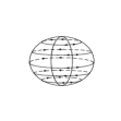
Figure 1. The phase portrait of system (3) for $a_{3}=a_{4}=a_{5}=a_{6}=a_{7}=a_{8}=0$.

Proposition 16.

The origin of (15) cannot be a nilpotent center, i.e. if tr$(D\widetilde{X}(0,0))=\det(D\widetilde{X}(0,0))=0$ and $|a_{4}|+|a_{5}|+|a_{7}|+|a_{8}|\neq 0$, then $(0,0)$ is not a center.

Proof.

As tr$(D\widetilde{X}(0,0))=\det(D\widetilde{X}(0,0))=0$, i.e. $a_{8}=-a_{4}$ and $a_{4}^{2}+a_{7}a_{5}=0$, we suppose first that $a_{4}a_{7}\neq 0$. Therefore, $a_{5}=\displaystyle-a_{4}^{2}/a_{7}$. Doing the change of variables $u=r-\displaystyle s/a_{4}$, $v=\displaystyle a_{7}s/a_{4}$ system (15) can be written as

(16) $$\dot{r}=s+P_{2}(r,s),\;\;\dot{s}=Q_{2}(r,s).$$

Let $\varphi(r)=\alpha_{1}r+\alpha_{2}r^{2}+\cdots$ the solution of $s+P_{2}(r,s)=0$. Therefore, $\alpha_{1}=0$ and $\alpha_{2}=\displaystyle(a_{1}a_{4}+a_{2}a_{7})/a_{7}$. If $\alpha_{2}=0$, then in the above system $(0,0)$ cannot be a center because in this case it is not an isolated singularity. Now, if $\alpha_{2}\neq 0$, substituting $\varphi$ in $\psi(r)=Q_{2}(r,\varphi(r))$ we obtain that $\psi(r)=\beta_{2}r^{2}+\cdots$, where $\beta_{2}=\displaystyle((a_{4}^{2}+a_{7}^{2})(a_{4}a_{1}+a_{7}a_{2}))/(a_{4}a_{7})$. Hence, as $\beta_{2}\neq 0$, it follows, by Theorem $67$ of page $362$ of [1], that $(0,0)$ is not a center.

Now, we have to study the case $a_{4}^{2}+a_{5}a_{7}=0$, $a_{4}a_{7}=0$ and $|a_{4}|+|a_{5}|+|a_{7}|\neq 0$. Therefore, we have two possibilities $a_{4}=a_{5}=0$, $a_{7}\neq 0$ and $a_{4}=a_{7}=0$, $a_{5}\neq 0$ for system (15). But, as these two possibilities are equivalent by the change of variables $(u,v)\mapsto(v,u)$, we need to study only the last one. Therefore, after a rescaling of time given by $d\tau=-a_{5}dt$ in (15), we obtain a system of the form

(17) $$\dot{u}=s+P_{2}(u,v),\;\;\dot{v}=Q_{2}(u,v).$$

Note that $a_{1}\neq 0$ in (17), otherwise $(0,0)$ is not an isolated singularity. As in the previous case, we have that $\varphi(u)\equiv 0$ is the solution of $v+P_{2}(u,v)=0$ and $\psi(u)=Q_{2}(u,\varphi(u))=\displaystyle(a_{1}u^{2})/a_{5}+\cdots$. Hence, by the same argument $(0,0)$ is not a center. ∎

Before proving Theorem 2 we do one remak.

Remark 17.

Let $U$ be an open subset of $\mathbb{R}^{2}$, $F:U\rightarrow\mathbb{R}$ be an analytic function which is not identically zero on $U$ and $X$ be a polynomial vector field associated to a system of the form

(18) $$\dot{x}=P(x,y),\;\;\;\dot{y}=Q(x,y),$$

where $P$ and $Q$ are polynomials in the variables $x$ and $y$ with real coefficients. The function $F$ is an integrating factor of this polynomial system on $U$ if one of the following three equivalent conditions holds on $U$ $\displaystyle\frac{\partial(FP)}{\partial x}=-\frac{\partial(FQ)}{\partial x}$, ${\rm div}(FP,FQ)=0$, $XF=-F\;{\rm div}(P,Q)$. As usual the divergence of the vector field $X$ is defined by ${\rm div}(X)={\rm div}(P,Q)=\displaystyle\frac{\partial P}{\partial x}+\frac{\partial Q}{\partial y}$.

The first integral $H$ associated to the integrating factor $F$ is given by

(19) $$H(x,y)=\int F(x,y)P(x,y)dy+h(x),$$

where $h(x)$ is chosen in order that it satisfies $\displaystyle\frac{\partial H}{\partial x}=-FQ$. Note that $\displaystyle\frac{\partial H}{\partial y}=FP$, so that $XH\equiv 0$. The function $H$ is single–valued, if $U$ is simply connected and $F\not\equiv 0$.

Conversely, given a first integral $H$ of the system associated to $X$ we always can find an integrating factor $F$ such that $\displaystyle\frac{\partial H}{\partial y}=FP$ and $\displaystyle\frac{\partial H}{\partial x}=-FQ$.

Let $V:U\rightarrow\mathbb{R}$ be an analytic function which is not identically zero on $U$. The function $V$ is an inverse integrating factor of the polynomial system (18) on $U$ if

(20) $$P\frac{\partial V}{\partial x}+Q\frac{\partial V}{\partial y}=\left(\frac{\partial P}{\partial x}+\frac{\partial Q}{\partial y}\right)V.$$

We note that $\{V=0\}$ is formed by orbits of system (18) and $F=1/V$ defines on $U\setminus\{V=0\}$ an integrating factor of (18).

Proof of Theorem 2. We have that if tr$(D\widetilde{X}(0,0))=0$ and $\det(D\widetilde{X}(0,0))>0$, i.e. $a_{8}=-a_{4}$ and $a_{4}^{2}+a_{7}a_{5}<0$, then the origin can be a linear type center or a weak focus. Note that in this case $a_{5}a_{7}\neq 0$. Hence, doing the change of variables $u=-\displaystyle\sqrt{-(a_{4}^{2}+a_{7}a_{5})}r/a_{7}+a_{4}s/a_{7}$, $v=s$ and introducing the new time variable $\tau$ through $d\tau=\sqrt{-(a_{4}^{2}+a_{7}a_{5})}\,\,dt$ system (15) can be written as

(21) $$\dot{r}=-s+P_{2}(r,s)+P_{3}(r,s),\;\;\dot{s}=r+Q_{2}(r,s)+Q_{3}(r,s),$$

where $P_{2}$, $P_{3}$, $Q_{2}$ and $Q_{3}$ are respectively the homogeneous parts of degree $2$ and $3$ of the above system. We have that the origin of this system is a center if and only if its Lyapunov coefficients $V_{i}$ are zero. Therefore, we have to determine the Lyapunov coefficients $V_{i}$ that can be obtained from

(22) $$P\frac{\partial H}{\partial r}+Q\frac{\partial H}{\partial s}=\sum_{i=1}^{\infty}V_{i}(r^{2}+s^{2})^{i+1},$$

where $H(r,s)=\displaystyle 1/2(r^{2}+s^{2})+\sum^{\infty}_{j=3}H_{j}(r,s)$ and $H_{j}$ are homogeneous polynomial of degree $j$.

We will show that if $V_{1}=0$, then $V_{k}=0$ for all $k\in\mathbb{N}$. From the homogeneous part of degree two, three and four of (22), we obtain the following system

(23) $$\begin{array}[]{rcl}\displaystyle-s\frac{\partial H_{2}}{\partial r}+r\frac{\partial H_{2}}{\partial s}&\equiv&0,\\ \displaystyle-s\frac{\partial H_{3}}{\partial r}+r\frac{\partial H_{3}}{\partial s}+P_{2}\frac{\partial H_{2}}{\partial r}+Q_{2}\frac{\partial H_{2}}{\partial s}&=&0,\\ \displaystyle-s\frac{\partial H_{4}}{\partial r}+r\frac{\partial H_{4}}{\partial s}+P_{2}\frac{\partial H_{3}}{\partial r}+Q_{2}\frac{\partial H_{3}}{\partial s}+P_{3}\frac{\partial H_{2}}{\partial r}+Q_{3}\frac{\partial H_{2}}{\partial s}&=&V_{1}(r^{2}+s^{2})^{2}.\end{array}$$

Solving system (23), we obtain that $V_{1}=((a_{5}-a_{7})(a_{4}(a_{1}^{2}-a_{2}^{2})+a_{1}a_{2}(a_{5}+a_{7})))/(8a_{7}(-a_{4}^{2}-a_{5}a_{7})^{3/2})$. Now, as $a_{4}^{2}+a_{5}a_{7}<0$, we have that $a_{5}\neq a_{7}$. Therefore, $V_{1}=0$ if and only if $a_{4}(a_{1}^{2}-a_{2}^{2})+a_{1}a_{2}(a_{5}+a_{7})=0$. Hence, we distinguish the following four cases.

Case 1: $a_{1}=a_{4}=0$ and $a_{2}\neq 0$. In this case system (15) becomes

(24) $$\dot{u}=-a_{5}v+a_{2}v^{2}-(a_{5}+a_{7})u^{2}v,\;\;\dot{v}=-a_{7}u-a_{2}uv-(a_{5}+a_{7})uv^{2}.$$

This system is invariant with respect to the change of variables $(u,v,t)\mapsto(-u,v,-t)$, i.e. it is symmetric with respect to the straight line $u=0$. Therefore, in this case $(0,0)$ is a center.

Case 2: $a_{2}=0$ and $a_{1}\neq 0$. Then $a_{4}=0$. In this case system (15) becomes

(25) $$\dot{u}=-a_{5}v+a_{1}uv-(a_{5}+a_{7})u^{2}v,\;\;\dot{v}=-a_{7}u-a_{1}u^{2}-(a_{5}+a_{7})uv^{2}.$$

We have that system $(\ref{eq:124})$ becomes $(\ref{eq:123})$ by the change of variables $(u,v)\mapsto(v,u)$. Therefore, this case is equivalent to Case $1$.

Case 3: $a_{1}=a_{2}=0$. In this case system (15) becomes

(26) $$\begin{array}[]{lcl}\dot{u}&=&-a_{4}u-a_{5}v-a_{4}u^{3}-(a_{5}+a_{7})u^{2}v+a_{4}uv^{2},\\ \dot{v}&=&-a_{7}u+a_{4}v-a_{4}u^{2}v-(a_{5}+a_{7})uv^{2}+a_{4}v^{3}.\end{array}$$

This system has a first integral given by $H(u,v)=((a_{7}+a_{5})u^{2}-2a_{4}uv+a_{5})/((a_{5}-a_{7})u^{2}+2a_{4}uv+2a_{5}v^{2}+a_{5})$. As $H$ is defined in $(0,0)$, it follows that in this case $(0,0)$ is a center.

Case 4: $a_{1}a_{2}\neq 0$. In this case $V_{1}=0$ implies that $a_{5}=\displaystyle(a_{4}(a_{2}^{2}-a_{1}^{2})-a_{1}a_{2}a_{7})/(a_{1}a_{2})$. Note that $-(a_{4}^{2}+a_{5}a_{7})>0$ becomes $\displaystyle((a_{1}a_{4}+a_{2}a_{7})(a_{1}a_{7}-a_{2}a_{4}))/(a_{1}a_{2})>0$. Now, this case is equivalent to Case $1$ doing the orthogonal linear change of variables

$$\left(\begin{array}[]{c}x\\ y\\ z\end{array}\right)=\left(\begin{array}[]{ccc}\displaystyle-\frac{a_{2}}{\sqrt{a_{1}^{2}+a_{2}^{2}}}&\displaystyle\frac{a_{1}}{\sqrt{a_{1}^{2}+a_{2}^{2}}}&0\\ \displaystyle\frac{a_{1}}{\sqrt{a_{1}^{2}+a_{2}^{2}}}&\displaystyle\frac{a_{2}}{\sqrt{a_{1}^{2}+a_{2}^{2}}}&0\\ 0&0&1\end{array}\right)\left(\begin{array}[]{c}\tilde{x}\\ \tilde{y}\\ \tilde{z}\end{array}\right),$$

where the $a_{i}$’s denote the coefficients of $X$ in the variables $(x,y,z)$ satisfying the hypothesis. In fact, denoting by $\tilde{a}_{i}$ the coefficients of system (3) in the variables $(\tilde{x},\tilde{y},\tilde{z})$, we have that $\tilde{a}_{1}=\tilde{a}_{3}=\tilde{a}_{4}=\tilde{a}_{6}=\tilde{a}_{8}=0$, $\tilde{a}_{2}=-\sqrt{a_{2}^{2}+a_{1}^{2}}$, $\tilde{a}_{5}=(a_{1}a_{7}-a_{2}a_{4})/a_{1}$, $\tilde{a}_{7}=-(a_{1}a_{4}+a_{2}a_{7})/a_{2}$. Note that $\tilde{a}_{2}\neq 0$ and $\tilde{a}_{5}\tilde{a}_{7}<0$. This completes the proof of the theorem. $\Box$

5. Two criteria for determining the nonexistence of limit cycles for homogeneous polynomial vector fields on $\mathbb{S}^{2}$

Let $X=(P,Q,R)$ be a homogeneous polynomial vector field on $\mathbb{S}^{2}$ of degree $m$. The next proposition will be necessary for proving the results of this section, see its proof in [11].

Proposition 18.

Let $f(x,y,z)=x^{2}+y^{2}+z^{2}-1$ and let $X$ be a homogeneous polynomial vector field on $\mathbb{S}^{2}$. Then $f$ is a first integral of $X$ in $\mathbb{R}^{3}$, i. e. $P(x,y,z)x+Q(x,y,z)y+R(x,y,z)z=0$ for all $(x,y,z)\in\mathbb{R}^{3}$.

Let $(a,b,c)\in\mathbb{S}^{2}$, we can suppose that $X$ does not have a limit cycle such that $(a,b,c)$ belongs it, because we can do a rotation of $SO(3)$ which preserves all properties of $X$. Hence, the study of the existence of limit cycles of $X$ on $\mathbb{S}^{2}$ is equivalent to study the existence of limit cycles of the planar vector field induced by $X$ through the stereographic projection (10) at the point $(a,b,c)$. We will consider the cases when $(a,b,c)$ is the point $(0,0,1)$, i.e. the planar vector field determined by system (14). We denote this planar vector field by

$$\bar{X}=(\bar{P},\bar{Q})=(\tilde{P}+u\tilde{R},\tilde{Q}+v\tilde{R}).$$

Here $\tilde{F}(u,v)=F(2u,2v,u^{2}+v^{2}-1)$ with $F\in\mathbb{R}[x,y,z]$.

Now we state a result that can be found in [8] and that will be necessary for the proof of Theorem 3.

Theorem 19.

Let $(\mathcal{P},\mathcal{Q})$ be a $C^{1}$ vector field defined in an open subset $U$ of  $\mathbb{R}^{2}$, $(\alpha(t),\beta(t))$ a periodic solution of $(\mathcal{P},\mathcal{Q})$ of period $\tau$, $K:U\longrightarrow\mathbb{R}$ a $C^{1}$ map such that $\int^{\tau}_{0}K(\alpha(t),\beta(t))dt\neq 0$, and $f=f(x,y)$ a $C^{1}$ solution of the linear partial differential equation $\displaystyle\mathcal{P}\frac{\partial f}{\partial x}+\mathcal{Q}\frac{\partial f}{\partial y}=Kf$. Then the closed trajectory $\gamma=\{(\alpha(t),\beta(t))\in U:\;t\in[0,\tau]\}$ is contained in $\Sigma=\{(x,y)\in U:\;f(x,y)=0\}$, and $\gamma$ is not contained in a period annulus of $(\mathcal{P},\mathcal{Q})$. Moreover, if the vector field $(\mathcal{P},\mathcal{Q})$ is analytic, then $\gamma$ is a limit cycle.

Proof of Theorem 3. Consider the function $f(u,v)=u^{2}+v^{2}+1$. Using the previous notation we have that

$$\bar{P}\frac{\partial f}{\partial u}+\bar{Q}\frac{\partial f}{\partial v}=2u\tilde{P}+2u^{2}\tilde{R}+2v\tilde{Q}+2v^{2}\tilde{R}=2u\tilde{P}+2v\tilde{Q}+2(u^{2}+v^{2})\tilde{R}.$$

Note that, by Proposition 18, $2u\tilde{P}+2v\tilde{Q}+(u^{2}+v^{2}-1)\tilde{R}=0$. Therefore,

$$\bar{P}\frac{\partial f}{\partial u}+\bar{Q}\frac{\partial f}{\partial v}=-(u^{2}+v^{2}-1)\tilde{R}+2(u^{2}+v^{2})\tilde{R}=\tilde{R}(u^{2}+v^{2}+1)=\tilde{R}f.$$

Therefore, $f=0$ is an invariant algebraic curve of $\bar{X}$ and $\tilde{R}$ is its cofactor.

Using the notation of Theorem 19 we assume that $\gamma$ is a periodic orbit of $\bar{X}$. Now, if $\tilde{R}$ does not change sign in $\mathbb{R}^{2}$, then $\int_{\gamma}\tilde{R}dt\neq 0$, and since $\{(u,v)\in\mathbb{R}^{2}:\;f(u,v)=0\}=\emptyset$, by Theorem 19 $\bar{X}$ does not have periodic orbits. Hence, $X$ does not have periodic orbits on $\mathbb{S}^{2}$. This proves statement (a).

Now we will prove statement (b). Note that

$$\langle\bar{X},\nabla\tilde{R}\rangle\mid_{\tilde{R}=0}=\left(\tilde{P}\frac{\partial\tilde{R}}{\partial u}+\tilde{Q}\frac{\partial\tilde{R}}{\partial v}\right)\mid_{\tilde{R}=0}=\langle(\tilde{P},\tilde{Q}),\nabla\tilde{R}\rangle\mid_{\tilde{R}=0}.$$

Therefore, if $\langle(\tilde{P},\tilde{Q}),\nabla\tilde{R}\rangle\mid_{\tilde{R}=0}$ does not change sign, then the vector field $\bar{X}$ is transversal to the curve $\tilde{R}=0$, so there are no periodic orbits of $\bar{X}$ intersecting the curve $\tilde{R}=0$. Hence, if $X$ has a periodic orbit $\gamma$, then $\gamma\subset\mathbb{R}^{2}\setminus\{\tilde{R}=0\}$. Thus, $\int_{\gamma}\tilde{R}dt\neq 0$, and so by Theorem 19 we get $\gamma\subset\{(u,v)\in\mathbb{R}^{2}:\;f(u,v)=0\}=\emptyset$. Therefore, $\bar{X}$ does not have periodic orbits, i.e. $X$ does not have periodic orbits on $\mathbb{S}^{2}$. $\Box$

From the proof of Theorem 3 we have:

Corollary 20.

The vector field $\bar{X}$ has the invariant algebraic curve $f(u,v)=u^{2}+v^{2}+1=0$ with cofactor $K_{f}=\tilde{R}$.

We see in the beginning of this section that the study of the existence of limit cycles of homogeneous vector fields $X$ on $\mathbb{S}^{2}$ is equivalent to study the existence of limit cycles of the planar vector fields induced by $X$ through the stereographic projection at the point $(a,b,c)$. But sometimes it is necessary to do a rotation in order that $(a,b,c)$ does not belong to a limit cycle of $X$. In fact, if $(a,b,c)$ belongs to the limit cycle $\gamma$ then, as the phase portrait of $X$ is symmetric with respect to the origin, we have that $-(a,b,c)\in-\gamma=\{-(x,y,z):\;(x,y,z)\in\gamma\}$. If degree of $X$ is even, by Proposition $4$ of [12], $\gamma\neq-\gamma$. Therefore, if the degree of $X$ is even, it is not necessary to do a rotation. Now if degree of $X$ is odd, by Proposition $6$ of [12] we know that the case $\gamma=-\gamma$ is possible.

Now, we will consider the the planar vector fields $\bar{X}_{i}$, $i=1,2,3$, determined by systems (5), (6) and (42), i.e.

$$\begin{array}[]{lcl}\bar{X}_{1}&=&(\bar{P}_{1},\bar{Q}_{1})=(\tilde{P}_{1}-(u+a)\tilde{\mathcal{K}}_{1},\tilde{Q}_{1}-(v+b)\tilde{\mathcal{K}}_{1}),\\ \bar{X}_{2}&=&(\bar{P}_{2},\bar{Q}_{2})=(\tilde{Q}_{2}-(u+b)\tilde{\mathcal{K}}_{2},\tilde{R}_{2}-(v+c)\tilde{\mathcal{K}}_{2}),\\ \bar{X}_{3}&=&(\bar{P}_{3},\bar{Q}_{3})=(\tilde{P}_{3}-(u+a)\tilde{\mathcal{K}}_{3},\tilde{R}_{3}-(v+c)\tilde{\mathcal{K}}_{3}).\end{array}$$

Here $\mathcal{K}=aP+bQ+cR$, $\tilde{F}_{1}(u,v)=F(u+a,v+b,c-(au+bv)/c)$, $\tilde{F}_{2}(u,v)=F(a-(bu+cv)/a,u+b,v+c)$ and $\tilde{F}_{3}(u,v)=F(u+a,b-(au+cv)/b,v+c)$ and $F\in\mathbb{R}[x,y,z]$.

Proof of Theorem 4. First we will prove statement $(a)$. Consider the function

$$\begin{array}[]{lcl}f_{1}(u,v)&=&\displaystyle(u+a)^{2}+(v+b)^{2}+\left(c-\frac{au+bv}{c}\right)^{2}\\ &=&\displaystyle\frac{a^{2}+c^{2}}{c^{2}}u^{2}+\frac{2ab}{c^{2}}uv+\frac{b^{2}+c^{2}}{c^{2}}v^{2}+1.\end{array}$$

Using the previous notation we have that

$$\begin{array}[]{lcl}\displaystyle\bar{P}_{1}\frac{\partial f_{1}}{\partial u}+\bar{Q}_{1}\frac{\partial f_{1}}{\partial v}&=&\displaystyle\tilde{P}_{1}\frac{\partial f_{1}}{\partial u}+\tilde{Q}_{1}\frac{\partial f_{1}}{\partial v}-2\tilde{\mathcal{K}}_{1}(f_{1}-1)-\frac{2}{c^{2}}\tilde{\mathcal{K}}_{1}(au+bv)\\ &=&\displaystyle-2\tilde{\mathcal{K}}_{1}(f_{1}-1)+\frac{2}{c^{2}}(c^{2}u\tilde{P}_{1}+c^{2}v\tilde{Q}_{1}-c(au+bv)\tilde{R}_{1}).\end{array}$$

Note that, by Proposition 18, $(u+a)\tilde{P}_{1}+(v+b)\tilde{Q}_{1}+(c-(au+bv)/c)\tilde{R}_{1}=0$, i.e. $c^{2}u\tilde{P}_{1}+c^{2}v\tilde{Q}_{1}-c(au+bv)\tilde{R}_{1}=-c^{2}\tilde{\mathcal{K}}_{1}$. Therefore, $\displaystyle\bar{P}_{1}\frac{\partial f_{1}}{\partial u}+\bar{Q}_{1}\frac{\partial f_{1}}{\partial v}=-2\tilde{\mathcal{K}}_{1}(f_{1}-1)-2\tilde{\mathcal{K}}_{1}=-2\tilde{\mathcal{K}}_{1}f_{1}$. Hence, $f_{1}=0$ is an invariant algebraic curve of $\bar{X}_{1}$ and $-2\tilde{\mathcal{K}}_{1}$ is its cofactor.

Using the notation of Theorem 19 we assume that $\gamma$ is a periodic orbit of $\bar{X}_{1}$. Now, if $\tilde{\mathcal{K}}_{1}$ does not change sign in $\mathbb{R}^{2}$, then $\int_{\gamma}\tilde{\mathcal{K}}_{1}dt\neq 0$, and since $\{(u,v)\in\mathbb{R}^{2}:\;f_{1}(u,v)=0\}=\emptyset$, by Theorem 19 $\bar{X}_{1}$ does not have periodic orbits. Hence, $X$ does not have periodic orbits on $\mathbb{S}^{2}$. This proves statement (a).

Now we will prove statement (b). Note that

$$\langle\bar{X}_{1},\nabla\tilde{\mathcal{K}}_{1}\rangle\mid_{\tilde{\mathcal{K}}_{1}=0}=\left(\tilde{P}_{1}\frac{\partial\tilde{\mathcal{K}}_{1}}{\partial u}+\tilde{Q}_{1}\frac{\partial\tilde{\mathcal{K}}_{1}}{\partial v}\right)\mid_{\tilde{\mathcal{K}}_{1}=0}=\langle(\tilde{P}_{1},\tilde{Q}_{1}),\nabla\tilde{\mathcal{K}}_{1}\rangle\mid_{\tilde{\mathcal{K}}_{1}=0}.$$

Therefore, if $\langle(\tilde{P}_{1},\tilde{Q}_{1}),\nabla\tilde{\mathcal{K}}_{1}\rangle\mid_{\tilde{\mathcal{K}}_{1}=0}$ does not change sign, then the vector field $\bar{X}_{1}$ is transversal to the curve $\tilde{\mathcal{K}}_{1}=0$, so there are no periodic orbits of $\bar{X}_{1}$ intersecting the curve $\tilde{\mathcal{K}}_{1}=0$. Hence, if $X$ has a periodic orbit $\gamma$, then $\gamma\subset\mathbb{R}^{2}\setminus\{\tilde{\mathcal{K}}_{1}=0\}$. Thus, $\int_{\gamma}\tilde{\mathcal{K}}_{1}dt\neq 0$, and so by Theorem 19 we get $\gamma\subset\{(u,v)\in\mathbb{R}^{2}:\;f_{1}(u,v)=0\}=\emptyset$. Therefore, $\bar{X}_{1}$ does not have periodic orbits, i.e. $X$ does not have periodic orbits on $\mathbb{S}^{2}$.

The proof of the other statements is similar replacing $f_{1}$ by

$$\begin{array}[]{lcl}f_{2}(u,v)&=&\displaystyle(u+b)^{2}+(v+c)^{2}+\left(a-\frac{bu+cv}{a}\right)^{2}\\ \end{array}$$

in the statements $(c)$, $(d)$ and by

$$\begin{array}[]{lcl}f_{3}(u,v)&=&\displaystyle(u+a)^{2}+(v+c)^{2}+\left(b-\frac{au+cv}{b}\right)^{2}\\ \end{array}$$

in the statements $(e)$, $(f)$. $\Box$

¿From the proof of Theorem 4, using the previous notation, we have the following corollaries:

Corollary 21.

The algebraic curve $f_{i}=0$ is an invariant algebraic curve of vector field $\bar{X}_{i}$ with cofactor $K_{f_{i}}=-2\tilde{\mathcal{K}}_{i}$, for $i=1,2,3$.

Corollary 22.

In the assumptions of Theorem 4, if $C$ is a periodic orbit, then $C$ is the unique periodic orbit of $X$ on $\mathbb{S}^{2}$.

We say that an orbit $\gamma$ of a homogeneous polynomial vector field on $\mathbb{S}^{2}$ is convex if for any $p\in\gamma$ the great circle tangent to $\gamma$ at $p$ intersects $\gamma$ only at $p$, or $\gamma$ is entirely contained in the great circle.

Proposition 23.

Let $X=(P,Q,R)$ be a quadratic homogeneous polynomial vector field on $\mathbb{S}^{2}$. Any great circle in $\mathbb{S}^{2}$ has at most four tangencies with the orbits of $X$ or is formed by orbits of $X$.

Proposition 24.

Let $X$ be a homogeneous polynomial vector field on $\mathbb{S}^{2}$ of degree $2$. Any periodic orbit of $X$ on $\mathbb{S}^{2}$ is convex.

Propositions 23 and 24 also can be found in Camacho [2] or [17].

By Proposition 24 we have that in the case that $X$ has degree $2$ the hypotheses of Theorem 4 is not necessary, i.e. we can suppose that all periodic orbits of $X$ are contained on the hemisphere determined by the plane $ax+by+cz=0$ such that $(a,b,c)$ belongs it.

6. Phase portraits for homogeneous polynomial vector fields on $\mathbb{S}^{2}$ of degree $2$ having some non–hyperbolic singularity

Let $p$ be a singularity of a homogeneous polynomial vector field $X$ on $\mathbb{S}^{2}$ of degree $2$. By Proposition 14, we can suppose without loss of generality that $p=(0,0,-1)$, then the classification of singularities of $X$ is equivalent to the classification of singularities of (15) at the origin.

Using the notation of the previous section we say that $p$ is a hyperbolic singularity of $X$ if the eigenvalues of $D\widetilde{X}(0,0)$ have real part distinct of zero. We say that $p$ is a non–degenerate singularity if $\det(D\widetilde{X}(0,0))=a_{4}a_{8}-a_{5}a_{7}\neq 0$, a semi–hyperbolic singularity if tr$(D\widetilde{X}(0,0))=-a_{4}-a_{8}\neq 0$ and $\det(D\widetilde{X}(0,0))=0$, a nilpotent singularity if tr$(D\widetilde{X}(0,0))=\det(D\widetilde{X}(0,0))=0$ and $|a_{4}|+|a_{5}|+|a_{7}|+|a_{8}|\neq 0$, and linearly zero singularity if $D\widetilde{X}(0,0)$ is the null matrix.

The next result will be necessary for proving the results of this section and its proof can be found in [11].

Proposition 25.

Let $X$ be a homogeneous polynomial vector field of degree $2$ on $\mathbb{S}^{2}$. Suppose that $X$ has at least one invariant circle on $\mathbb{S}^{2}$, then $X$ has no limit cycles.

Proof of Theorem 5. Statement $(a)$ is exactly Proposition 15. Therefore, we have to prove only statements $(b)$, $(c)$ and $(d)$.

In what follows, by Proposition 14, we can suppose that the system associated to $X=(P,Q,R)$ is in the form (3) with $a_{3}=a_{6}=0$. Therefore, if $R\not\equiv 0$ then the equator of $\mathbb{S}^{2}$, i.e. $\mathbb{S}^{1}$ is not invariant by $X$, because $z$ is not a factor of $R$. Hence, in this case, on the Poincaré disc associated to $\tilde{X}$ we represent $\mathbb{S}^{1}$ by a circle formed by dots.

In the case that $X$ has a nilpotent singularity, to determine its phase portrait, from the proof of Proposition 16, it is sufficient to study the systems

(27) $$\begin{array}[]{lcl}\dot{x}&=&a_{1}xy+a_{2}y^{2}+a_{4}xz-\displaystyle\frac{a_{4}^{2}}{a_{7}}yz,\\ \dot{y}&=&=-a_{1}x^{2}-a_{2}xy+a_{7}xz-a_{4}yz,\\ \dot{z}&=&-a_{4}x^{2}+a_{4}y^{2}-\left(a_{7}-\displaystyle\frac{a_{4}^{2}}{a_{7}}\right)xy,\end{array}$$

with $a_{4}a_{7}\neq 0$, and

(28) $$\dot{x}=a_{1}xy+a_{2}y^{2}+a_{5}yz,\;\;\dot{y}=-a_{1}x^{2}-a_{2}xy,\;\;\dot{z}=-a_{5}xy,$$

with $a_{5}\neq 0$. Now system (27) is equivalent to system (28) by the orthogonal linear change of variables

$$\left(\begin{array}[]{c}x\\ y\\ z\end{array}\right)=\left(\begin{array}[]{ccc}\displaystyle\frac{a_{4}}{\sqrt{a_{4}^{2}+a_{7}^{2}}}&\displaystyle-\frac{a_{7}}{\sqrt{a_{4}^{2}+a_{7}^{2}}}&0\\ \displaystyle\frac{a_{7}}{\sqrt{a_{4}^{2}+a_{7}^{2}}}&\displaystyle\frac{a_{4}}{\sqrt{a_{4}^{2}+a_{7}^{2}}}&0\\ 0&0&1\end{array}\right)\left(\begin{array}[]{c}\tilde{x}\\ \tilde{y}\\ \tilde{z}\end{array}\right),$$

where $a_{i}$ are the coefficients of system (27). Denoting by $\tilde{a}_{i}$ the coefficients of system (27) in the variables $(\tilde{x},\tilde{y},\tilde{z})$, we have that $\tilde{a}_{1}=(a_{1}a_{4}+a_{2}a_{7})/\sqrt{a_{4}^{2}+a_{7}^{2}}$, $\tilde{a}_{2}=(a_{2}a_{4}-a_{1}a_{7})/\sqrt{a_{4}^{2}+a_{7}^{2}}$, $\tilde{a}_{5}=-(a_{4}^{2}+a_{7}^{2})/a_{7}$. Note that $\tilde{a}_{5}\neq 0$. Therefore, we have to study only system (28) or equivalently system (17) induced from it by the central projection. We distinguish two cases.

Case 1: $a_{1}\neq 0$. By the proof of Proposition 16 we have that $v=\varphi(u)\equiv 0$ is the solution of $v+P_{2}(u,v)=0$. Hence, $\psi(u)=Q_{2}(u,\varphi(u))=\displaystyle a_{1}u^{2}/a_{5}$ and $\displaystyle\frac{\partial P_{2}}{\partial u}(u,\varphi(u))+\displaystyle\frac{\partial Q_{2}}{\partial v}(u,\varphi(u))=\frac{a_{2}}{a_{5}}u$. Then, by Theorem $67$ of page $362$ of [1] it follows that $(0,0)$ is a cusp.

In the case $a_{2}\neq 0$ the vector field $X$ determined by system (28) does not have singularities on $\mathbb{S}^{1}$. Moreover, $X$ has four singularities $(0,0,\pm 1)$, $(0,a_{5}/(\sqrt{a_{2}^{2}+a_{5}^{2}}),\linebreak-a_{2}/(\sqrt{a_{2}^{2}+a_{5}^{2}}))$ and $(0,-a_{5}/(\sqrt{a_{2}^{2}+a_{5}^{2}}),a_{2}/(\sqrt{a_{2}^{2}+a_{5}^{2}}))$ corresponding to the singularities $(0,0)$ and $\left(0,a_{5}/a_{2}\right)$ of (17). We have that the eigenvalues associated to $\left(0,a_{5}/a_{2}\right)$ are $(-a_{1}\pm\sqrt{a_{1}^{2}-4(a_{2}^{2}+a_{5}^{2})})/2a_{2}$. Thus, $\left(0,a_{5}/a_{2}\right)$ can be a node or a focus of (17). Now, by the orthogonal linear change of variables

$$\left(\begin{array}[]{c}x\\ y\\ z\end{array}\right)=\left(\begin{array}[]{ccc}1&0&0\\ 0&\displaystyle\frac{a_{2}}{\sqrt{a_{2}^{2}+a_{5}^{2}}}&\displaystyle-\frac{a_{5}}{\sqrt{a_{2}^{2}+a_{5}^{2}}}\\ 0&\displaystyle\frac{a_{5}}{\sqrt{a_{2}^{2}+a_{5}^{2}}}&\displaystyle\frac{a_{2}}{\sqrt{a_{2}^{2}+a_{5}^{2}}}\end{array}\right)\left(\begin{array}[]{c}\tilde{x}\\ \tilde{y}\\ \tilde{z}\end{array}\right),$$

the system associated to $X$ becomes

(29) $$\begin{array}[]{lcl}\dot{\tilde{x}}&=&P(\tilde{x},\tilde{y},\tilde{z})=\displaystyle\frac{a_{1}a_{2}}{\sqrt{a_{2}^{2}+a_{5}^{2}}}\tilde{x}\tilde{y}-\frac{a_{1}a_{5}}{\sqrt{a_{2}^{2}+a_{5}^{2}}}\tilde{x}\tilde{z}+a_{2}\tilde{y}^{2}-a_{5}\tilde{y}\tilde{z},\\ \dot{\tilde{y}}&=&Q(\tilde{x},\tilde{y},\tilde{z})=-\displaystyle\frac{a_{1}a_{2}}{\sqrt{a_{2}^{2}+a_{5}^{2}}}\tilde{x}^{2}-a_{2}\tilde{x}\tilde{y}+a_{5}\tilde{x}\tilde{z},\\ \dot{\tilde{z}}&=&R(\tilde{x},\tilde{y},\tilde{z})=\displaystyle\frac{a_{1}a_{5}}{\sqrt{a_{2}^{2}+a_{5}^{2}}}\tilde{x}^{2}.\end{array}$$

Note that in these coordinates the singularity $(0,a_{5}/(\sqrt{a_{2}^{2}+a_{5}^{2}}),-a_{2}/(\sqrt{a_{2}^{2}+a_{5}^{2}}))$ correspond to the point $(0,0,-1)$. Hence, using the notation of Section 5, we have that $\tilde{R}(u,v)=R(2u,2v,u^{2}+v^{2}-1)=4a_{1}a_{5}/\sqrt{a_{2}^{2}+a_{5}^{2}}u^{2}$. Thus, $\tilde{R}$ does not change sign and by Theorem 3, $X$ does not have periodic orbits on $\mathbb{S}^{2}$. So the phase portrait of $\tilde{X}$ on the Poincaré disc is equivalent to one of Figure 2.

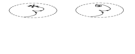
Figure 2. Phase portrait of Case $1$: $a_{1}a_{2}\neq 0$.

In the case $a_{2}=0$ the vector field $X$ has four singularities given by $(0,0,\pm 1)$ and $(0,\pm 1,0)$. The eigenvalues associated to the last two singularities are $\displaystyle 0,\;(a_{1}\pm\sqrt{a_{1}^{2}-4a_{5}^{2}})/2$ and $\displaystyle 0,\;-(a_{1}\pm\sqrt{a_{1}^{2}-4a_{5}^{2}})/2$, respectively. Therefore, these singularities can be nodes or foci. Now, substituting $a_{2}=0$ in the above change of coordinates we obtain that in this case the system associated to $X$ is equivalent to system (29) with $a_{2}=0$. Therefore, by the previous argument, we have that $X$ does not have limit cycles on $\mathbb{S}^{2}$. Thus, the phase portrait of $\tilde{X}$ on the Poincaré disc is equivalent to the one of Figure 3.

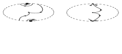
Figure 3. Phase portrait of Case $1$: $a_{1}\neq 0$ and $a_{2}=0$.

Case 2: $a_{1}=0$. In this case we have that (17) has the straight line of singularities $v=0$ and, so $X$ has an invariant circle formed by singularities determined by the intersection of the plane $y=0$ with $\mathbb{S}^{2}$. Moreover, $H(x,y,z)=\displaystyle a_{5}y-a_{2}z$ is a first integral of $X$ (note that $a_{5}\neq 0$) and $X$ has other two singularities $(0,a_{5},-a_{2})/(a_{2}^{2}+a_{5}^{2})$ and $(0,-a_{5},a_{2})/(a_{2}^{2}+a_{5}^{2})$. Then its phase portrait is equivalent to the one of Figure 4 $(a)$ if $a_{2}\neq 0$, or to the one Figure 4 $(b)$ if $a_{2}=0$. Hence, statement $(b)$ is proved.

\psfrag{A}[l][B]{$(a)$}\psfrag{B}[l][B]{$(b)$}\includegraphics[height=65.04256pt,width=144.54pt]{FigT21.eps}

Figure 4. Phase portrait of Case $2$.

Now, we prove statement $(c)$. By Theorem 2, we can suppose that $X$ is in the form (3) with $a_{3}=a_{6}=0$, $a_{8}=-a_{4}$, $a_{4}^{2}+a_{7}a_{5}<0$ and $a_{4}(a_{1}^{2}-a_{2}^{2})+a_{1}a_{2}(a_{5}+a_{7})=0$. Moreover, by the proof of Theorem 2, for characterizing the phase portrait of $X$ we have to study only systems (24) and (26). Therefore, we distinguish the following two cases.

Case 3: $a_{1}=0$ and $a_{2}\neq 0$. Then $a_{4}=0$. This case correspond to system (24). First we suppose that $a_{7}\neq-a_{5}$. In this case $X$ has only two singularities on $\mathbb{S}^{1}$, given by $(\pm 1,0,0)$ having eigenvalues $\{0,-(a_{2}\pm\sqrt{a_{2}^{2}-4(a_{7}^{2}+a_{5}a_{7})})/2\}$ and $\{0,(a_{2}\pm\sqrt{a_{2}^{2}-4(a_{7}^{2}+a_{5}a_{7})})/2\}$, respectively. The system induced by $X$ through the central projection, i.e. system (24) has a center in $(0,0)$ and another singularity $\left(0,a_{5}/a_{2}\right)$ with eigenvalues $\pm\sqrt{-(a_{2}^{2}+a_{5}^{2})(a_{5}^{2}+a_{5}a_{7})}/a_{2}$. Note that

(30) $$(a_{5}^{2}+a_{5}a_{7})(a_{7}^{2}+a_{5}a_{7})=(a_{5}+a_{7})^{2}a_{5}a_{7}<0,$$

because $a_{5}a_{7}<0$ and $a_{5}+a_{7}\neq 0$. Therefore, if the singularities on $\mathbb{S}^{1}$ are saddles, then $\left(0,\displaystyle a_{5}/a_{2}\right)$ is a center because system $(\ref{eq:123})$ is invariant with respect to the change of variables $(u,v,t)\mapsto(-u,v,-t)$. Now if $\left(0,\displaystyle a_{5}/a_{2}\right)$ is a saddle, then the singularities of $X$ on $\mathbb{S}^{1}$ can be nodes or foci. Note that if $a_{2}^{2}-4(a_{7}^{2}+a_{5}a_{7})\geq 0$ then $\{f_{\pm}=0\}\cap\mathbb{S}^{2}$, where $f_{\pm}(x,y,z)=y+2a_{7}z/(-a_{2}\pm\sqrt{a_{2}^{2}-4(a_{7}^{2}+a_{5}a_{7})})$, are invariant circles of $X$ on $\mathbb{S}^{2}$ with cofactors $K_{\pm}(x,y,z)=(-a_{2}\pm\sqrt{a_{2}^{2}-4(a_{7}^{2}+a_{5}a_{7})})x/2$. Therefore, in the case that the singularities of $X$ on $\mathbb{S}^{1}$ are either saddles or nodes, then $X$ has at least an invariant circle on $\mathbb{S}^{2}$. Hence, by Corollary 25 $X$ has no limit cycles on $\mathbb{S}^{2}$. Thus, in this case, the phase portrait of $X$ on the Poincaré disc is equivalent to the one of Figures 5 $(a)$ or $(b)$ on $\mathbb{S}^{2}$.

Now, we consider the planar vector field induced by $X$ through the stereographic projection (10) at the point (0,0,1), i.e. we consider system (14) which in this case becomes

(31) $$\begin{array}[]{lcl}\dot{u}&=&-2a_{5}v+4a_{2}v^{2}-2(a_{5}+2a_{7})u^{2}v+2a_{5}v^{3},\\ \dot{v}&=&-2a_{7}u-4a_{2}uv-2(a_{7}+2a_{5})uv^{2}+2a_{7}u^{3}.\end{array}$$

This system has an inverse integrating factor (see Remark 17) given by $V(u,v)=(u^{2}+v^{2}+1)V_{2}(u,v)$, where $V_{2}(u,v)=a_{7}u^{4}+2(a_{7}(v^{2}-1)-a_{2}v)u^{2}+a_{7}(1+v^{2})^{2}+2v(2a_{5}v+a_{2}(1-v^{2}))$. Note that que the roots of $V_{2}=0$ in $u$ are

$$u=\pm\frac{\sqrt{a_{7}(a_{7}v^{2}+a_{2}v+a_{7}\pm|v|\sqrt{a_{2}^{2}-4(a_{7}^{2}+a_{5}a_{7})})}}{a_{7}}.$$

Therefore, if $a_{2}^{2}-4(a_{7}^{2}+a_{5}a_{7})<0$, $V_{2}$ vanish only on the points $(\pm 1,0)$. Hence, by Remark 17, system (31) has a first integral defined on $\mathbb{R}^{2}\setminus\{(\pm 1,0)\}$. Hence, system (31) does not have limit cycles. Therefore, if the singularities of $X$ on $\mathbb{S}^{1}$ are foci, then the phase portrait of $X$ on the Poincaré disc is equivalent to Figure 5 $(c)$.

\psfrag{A}[l][B]{$(a)$}\psfrag{B}[l][B]{$(b)$}\psfrag{C}[l][B]{$(c)$}\includegraphics[height=72.26999pt,width=202.35622pt]{FigT22.eps}

Figure 5. Phase portrait of Case $3$: $a_{1}=a_{4}=0$, $a_{2}\neq 0$ and $a_{7}\neq-a_{5}$.

Now if $a_{7}=-a_{5}$, then the system associated to $X$ becomes

$$\dot{x}=y(a_{2}y+a_{5}z),\;\;\dot{y}=-x(a_{2}y+a_{5}z),\;\;\dot{z}=0.$$

Therefore, the phase portrait of $X$ on $\mathbb{S}^{2}$ in this case is equivalent to Figure 4 $(a)$.

Case 4: $a_{1}=a_{2}=0$. This case correspond to system $(\ref{eq:125})$. We claim that we can reduce to the case $a_{4}=0$. Now we prove the claim. In fact, consider the system associated to $X$ on $\mathbb{S}^{2}$, i.e. system (3) with $a_{1}=a_{2}=a_{3}=a_{6}=0$, $a_{8}=-a_{4}$ and $a_{4}^{2}+a_{7}a_{5}<0$. If $a_{4}\neq 0$ and $a_{5}+a_{7}\neq 0$, by the orthogonal linear change of variables

$$\left(\begin{array}[]{c}x\\ y\\ z\end{array}\right)=\left(\begin{array}[]{ccc}a&b&0\\ d&e&0\\ 0&0&1\end{array}\right)\left(\begin{array}[]{c}\tilde{x}\\ \tilde{y}\\ \tilde{z}\end{array}\right),$$

where $a=a_{4}\sqrt{2\sigma}/((a_{5}+a_{7})\sqrt{\delta\beta})$, $b=(a_{5}(a_{5}+a_{7})\delta-(2a_{4}^{2}+a_{5}(a_{5}+a_{7}))\sqrt{\sigma})/\sqrt{\delta\beta\gamma}$, $d=-\sqrt{\beta}/\sqrt{2\delta}$, $e=-(a_{4}((a_{5}+a_{7})(4a_{4}^{2}+a_{7}(a_{5}+a_{7})+a_{5}(a_{5}+a_{7}))+(a_{7}-a_{5})\sqrt{\sigma}))\sqrt{\delta\beta\gamma}$, $\delta=(a_{5}+a_{7})^{2}+4a_{4}^{2}$, $\sigma=(a_{5}+a_{7})^{2}\delta,\;\beta=\delta-\sqrt{\sigma}$, $\gamma=(a_{5}+a_{7})^{2}(a_{5}^{2}+a_{7}^{2}+2a_{4}^{2})+(a_{7}^{2}-a_{5}^{2})\sqrt{\sigma}$, we obtain $\tilde{a}_{4}=0$. Here $\tilde{a}_{i}$ denote the coefficients of system associated to $X$ on the variables $(\tilde{x},\tilde{y},\tilde{z})$. Note that in this case $\delta>0$, $\sigma>0$ and as $(\delta-\sqrt{\sigma})(\delta+\sqrt{\sigma})=4a_{4}^{2}\delta$, $((a_{5}+a_{7})^{2}(a_{5}^{2}+a_{7}^{2}+2a_{4}^{2})+(a_{7}^{2}-a_{5}^{2})\sqrt{\sigma})\cdot((a_{5}+a_{7})^{2}(a_{5}^{2}+a_{7}^{2}+2a_{4}^{2})-(a_{7}^{2}-a_{5}^{2})\sqrt{\sigma})=4(a_{5}+a_{7})^{4}(a_{4}^{2}+a_{5}a_{7})^{2}$, it follows that $\beta>0$, $\gamma>0$. Moreover, we have that $\tilde{a}_{1}=\tilde{a}_{2}=\tilde{a}_{3}=\tilde{a}_{4}=\tilde{a}_{6}=\tilde{a}_{8}=0$, $\tilde{a}_{5}=-\sqrt{2}(a_{5}+a_{7})(a_{5}a_{7}+a_{4}^{2})/\sqrt{\gamma}$ and $\tilde{a}_{7}=-\sqrt{\gamma}/(\sqrt{2}(a_{5}+a_{7}))$. Note that $\tilde{a}_{5}\tilde{a}_{7}<0$.

Now, if $a_{4}\neq 0$ and $a_{7}=-a_{5}$, then $a_{4}^{2}-a_{5}^{2}<0$ and doing the orthogonal linear change of variables

$$\left(\begin{array}[]{c}x\\ y\\ z\end{array}\right)=\left(\begin{array}[]{ccc}\displaystyle\frac{\sqrt{2a_{4}^{2}}}{2a_{4}}&\displaystyle\frac{a_{4}+a_{5}}{\sqrt{2(a_{5}+a_{4})^{2}}}&0\\ \displaystyle\frac{\sqrt{2a_{4}^{2}}}{2a_{4}}&\displaystyle-\frac{a_{4}+a_{5}}{\sqrt{2(a_{5}+a_{4})^{2}}}&0\\ 0&0&1\end{array}\right)\left(\begin{array}[]{c}\tilde{x}\\ \tilde{y}\\ \tilde{z}\end{array}\right)$$

we have $\tilde{a}_{5}=a_{4}(a_{4}^{2}-a_{5}^{2})/\sqrt{a_{4}^{2}(a_{5}+a_{4})^{2}}$, $\tilde{a}_{7}=\sqrt{a_{4}^{2}(a_{5}+a_{4})^{2}}/a_{4}$, $\tilde{a}_{1}=\tilde{a}_{2}=\tilde{a}_{3}=\tilde{a}_{4}=\tilde{a}_{6}=\tilde{a}_{8}=0$. Note that $\tilde{a}_{5}\tilde{a}_{7}<0$. In short, the claim is proved.

Now we study the case $a_{4}=0$ and $a_{5}+a_{7}\neq 0$, $X$ has six singularities on $\mathbb{S}^{2}$ given by $(\pm 1,0,0)$, $(0,\pm 1,0)$ and $(0,0,\pm 1)$. The eigenvalues associated to the singularities $(\pm 1,0,0)$ and $(0,\pm 1,0)$ are $\{0,\pm\sqrt{-(a_{7}^{2}+a_{5}a_{7})}\}$ and $\{0,\pm\sqrt{-(a_{5}^{2}+a_{5}a_{7})}\}$, respectively. As $a_{5}a_{7}<0$, from (30) in this case if two of these opposite singularities are saddles the other two have complexes eigenvalues and they are foci or centers. In fact, they are centers. Suppose that $-(a_{5}^{2}+a_{5}a_{7})<0$. By the change of variables $(x,y,z)\mapsto(x,z,y)$ the system associated to $X$ becomes

(32) $$\dot{x}=a_{5}zy,\;\;\dot{y}=-(a_{5}+a_{7})zx,\;\;\dot{z}=a_{7}yx.$$

By Theorem 2, the singularities $(0,0,\pm 1)$ are centers of the above system. Hence, $(0,\pm 1,0)$ are centers of $X$. Similarly if $-(a_{7}^{2}+a_{5}a_{7})<0$, by the change of variables $(x,y,z)\mapsto(z,y,x)$, we conclude that $(\pm 1,0,0)$ are centers of $X$. Hence, the phase portrait of $X$ on the Poincaré disc is equivalent to Figure 6.

If $a_{4}=0$ and $a_{7}=-a_{5}$, then the system associated to $X$ becomes

$$\dot{x}=a_{5}yz,\;\;\dot{y}=-a_{5}xz,\;\;\dot{z}=0.$$

Therefore, the phase portrait of $X$ on $\mathbb{S}^{2}$ in this case is equivalent to Figure 4 $(b)$.

We note that the study of system (32) is called by some authors (see [6]) the Euler Problem.

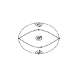
Figure 6. Phase portrait of Case $4$: $a_{1}=a_{2}=0$ and $a_{4}=0$.

Now we prove statement $(d)$. If $X$ has a semi–hyperbolic singularity then, by definition, for determining its phase portrait we have to study system (15) with $a_{4}+a_{8}\neq 0$ and $a_{4}a_{8}-a_{5}a_{7}=0$. We can divided the proof in three cases. First case $a_{4}=a_{5}=0$ and so $a_{8}\neq 0$. Second case $a_{4}=a_{7}=0$ and so $a_{8}\neq 0$. Third case $a_{8}=a_{5}a_{7}/a_{4}$ and $a_{4}\neq-a_{8}$. However, we need study only the first case because the last two cases are equivalent to it by a rotation of the variables. In fact, if the coefficients of $X$ satisfy the second or the third cases, then by the orthogonal linear change of variables $(x,y,z)=M_{i}(\tilde{x},\tilde{y},\tilde{z})$, $i=1,2$, where

$$M_{1}=\left(\begin{array}[]{ccc}\displaystyle-\frac{a_{8}}{\sqrt{a_{5}^{2}+a_{8}^{2}}}&\displaystyle\frac{a_{5}}{\sqrt{a_{5}^{2}+a_{8}^{2}}}&0\\ \displaystyle\frac{a_{5}}{\sqrt{a_{5}^{2}+a_{8}^{2}}}&\displaystyle\frac{a_{8}}{\sqrt{a_{5}^{2}+a_{8}^{2}}}&0\\ 0&0&1\end{array}\right)$$

and

$$M_{2}=\left(\begin{array}[]{ccc}\displaystyle-\frac{a_{7}}{\sqrt{a_{7}^{2}+a_{4}^{2}}}&\displaystyle\frac{a_{4}}{\sqrt{a_{7}^{2}+a_{4}^{2}}}&0\\ \displaystyle\frac{a_{4}}{\sqrt{a_{7}^{2}+a_{4}^{2}}}&\displaystyle\frac{a_{7}}{\sqrt{a_{7}^{2}+a_{4}^{2}}}&0\\ 0&0&1\end{array}\right),$$

the coefficients of $X$ in the variables $(\tilde{x},\tilde{y},\tilde{z})$ satisfy the first case, respectively. Thus, we suppose that $a_{4}=a_{5}=0$ and so $a_{8}\neq 0$. We distinguish the following four cases.

Case 5: $a_{1}a_{7}\neq 0$. We have that $X$ has only four singularities on $\mathbb{S}^{2}$, i.e. $(0,0,\pm 1)$,$(a_{7}/\sqrt{a_{7}^{2}+a_{1}^{2}},0,a_{1}/\sqrt{a_{7}^{2}+a_{1}^{2}})$ and $(-a_{7}/\sqrt{a_{7}^{2}+a_{1}^{2}},0,-a_{1}/\sqrt{a_{7}^{2}+a_{1}^{2}})$. These singularities correspond to the singularities $(0,0)$ and $(-a_{7}/a_{1},0)$ of system (15). Doing the change of variables $u=-a_{8}r/a_{7}$, $v=r+s$ and introducing the new time variable $\tau$ through $d\tau=-a_{8}dt$ system (15) can be written as

(33) $$\dot{r}=P_{2}(r,s),\;\;\dot{s}=s+Q_{2}(r,s).$$

If $a_{2}a_{7}-a_{1}a_{8}\neq 0$, we have that $\varphi(r)=((a_{2}a_{7}-a_{1}a_{8})(a_{7}^{2}+a_{8}^{2}))r^{2}/(a_{7}^{2}a_{8}^{2})+\cdots$ is the solution of $s+Q_{2}(r,s)=0$. Hence, $\psi(r)=P(r,\varphi(r))=(a_{2}a_{7}-a_{1}a_{8})r^{2}/a_{8}^{2}+\cdots$. Thus, by Theorem $65$ of page $340$ of [1], we have that $(0,0)$ is a saddle–node of system (33). Now, the trace and the determinant of the linear part from system (15) at $(-a_{7}/a_{1},0)$ are $(a_{2}a_{7}-a_{1}a_{8})/a_{1}$ and $a_{7}^{2}(a_{7}^{2}+a_{1}^{2})/a_{1}^{2}$, respectively. Therefore, $(-a_{7}/a_{1},0)$ can be a node or a focus of system (15). Now, by the orthogonal linear change of variables

$$\left(\begin{array}[]{c}x\\ y\\ z\end{array}\right)=\left(\begin{array}[]{ccc}0&\displaystyle\frac{a_{1}}{\sqrt{a_{1}^{2}+a_{7}^{2}}}&\displaystyle\frac{a_{7}}{\sqrt{a_{1}^{2}+a_{7}^{2}}}\\ 1&0&0\\ 0&-\displaystyle\frac{a_{7}}{\sqrt{a_{1}^{2}+a_{7}^{2}}}&\displaystyle\frac{a_{1}}{\sqrt{a_{1}^{2}+a_{7}^{2}}}\end{array}\right)\left(\begin{array}[]{c}\tilde{x}\\ \tilde{y}\\ \tilde{z}\end{array}\right),$$

the system associated to $X$ becomes

$$\begin{array}[]{lcl}\dot{\tilde{x}}&=&P(\tilde{x},\tilde{y},\tilde{z})=\displaystyle-\frac{a_{1}a_{2}+a_{7}a_{8}}{\sqrt{a_{1}^{2}+a_{7}^{2}}}\tilde{x}\tilde{y}-\frac{a_{2}a_{7}-a_{1}a_{8}}{\sqrt{a_{1}^{2}+a_{7}^{2}}}\tilde{x}\tilde{z}-a_{1}\tilde{y}^{2}-a_{7}\tilde{y}\tilde{z},\\ \dot{\tilde{y}}&=&Q(\tilde{x},\tilde{y},\tilde{z})=\displaystyle\frac{a_{1}a_{2}+a_{7}a_{8}}{\sqrt{a_{1}^{2}+a_{7}^{2}}}\tilde{x}^{2}+a_{1}\tilde{x}\tilde{y}+a_{7}\tilde{x}\tilde{z},\\ \dot{\tilde{z}}&=&R(\tilde{x},\tilde{y},\tilde{z})=\displaystyle\frac{a_{2}a_{7}-a_{1}a_{8}}{\sqrt{a_{1}^{2}+a_{7}^{2}}}\tilde{x}^{2}.\end{array}$$

Note that in these coordinates the singularity $(-a_{7}/(\sqrt{a_{1}^{2}+a_{7}^{2}}),0,-a_{1}/(\sqrt{a_{1}^{2}+a_{7}^{2}}))$ corresponds to the point $(0,0,-1)$. Hence, using the notation of Section 5, we have that $\tilde{R}(u,v)=R(2u,2v,u^{2}+v^{2}-1)=4(a_{2}a_{7}-a_{1}a_{8})/\sqrt{a_{1}^{2}+a_{7}^{2}}u^{2}$. Hence, $\tilde{R}$ does not change sign and by Theorem 3, $X$ does not have limit cycles on $\mathbb{S}^{2}$. So the phase portrait of $X$ on the Poincaré disc is equivalent to one of Figure 7. Note that the separatrices of the hyperbolic sectors of the diametrally opposite saddles–nodes can be connect or not, see Figures $5$ and $6$ of [11].

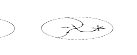
Figure 7. Phase portrait of Case $5$: $a_{1}a_{7}\neq 0$ and $a_{7}a_{2}-a_{8}a_{1}\neq 0$.

Now if $a_{7}a_{2}-a_{8}a_{1}=0$, system (33) has a straight line of singularities passing though the origin. Note that $H(x,y,z)=a_{7}x+a_{1}z$ is a first integral of $X$ and $\{H=0\}\cap\mathbb{S}^{2}$ is a circle of singularities. So the phase portrait of $X$ is equivalent to Figure 4 $(b)$.

Case 6: $a_{7}=0$ and $a_{1}\neq 0$. So $(0,0,\pm 1)$ are the unique singularities of $X$ on $\mathbb{S}^{2}$. Introducing the new time variable $\tau$ through $d\tau=-a_{8}dt$ system (15) can be written in the form

$$\dot{u}=P_{2}(u,v),\;\;\dot{v}=v+Q_{2}(u,v).$$

We have that $v=\varphi(u)=-a_{1}u^{2}/2a_{8}+\cdots$ is the solution of $v+Q_{2}(u,v)=0$. Hence, $\psi(u)=P(u,\varphi(u))=a_{1}^{2}u^{2}/a_{8}^{2}+\cdots$. Thus, by Theorem $65$ of page $340$ of [1], we have that $(0,0)$ is a topological node of system (15).

Now we consider the planar vector field induced by $X$ through the stereographic projection of (10) at the point $(0,0,1)$, i.e. we consider system (14) which in this case becomes

(34) $$\dot{r}=4a_{1}rs+4a_{2}s^{2}-4a_{8}rs^{2},\;\;\dot{s}=-2a_{8}s-4a_{1}r^{2}-4a_{2}rs+2a_{8}r^{2}s-2a_{8}s^{3}.$$

Since $\dot{s}\mid_{s=0}=-4a_{1}r^{2}$, the orbits of vector field determined by system (34) intersect the straight line $s=0$ always in a unique direction except at the point $(r,s)=(0,0)$, i.e $s=0$ is transversal to the flow of system (34) except at the origin. Thus, $X=(P,Q,R)$ does not have limit cycles on $\mathbb{S}^{2}$. We also can apply Theorem 3 of Section 5 to give another proof of this fact. Then, it is sufficient to see that $\tilde{R}(u,v)=R(2u,2v,u^{2}+v^{2}-1)=-4a_{8}v^{2}$ does not change sign. Hence, the phase portrait of $X$ on the Poincaré disc is equivalent to Figure 8.

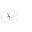
Figure 8. Phase portrait of Case $6$: $a_{7}=0$ and $a_{1}\neq 0$.

Case 7: $a_{7}=0$ and $a_{1}=0$. We have that $\{y=0\}\cap\mathbb{S}^{2}$ is a circle of singularities of $X$. As $H(x,y,z)=a_{8}x+a_{2}z$ is a first integral of $X$, it follows that phase portrait of $X$ is equivalent to Figure 4 $(a)$.

Case 8: $a_{7}\neq 0$ and $a_{1}=0$. Assume that $a_{2}\neq 0$, then $X$ has only four singularities on $\mathbb{S}^{2}$, $(0,0,\pm 1)$ and $(\pm 1,0,0)$. The singularities $(0,0,\pm 1)$ correspond to the singularity $(0,0)$ of system (15). Doing the change of variables $u=-a_{8}r/a_{7}$, $v=r+s$ and introducing the new time variable $\tau$ through $d\tau=-a_{8}dt$ system (15) can be written

(35) $$\dot{r}=P_{2}(r,s),\;\;\dot{s}=s+Q_{2}(r,s).$$

Since $a_{2}\neq 0$ we have that $s=\varphi(r)=(a_{2}(a_{7}^{2}+a_{8}^{2}))r^{2}/(a_{7}a_{8}^{2})+\cdots$ is the solution of $s+Q_{2}(r,s)=0$. Hence, $\psi(r)=P(r,\varphi(r))=(a_{7}a_{2})r^{2}/a_{8}^{2}+\cdots$. Thus, by Theorem $65$ of page $340$ of [1], we have that $(0,0)$ is a saddle–node of system (35). Now, the singularities $(\pm 1,0,0)$ have eigenvalues $\{0,-(a_{2}\pm\sqrt{a_{2}^{2}-4a_{7}^{2}})/2$ and $\{0,(a_{2}\pm\sqrt{a_{2}^{2}-4a_{7}^{2}})/2$, respectively. Therefore, $(\pm 1,0,0)$ can be nodes or foci of $X=(P,Q,R)$ restricted to $\mathbb{S}^{2}$. Now, using the notation of Section 5 and doing the change of variables $(x,y,z)\longmapsto(z,y,x)$, we have that $X$ becomes $(\mathcal{P},\mathcal{Q},\mathcal{R})=(R(z,y,x),Q(z,y,x),P(z,y,x))$ and so $\tilde{\mathcal{R}}(u,v)=P(u^{2}+v^{2}-1,2v,2u)=4a_{2}v^{2}$. Hence, $\tilde{\mathcal{R}}$ does not change sign and by Theorem 3, $X$ does not have limit cycles on $\mathbb{S}^{2}$. So the phase portrait of $X$ on the Poincaré disc is equivalent to one of Figures 9. Note that the separatrices of the hyperbolic sectors of the diametrally opposite saddles–nodes can be connect or not, see Figures $5$ and $6$ of [11].

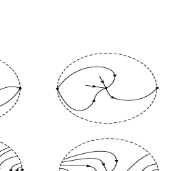
Figure 9. Phase portrait of Case $8$: $a_{7}a_{2}\neq 0$ and $a_{1}=0$.

Now if $a_{2}=0$, $X$ has a circle of singularities on $\mathbb{S}^{2}$ determined by the intersection of the plane $a_{7}x+a_{8}y=0$ with $\mathbb{S}^{2}$. Note that $H(x,y,z)=x$ is a first integral of $X$. So the phase portrait of $X$ is equivalent to Figure 4 $(a)$. $\Box$

Proof of Corollary 6. It is a straightforward consequence of the proof of Theorem 5. $\Box$

7. Singular points of homogeneous polynomial vector fields of $\mathbb{CP}^{2}$

In this section we present arguments and results which go back to Darboux [4], see also [3]. First we recall that $\mathbb{CP}^{2}=\{\mathbb{C}^{3}\setminus\{(0,0,0)\}\}/\thicksim$ with the equivalence relation $[X,Y,Z]\thicksim[X^{\prime},Y^{\prime},Z^{\prime}]$ if, and only if, there exists $\lambda\in\mathbb{C}\setminus\{0\}$ such that $[X^{\prime},Y^{\prime},Z^{\prime}]=\lambda[X,Y,Z]$.

Let $P$, $Q$ and $R$ be homogeneous polynomials of degree $m+1$ in the complex variables $X$, $Y$ and $Z$. We say that the homogeneous $1$–form $\omega=PdX+QdY+RdZ$ of degree $m+1$ is projective if $XP+YQ+ZR=0$. Therefore, the $1$–form is projective if and only if there exist three homogeneous polynomials $L$, $M$ and $N$ of degree $m$ such that $P=ZM-YN,\;Q=XN-ZL,\;R=YL-XM$, or equivalently $(P,Q,R)=(L,M,N)\land(X,Y,Z)$. Then we can write

$$\omega=\left|\begin{array}[]{ccc}L&M&N\\ X&Y&Z\\ dX&dY&dZ\end{array}\right|.$$

We notice that the polynomials $L$, $M$ and $N$ are not uniquely determined by $P$, $Q$ and $R$. These polynomials can be replaced by $L^{\prime}=L+X\Delta$, $M^{\prime}=M+Y\Delta$ and $N^{\prime}=N+Z\Delta$, where $\Delta$ is any homogeneous polynomial at the variables $X$, $Y$, $Z$ with degree $m-1$.

The projective $1$–form $\omega$ defines a differential equation in $\mathbb{CP}^{2}$ given by $\omega=0$, which may written as $(ZM-YN)dX+(XN-LZ)dY+(LY-MX)dZ=0$.

Usually in the literature a projective $1$–form $\omega$ is called a Pfaff algebraic form of degree $m+1$ of $\mathbb{CP}^{2}$, see for more details Jouanolou [12].

Let $F(X,Y,Z)$ be a homogeneous polynomial of degree $n$ in the variables $X$, $Y$, $Z$ and coefficients in $\mathbb{C}$. Then $F(X,Y,Z)=0$ is an algebraic curve of $\mathbb{CP}^{2}$. Let $p=(X_{0},Y_{0},Z_{0})$ be a point of $\mathbb{CP}^{2}$. Since the three coordinates of $p$ cannot be zero, without loss of generality we can assume that $p=(0,0,-1)$. Then suppose that the expression of $F(X,Y,Z)$ restricted to $Z=-1$ is

$$F(X,Y,-1)=F_{d}(X,Y)+F_{d+1}(X,Y)+\cdots+F_{n}(X,Y),$$

where $0\leq d\leq n$ and $F_{j}(X,Y)$ denotes a homogeneous polynomial of degree $j$ in the variables $X$ and $Y$ for $j=d,\ldots n$, with $F_{d}$ different from the zero polynomial. We say that $d=d_{p}(F)$ is the multiplicity of the curve $F=0$ at the point $p$. If $d=0$ then the point $p$ does not belong to the curve $F=0$. If $d=1$ we say that $p$ is a simple point for the curve $F=0$. If $d>1$ we say that $p$ is a multiple point of $F=0$. In particular $p$ is a multiple point of $F=0$ if and only if

$$\frac{\partial F}{\partial X}(p)=\frac{\partial F}{\partial Y}(p)=\frac{\partial F}{\partial Z}(p)=0.$$

Suppose that for $d>0$ we have that $F_{d}=\Pi_{i=1}^{r}L_{i}^{r_{i}}$ are different straight lines, called tangent lines to $F=0$ at the point $p$, $r_{i}$ is the multiplicity of the tangent line $L_{i}$ at $p$. For $d>1$ we say that $p$ is an ordinary multiple point if the multiplicity of all tangents at $p$ is $1$, otherwise we say that $p$ is a non–ordinary multiple point.

Let $F=0$ and $G=0$ be two algebraic curves and $p$ a point of $\mathbb{CP}^{2}$. We say that $F=0$ and $G=0$ intersect strictly at $p$, if $F=0$ and $G=0$ do not have any common component which pass through $p$. We say that $F=0$ and $G=0$ intersect transversally at $p$ if $p$ is a simple point of $F=0$ and $G=0$, and the tangent to $F=0$ at $p$ is distinct to the tangent to $G=0$ at $p$. The proof of the following two theorems can be found in [7].

Theorem 26.

(Intersection Number Theorem) There exists a unique multiplicity or intersection number $I(p,F\cap G)$ defined for all algebraic curves $F=0$ and $G=0$ and for all point $p$ of $\mathbb{CP}^{2}$ satisfying the following properties.

• $I(p,F\cap G)$ is a non–negative integer for all $F$, $G$ and $p$ when $F=0$ and $G=0$ intersect strictly at $p$. $I(p,F\cap G)=\infty$ if $F=0$ and $G=0$ do not intersect strictly at $p$.

• $I(p,F\cap G)=0$ if and only if $p$ is not a common point to $F=0$ and $G=0$. $I(p,F\cap G)$ depends only on the components of $F=0$ and $G=0$ which pass through $p$.

• If $T$ is a change of coordinates and $T(p)=q$, then $I(q,T(F)\cap T(G))=I(p,F\cap G)$.

• $I(p,F\cap G)=I(p,G\cap F)$.

• $I(p,F\cap G)\geq d_{p}(F)d_{p}(G)$, the equality holds if and only if $F=0$ and $G=0$ do not have common tangents at $p$.

• $I(p,F\cap G_{1}G_{2})=I(p,F\cap G_{1})+I(p,F\cap G_{2})$.

• $I(p,F\cap G)=I(p,F\cap(G+AF))$ for all homogeneous polynomial $A(X,Y,Z)$.

Theorem 27.

(Bezout Theorem) Let $F=0$ and $G=0$ be two algebraic curves of $\mathbb{CP}^{2}$ of degrees $r$ and $s$ respectively without common components. Then $\sum_{p}I(p,F\cap G)=rs$.

Let $F_{i}=0$, for $i=1,\ldots,s$, be algebraic curves and $p$ a point of $\mathbb{CP}^{2}$. We define the multiplicity or number of intersection of the curves $F_{1}=0,\ldots,F_{s}=0$ at $p$ as $I(p,\cap_{i=1}^{s}F_{i})=\min_{i<j}\{I(p,F_{i}\cap F_{j})\}$.

A point $[X_{0},Y_{0},Z_{0}]$ belonging to $\mathbb{CP}^{2}$ is a singular point of a projective $1$–form $\omega=PdX+QdY+RdZ$ of degree $m+1$ if $P(X_{0},Y_{0},Z_{0})=Q(X_{0},Y_{0},Z_{0})=R(X_{0},Y_{0},Z_{0})=0$, i.e. $[X_{0},Y_{0},Z_{0}]$ satisfies the system

$$ZM-YN=0,\;\;XN-ZL=0,\;\;YL-XM=0.$$

The proof of the next two results can be found in [4] or [17].

Lemma 28.

(Darboux Lemma) Let $A$, $A^{\prime}$, $B$, $B^{\prime}$, $C$ and $C^{\prime}$ be homogeneous polynomials in the variables $X$, $Y$ and $Z$ of degrees $l$, $l^{\prime}$, $m$, $m^{\prime}$, $n$ and $n^{\prime}$ respectively, verifying the identity $AA^{\prime}+BB^{\prime}+CC^{\prime}\equiv 0$. Assume that the curves $A=0$, $B=0$, $C=0$ and the curves $A^{\prime}=0$, $B^{\prime}=0$, $C^{\prime}=0$ do not have any common component, respectively. Then $\sum_{p}I(p,A\cap B\cap C)+\sum_{p}I(p,A^{\prime}\cap B^{\prime}\cap C^{\prime})=(lmn+l^{\prime}m^{\prime}n^{\prime})/\gamma$, where $\gamma=l+l^{\prime}=m+m^{\prime}=n+n^{\prime}$.

Proposition 29.

(Darboux Proposition) For any projective $1$–form of degree $m+1$ of $\mathbb{CP}^{2}$ having finitely many singular points we have that its number of singular points taking into account their multiplicities or numbers of intersection satisfies $\sum_{p}I(p,(ZM-YN)\cap(XN-ZL)\cap(YL-XM))=m^{2}+m+1$.

Proof of Theorem 7. We have that $X$ induce a projective $1$–form $\omega$ on $\mathbb{CP}^{2}$ of degree $n$ given by $\omega=PdX+QdY+RdZ$. Therefore, by the Darboux Proposition, $\omega$ has $(n-1)^{2}+(n-1)+1=n^{2}-n+1$ singular points, taking into account their multiplicities or numbers of intersection. Now, if $[X_{0},Y_{0},Z_{0}]$ is a singular point of $\omega$ and $(X_{0},Y_{0},Z_{0})\in\mathbb{R}^{3}$, then $\lambda(X_{0},Y_{0},Z_{0})$, $\lambda\in\mathbb{R}$, is a straight line of singular points of $X$ which determine exactly two singularities of $X$ on $\mathbb{S}^{2}$. Hence, we can conclude that if $X$ has finitely many singularities on $\mathbb{S}^{2}$, then $X$ has at most $2(n^{2}-n+1)$ singularities on $\mathbb{S}^{2}$. $\Box$

8. Topological classification of all phase portraits of homogeneous polynomial vector fields on $\mathbb{S}^{2}$ of degree $2$ modulo limit cycles

Let $X=(P,Q,R)$ be a homogeneous polynomial vector fields on $\mathbb{S}^{2}$ of degree $2$. Consider the system (3) associated to $X$. Using the notation of previous section, we can write (3) as

(36) $$\begin{array}[]{lcl}\dot{x}&=&z(a_{4}x+a_{5}y+a_{3}z)-y(-a_{1}x-a_{2}y)=zM-yN,\\ \dot{y}&=&x(-a_{1}x-a_{2}y)-z(-a_{7}x-a_{8}y-a_{6}z)=xN-zL,\\ \dot{z}&=&y(-a_{7}x-a_{8}y-a_{6}z)-x(a_{4}x+a_{5}y+a_{3}z)=yL-xM,\end{array}$$

where $L(x,y,z)=-a_{7}x-a_{8}y-a_{6}z$, $M(x,y,z)=a_{4}x+a_{5}y+a_{3}z$, $N(x,y,z)=-a_{1}x-a_{2}y$, i.e.

(37) $$\left(\begin{array}[]{c}L\\ M\\ N\end{array}\right)=\left(\begin{array}[]{ccc}-a_{7}&-a_{8}&-a_{6}\\ a_{4}&a_{5}&a_{3}\\ -a_{1}&-a_{2}&0\end{array}\right)\left(\begin{array}[]{c}x\\ y\\ z\end{array}\right)=A\left(\begin{array}[]{c}x\\ y\\ z\end{array}\right).$$

Note that $X=(P,Q,R)=(L,M,N)\land(x,y,z)$. Then, $(x_{0},y_{0},z_{0})\neq(0,0,0)$ is a singular point of $X$ if and only if there exist $\lambda_{0}\in\mathbb{R}$ such that $(L,M,N)(x_{0},y_{0},z_{0})=\lambda_{0}(x_{0},y_{0},z_{0})$. Now, as $L$, $M$ and $N$ are homogeneous polynomials, it follows that $\lambda(x_{0},y_{0},z_{0})$, $\lambda\in\mathbb{R}$, is a straight line of singularities of $X$. Therefore, for determining the singularities of $X$ we must find the real eigenvectors of the $3\times 3$ matrix $A$ given by (37), i.e. we have to calculate the real eigenvalues of $A$. Let $\lambda_{0}\in\mathbb{R}$ an eigenvalue of $A$. If there exists a unique eigenvector associated to $\lambda_{0}$, then it determines a straight line of singularities of $X$, and so we have two singularities of $X$ on $\mathbb{S}^{2}$. Now if there exist two eigenvectors associated to $\lambda_{0}$, then we have a plane of singularities of $X$ that determine a circle of singularities of $X$ on $\mathbb{S}^{2}$. Thus, $X$ has finitely many singularities on $\mathbb{S}^{2}$ if and only if each real eigenvalue of $A$ has exactly one eigenvector associated. Therefore, for degree $2$, we obtain another proof of Theorem 7. We also conclude that if $X$ has infinitely many singularities on $\mathbb{S}^{2}$, then it has one invariant circle on $\mathbb{S}^{2}$ formed by singularities and its phase portrait is equivalent to one of Figures 4 or 1.

In Section 6 we classified all phase portraits of homogeneous polynomial vector fields on $\mathbb{S}^{2}$ of degree $2$ having a degenerate singularity or a center. Therefore, for determining all phase portraits of a homogeneous polynomial vector field $X$ on $\mathbb{S}^{2}$ of degree $2$ we have to consider only the $X$’s with all their singularities non–degenerate and without centers. In this case, the singularities can be saddles, nodes or foci. Now, as these singularities have index $-1$ or $1$ and the maximum number of singularities of $X$ is $6$, by symmetry of $X$ with respect to origin and the Poincaré–Hopf Index Theorem (see, for instance [14]) it follows that we have to study the phase portraits with two saddles and four singularities that can be nodes or foci, and the phase portraits with two singularities that can be either nodes or foci.

Let $p$ be a singularity of $X$, by Proposition 14, we can suppose that $p=(0,0,-1)$ and so $a_{3}=a_{6}=0$ in (36). Hence,

$$A=\left(\begin{array}[]{ccc}-a_{7}&-a_{8}&0\\ a_{4}&a_{5}&0\\ -a_{1}&-a_{2}&0\end{array}\right).$$

We have that the eigenvalues of $A$ are $\{0,(a_{5}-a_{7}\pm\sqrt{\alpha})/2\}$, where $\alpha=(a_{5}+a_{7})^{2}-4a_{4}a_{8}$.

In the case that $X$ has only two singularities that can be either nodes or foci, then $A$ has either a unique eigenvalue with a unique eigenvector associated, or $A$ has one real eigenvalue and two complex eigenvalue. In the first case $0$ is the unique eigenvalue of $A$ and $0=(a_{5}-a_{7}+\sqrt{\alpha})(a_{5}-a_{7}-\sqrt{\alpha})=4(a_{4}a_{8}-a_{5}a_{7})$, i.e. $a_{4}a_{8}-a_{5}a_{7}=0$. Hence, using the notation of Section 6, we have that $(0,0,-1)$ is a degenerate singularity, because $\det(D\widetilde{X}(0,0))=a_{4}a_{8}-a_{5}a_{7}=0$. This case was already studied in Section 6.

If $A$ has one real eigenvalue and two complex, then $0$ is the real eigenvalue of $A$ and $\alpha<0$. Hence, as in this case the system associated to $X$ has the normal form (3) with $a_{3}=a_{6}=0$, we have that $\tilde{R}(u,v)=R(2u,2v,u^{2}+v^{2}-1)=-4(a_{4}u^{2}+(a_{5}+a_{7})uv+a_{8}v^{2})$. Solving $\tilde{R}=0$ with respect to $u$, it follows that $u=-(a_{5}+a_{7}\pm\sqrt{\alpha})v/(2a_{4})$ are its roots. Note that, as $\alpha<0$, $a_{4}\neq 0$. Thus we have that $(0,0)$ is the unique real root of $\tilde{R}=0$, and that $\tilde{R}$ does not change of sign. Therefore, applying Theorem 3 $(a)$, we have that in this case $X$ has no limit cycles and so its phase portrait in the Poincaré disc is equivalent to the one of Figure 8.

We have that $(0,0,-1)$ is a saddle of $X$ if and only if $\det(D\widetilde{X}(0,0))<0$, i.e. $a_{4}a_{8}-a_{5}a_{7}<0$. In this case, as $(a_{5}+a_{7})^{2}-4a_{4}a_{8}=(a_{5}-a_{7})^{2}-4(a_{4}a_{8}-a_{5}a_{7})>0$, $A$ has three reals eigenvalues given by $\{0,(a_{5}-a_{7}\pm\sqrt{\alpha})/2\}$. So $\alpha$ must be positive. Therefore, the eigenvectors of $A$ associated to the eigenvalues $\{0,(a_{5}-a_{7}\pm\sqrt{\alpha})/2\}$ are $(0,0,1)$, $((a_{8}(a_{5}-a_{7}+\sqrt{\alpha}))/(2a_{1}a_{8}-a_{2}(a_{5}+a_{7}+\sqrt{\alpha})),(a_{4}(a_{5}-a_{7}+\sqrt{\alpha}))/(2a_{2}a_{4}-a_{1}(a_{5}+a_{7}-\sqrt{\alpha})),1)$ and $((a_{8}(a_{5}-a_{7}-\sqrt{\alpha}))/(2a_{1}a_{8}-a_{2}(a_{5}+a_{7}-\sqrt{\alpha})),(a_{4}(a_{5}-a_{7}-\sqrt{\alpha}))/(2a_{2}a_{4}-a_{1}(a_{5}+a_{7}+\sqrt{\alpha})),1)$, respectively. Note that the eigenvectors of $A$ are well defined if $(2a_{1}a_{8}-a_{2}(a_{5}+a_{7}+\sqrt{\alpha}))(2a_{1}a_{8}-a_{2}(a_{5}+a_{7}-\sqrt{\alpha}))(2a_{2}a_{4}-a_{1}(a_{5}+a_{7}+\sqrt{\alpha}))(2a_{2}a_{4}-a_{1}(a_{5}+a_{7}-\sqrt{\alpha}))\neq 0$, i.e. if $16a_{4}a_{8}(a_{2}^{2}a_{4}-a_{1}a_{2}(a_{5}+a_{7})+a_{1}^{2}a_{8})^{2}\neq 0$. System (36) with $a_{3}=a_{6}=0$ and $a_{4}a_{8}-a_{5}a_{7}<0$ have two saddles and four singularities that can be nodes, foci or centers if and only if $A$ has three linearly independent eigenvectors. Thus, we distinguish the following cases.

Case 1: $16a_{4}a_{8}(a_{2}^{2}a_{4}-a_{1}a_{2}(a_{5}+a_{7})+a_{1}^{2}a_{8})^{2}\neq 0$. This case has been classified in the previous paragraph.

Case 2: $a_{4}=0$, $a_{1}\neq 0$ and $a_{2}(a_{5}+a_{7})-a_{1}a_{8}\neq 0$. In this case $-a_{5}a_{7}<0$ and the eigenvalues of $A$ are $0$, $-a_{7}$ and $a_{5}$ with respective eigenvectors $(0,0,1)$, $(a_{5}a_{8}/(a_{2}(a_{5}+a_{7})-a_{1}a_{8}),-a_{5}(a_{5}+a_{7})/(a_{2}(a_{5}+a_{7})-a_{1}a_{8}),1)$ and $(a_{7}/a_{1},0,1)$.

Case 3: $a_{4}=a_{1}=0$ and $a_{2}\neq 0$. In this case $-a_{5}a_{7}<0$ and so $a_{5}+a_{7}\neq 0$. The eigenvalues of $A$ are $0$, $-a_{7}$ and $a_{5}$ with respective eigenvectors $(0,0,1)$, $(1,0,0)$ and $(a_{5}a_{8}/(a_{2}(a_{5}+a_{7})),-a_{5}/a_{2},1)$.

Case 4: $a_{4}=a_{1}=a_{2}=0$. In this case $-a_{5}a_{7}<0$ and so $a_{5}+a_{7}\neq 0$. The eigenvalues of $A$ are $0$, $-a_{7}$ and $a_{5}$ with respective eigenvectors $(0,0,1)$, $(1,0,0)$ and $(-a_{8}/(a_{5}+a_{7}),1,0)$.

Case 5: $a_{4}=0$, $a_{1}\neq 0$ and $a_{8}=a_{2}(a_{7}+a_{5})/a_{1}$. Now the eigenvalues of $A$ are $0$, $-a_{7}$ and $a_{5}$ with respective eigenvectors $(0,0,1)$, $(a_{7}/a_{1},0,1)$ and $(-a_{2}/a_{1},1,0)$.

Case 6: $a_{1}=a_{2}=0$ and $a_{4}a_{8}\neq 0$. The eigenvalues of $A$ are $0$, $(a_{5}+a_{7}\pm\sqrt{\alpha})/2$ with respective eigenvectors $(0,0,1)$, $(-2a_{8}/(a_{5}+a_{7}+\sqrt{\alpha}),1,0)$ and $(-2a_{8}/(a_{5}+a_{7}-\sqrt{\alpha}),1,0)$.

Case 7: $a_{8}=a_{2}(-a_{2}a_{4}+a_{1}(a_{5}+a_{7}))/a_{1}^{2}$ and $a_{1}a_{4}\neq 0$. The eigenvalues of $A$ are $0$, $(a_{2}a_{4}-a_{1}a_{7})/a_{1}$ and $(a_{1}a_{5}-a_{2}a_{4})/a_{1}$ with respective eigenvectors $(0,0,1)$, $(((a_{1}a_{7}-a_{2}a_{4})(a_{1}(a_{5}+a_{7})-a_{2}a_{4}))/(a_{1}^{2}(a_{1}(a_{5}+a_{7})-2a_{2}a_{4})),((a_{2}a_{4}-a_{1}a_{7})a_{4})/(a_{1}(a_{1}(a_{5}+a_{7})-2a_{2}a_{4})),1)$ and $(-a_{2}/a_{1},1,0)$. Note that $a_{4}a_{8}-a_{5}a_{7}=(a_{2}a_{4}-a_{1}a_{5})(a_{1}a_{7}-a_{2}a_{4})/a_{1}^{2}<0$ and $a_{1}(a_{5}+a_{7})-2a_{2}a_{4}\neq 0$. Otherwise, $a_{5}=(2a_{2}a_{4}-a_{1}a_{7})/a_{1}$ and so $a_{4}a_{8}-a_{5}a_{7}=(a_{1}a_{7}-a_{2}a_{4})^{2}/a_{1}^{2}>0$.

Case 8: $a_{8}=0$. We have $-a_{5}a_{7}<0$. This case is equivalent to one of Cases $2$–$5$, i.e. if the coefficients of system (36) with $a_{3}=a_{6}=0$ satisfies $a_{8}=0$ then by the orthogonal linear change of variables

$$\left(\begin{array}[]{c}x\\ y\\ z\end{array}\right)=\left(\begin{array}[]{ccc}0&1&0\\ 1&0&0\\ 0&0&1\end{array}\right)\left(\begin{array}[]{c}\tilde{x}\\ \tilde{y}\\ \tilde{z}\end{array}\right)$$

we obtain one of Cases $2$–$5$.

Case $1$ is equivalent to Case $2$ doing the orthogonal linear change of variables $(x,y,z)=M(\tilde{x},\tilde{y},\tilde{z})$, where

$$M=\left(\begin{array}[]{ccc}\displaystyle-\frac{2a_{8}}{\sqrt{(a_{5}+a_{7}+\sqrt{\alpha})^{2}+4a_{8}^{2}}}&\displaystyle\frac{a_{5}+a_{7}+\sqrt{\alpha}}{\sqrt{(a_{5}+a_{7}+\sqrt{\alpha})^{2}+4a_{8}^{2}}}&0\\ \displaystyle\frac{a_{5}+a_{7}+\sqrt{\alpha}}{\sqrt{(a_{5}+a_{7}+\sqrt{\alpha})^{2}+4a_{8}^{2}}}&\displaystyle\frac{2a_{8}}{\sqrt{(a_{5}+a_{7}+\sqrt{\alpha})^{2}+4a_{8}^{2}}}&0\\ 0&0&1\end{array}\right),$$

and the $a_{i}$’s denote the coefficients of system (36) in the variables $(x,y,z)$ satisfying Case $1$. Indeed, denoting by $\tilde{a}_{i}$ the coefficients of system (36) in the variables $(\tilde{x},\tilde{y},\tilde{z})$, we have that $\tilde{a}_{1}=(2a_{1}a_{8}-a_{2}(a_{5}+a_{7}+\sqrt{\alpha}))/\sqrt{(a_{5}+a_{7}+\sqrt{\alpha})^{2}+4a_{8}^{2}}$, $\tilde{a}_{2}=-(2a_{2}a_{8}+a_{1}(a_{5}+a_{7}+\sqrt{\alpha}))/\sqrt{(a_{5}+a_{7}+\sqrt{\alpha})^{2}+4a_{8}^{2}}$, $\tilde{a}_{5}=1/2(a_{7}-a_{5}+\sqrt{\alpha})$, $\tilde{a}_{7}=1/2(a_{5}-a_{7}+\sqrt{\alpha})$, $\tilde{a}_{8}=a_{4}+a_{8}$, and $\tilde{a}_{3}=\tilde{a}_{4}=\tilde{a}_{6}=0$. Now, as $16a_{4}a_{8}(a_{2}^{2}a_{4}-a_{1}a_{2}(a_{5}+a_{7})+a_{1}^{2}a_{8})^{2}\neq 0$, it follows that $\tilde{a}_{4}=0$, $\tilde{a}_{1}\neq 0$, $\tilde{a}_{2}(\tilde{a}_{5}+\tilde{a}_{7})-\tilde{a}_{1}\tilde{a}_{8}\neq 0$ and $-\tilde{a}_{5}\tilde{a}_{7}=a_{4}a_{8}-a_{5}a_{7}<0$.

Case $6$ is equivalent to Case $4$ if $a_{5}+a_{7}\neq 0$ doing the orthogonal linear change of variables

$$\left(\begin{array}[]{c}x\\ y\\ z\end{array}\right)=\left(\begin{array}[]{ccc}a&b&0\\ d&e&0\\ 0&0&1\end{array}\right)\left(\begin{array}[]{c}\tilde{x}\\ \tilde{y}\\ \tilde{z}\end{array}\right),$$

where $a=((a_{5}+a_{7})^{2}(a_{4}+a_{8})+(a_{4}-a_{8})\sqrt{\sigma})/((a_{5}+a_{7})\sqrt{2\delta\beta})$, $b=((a_{5}+a_{7})(a_{5}(a_{5}+a_{7})^{2}-a_{4}(a_{8}(3a_{5}+a_{7})+a_{4}(a_{7}-a_{5})))-(a_{4}(a_{4}-a_{8})+a_{5}(a_{5}+a_{7}))\sqrt{\sigma})/(\sqrt{\delta\beta\gamma}$, $d=-\sqrt{\beta}/\sqrt{2\delta}$, $e=((a_{5}+a_{7})(a_{4}(2a_{8}(a_{4}-a_{8})-a_{7}(a_{5}+a_{7}))+a_{5}a_{8}(a_{5}+a_{7}))-(a_{7}a_{4}+a_{5}a_{8})\sqrt{\sigma})/\sqrt{\delta\beta\gamma}$, $\delta=(a_{5}+a_{7})^{2}+(a_{4}-a_{8})^{2}$, $\sigma=(a_{5}+a_{7})^{2}\alpha$, $\beta=(a_{5}+a_{7})^{2}+2a_{4}(a_{4}-a_{8})-\sqrt{\sigma}$, $\gamma=(a_{5}+a_{7})^{2}(a_{5}^{2}+a_{7}^{2}-2a_{4}a_{8})+(a_{7}^{2}-a_{5}^{2})\sqrt{\sigma}$, and the $a_{i}$’s denote the coefficients of system (36) in the variables $(x,y,z)$ satisfying Case $6$. Note that in this case $\delta>0$, $\sigma>0$. Now, as $((a_{5}+a_{7})^{2}+2a_{4}(a_{4}-a_{8})-\sqrt{\sigma})\cdot((a_{5}+a_{7})^{2}+2a_{4}(a_{4}-a_{8})+\sqrt{\sigma})=4a_{4}^{2}\delta$, $((a_{5}+a_{7})^{2}(a_{5}^{2}+a_{7}^{2}-2a_{4}a_{8})+(a_{7}^{2}-a_{5}^{2})\sqrt{\sigma})\cdot((a_{5}+a_{7})^{2}(a_{5}^{2}+a_{7}^{2}-2a_{4}a_{8})-(a_{7}^{2}-a_{5}^{2})\sqrt{\sigma})=4(a_{5}+a_{7})^{4}(a_{4}a_{8}-a_{5}a_{7})^{2}$, $(a_{5}+a_{7})^{2}+2a_{4}(a_{4}-a_{8})=a_{5}^{2}+a_{7}^{2}+2a_{4}^{2}-2(a_{4}a_{8}-a_{5}a_{7})>0$ and $a_{5}^{2}+a_{7}^{2}-2a_{4}a_{8}=(a_{5}-a_{7})^{2}-2(a_{4}a_{8}-a_{5}a_{7})>0$ it follows that $\beta>0$ and $\gamma>0$. Denoting by $\tilde{a}_{i}$ the coefficients of system (36) in the variables $(\tilde{x},\tilde{y},\tilde{z})$, we have that $\tilde{a}_{5}=-\sqrt{2}(a_{5}+a_{7})(a_{5}a_{7}-a_{4}a_{8})/\sqrt{\gamma}$, $\tilde{a}_{7}=-\sqrt{\gamma}/(2(a_{5}+a_{7}))$, $\tilde{a}_{8}=a_{4}+a_{8}$, $\tilde{a}_{1}=\tilde{a}_{2}=\tilde{a}_{4}=\tilde{a}_{3}=\tilde{a}_{4}=\tilde{a}_{6}=0$. Moreover, $-\tilde{a}_{5}\tilde{a}_{7}<0$.

Now, Case $6$ is equivalent to Case $4$ if $a_{7}=-a_{5}$ doing the orthogonal linear change of variables

$$\left(\begin{array}[]{c}x\\ y\\ z\end{array}\right)=\left(\begin{array}[]{ccc}\displaystyle\frac{\sqrt{a_{8}^{2}-a_{4}a_{8}}}{a_{4}-a_{8}}&\displaystyle\frac{a_{4}\sqrt{a_{8}^{2}-a_{4}a_{8}}+a_{5}\sqrt{a_{4}^{2}-a_{4}a_{8}}}{\sqrt{(a_{5}(a_{4}-a_{8})+\sqrt{-(a_{4}-a_{8})^{2}a_{4}a_{8}})^{2}}}&0\\ \displaystyle\frac{\sqrt{a_{4}^{2}-a_{4}a_{8}}}{a_{4}-a_{8}}&\displaystyle\frac{a_{8}\sqrt{a_{4}^{2}-a_{4}a_{8}}-a_{5}\sqrt{a_{8}^{2}-a_{4}a_{8}}}{\sqrt{(a_{5}(a_{4}-a_{8})+\sqrt{-(a_{4}-a_{8})^{2}a_{4}a_{8}})^{2}}}&0\\ 0&0&1\end{array}\right)\left(\begin{array}[]{c}\tilde{x}\\ \tilde{y}\\ \tilde{z}\end{array}\right).$$

Indeed, denoting by $\tilde{a}_{i}$ the coefficients of system (36) in the variables $(\tilde{x},\tilde{y},\tilde{z})$, we have that $\tilde{a}_{5}=(a_{5}^{2}+a_{8}a_{4})(a_{8}-a_{4})/\sqrt{(a_{5}(a_{4}-a_{8})+\sqrt{-(a_{4}-a_{8})^{2}a_{4}a_{8}})^{2}}$, $\tilde{a}_{7}=\sqrt{(a_{5}(a_{4}-a_{8})+\sqrt{-(a_{4}-a_{8})^{2}a_{4}a_{8}})^{2}}/(a_{4}-a_{8})$, $\tilde{a}_{8}=a_{4}+a_{8}$ and $\tilde{a}_{1}=\tilde{a}_{2}=\tilde{a}_{3}=\tilde{a}_{4}=\tilde{a}_{6}=0$. Now, since $a_{5}^{2}+a_{8}a_{4}<0$, it follows that $-\tilde{a}_{5}\tilde{a}_{7}<0$.

Case $3$ is equivalent to Case $5$ doing the orthogonal linear change of variables

$$\left(\begin{array}[]{c}x\\ y\\ z\end{array}\right)=\left(\begin{array}[]{ccc}\displaystyle-\frac{a_{8}}{\sqrt{(a_{5}+a_{7})^{2}+a_{8}^{2}}}&\displaystyle\frac{a_{5}+a_{7}}{\sqrt{(a_{5}+a_{7})^{2}+a_{8}^{2}}}&0\\ \displaystyle\frac{a_{5}+a_{7}}{\sqrt{(a_{5}+a_{7})^{2}+a_{8}^{2}}}&\displaystyle\frac{a_{8}}{\sqrt{(a_{5}+a_{7})^{2}+a_{8}^{2}}}&0\\ 0&0&1\end{array}\right)\left(\begin{array}[]{c}\tilde{x}\\ \tilde{y}\\ \tilde{z}\end{array}\right),$$

where the $a_{i}$’s denote the coefficients of system (36) in the variables $(x,y,z)$ satisfying Case $3$. Indeed, denoting by $\tilde{a}_{i}$ the coefficients of system (36) in the variables $(\tilde{x},\tilde{y},\tilde{z})$, we have that $\tilde{a}_{1}=-a_{2}(a_{5}+a_{7})/\sqrt{(a_{5}+a_{7})^{2}+a_{8}^{2}}$, $\tilde{a}_{2}=-a_{2}a_{8}/\sqrt{(a_{5}+a_{7})^{2}+a_{8}^{2}}$, $\tilde{a}_{5}=a_{7}$, $\tilde{a}_{7}=a_{5}$, $\tilde{a}_{8}=\tilde{a}_{2}(\tilde{a}_{5}+\tilde{a}_{7})/\tilde{a}_{1}$ and $\tilde{a}_{3}=\tilde{a}_{4}=\tilde{a}_{6}=0$. Now, as $a_{2}\neq 0$ and $-a_{5}a_{7}<0$, it follows that $\tilde{a}_{1}\neq 0$ and $-\tilde{a}_{5}\tilde{a}_{7}<0$.

Case $7$ is equivalent to Case $5$ doing the orthogonal linear change of variables $(x,y,z)=M(\tilde{x},\tilde{y},\tilde{z})$ with $M$ given by

$$\left(\begin{array}[]{ccc}\displaystyle\frac{a_{2}a_{4}-a_{1}(a_{5}+a_{7})}{\sqrt{(a_{1}(a_{5}+a_{7})-a_{2}a_{4})^{2}+a_{1}^{2}a_{4}^{2}}}&\displaystyle\frac{a_{4}a_{1}}{\sqrt{(a_{1}(a_{5}+a_{7})-a_{2}a_{4})^{2}+a_{1}^{2}a_{4}^{2}}}&0\\ \displaystyle\frac{a_{4}a_{1}}{\sqrt{(a_{1}(a_{5}+a_{7})-a_{2}a_{4})^{2}+a_{1}^{2}a_{4}^{2}}}&\displaystyle-\frac{a_{2}a_{4}-a_{1}(a_{5}+a_{7})}{\sqrt{(a_{1}(a_{5}+a_{7})-a_{2}a_{4})^{2}+a_{1}^{2}a_{4}^{2}}}&0\\ 0&0&1\end{array}\right),$$

where the $a_{i}$’s denote the coefficients of system (36) in the variables $(x,y,z)$ satisfying Case $3$. Note that, as $a_{1}\neq 0$ and $a_{4}a_{8}-a_{5}a_{7}=(a_{2}a_{4}-a_{1}a_{5})(a_{1}a_{7}-a_{2}a_{4})/a_{1}^{2}<0$, it follows that $(a_{1}(a_{5}+a_{7})-a_{2}a_{4})^{2}+a_{1}^{2}a_{4}^{2}\neq 0$. Denoting by $\tilde{a}_{i}$ the coefficients of system (36) in the variables $(\tilde{x},\tilde{y},\tilde{z})$, we have that $\tilde{a}_{1}=(a_{1}(a_{5}+a_{7})-2a_{2}a_{4})a_{1}/\sqrt{(a_{1}(a_{5}+a_{7})-a_{2}a_{4})^{2}+a_{1}^{2}a_{4}^{2}}$, $\tilde{a}_{2}=(a_{4}(a_{2}^{2}-a_{1}^{2})-a_{1}a_{2}(a_{5}+a_{7}))/\sqrt{(a_{1}(a_{5}+a_{7})-a_{2}a_{4})^{2}+a_{1}^{2}a_{4}^{2}}$, $\tilde{a}_{5}=(a_{2}a_{4}-a_{1}a_{5})/a_{1}$, $\tilde{a}_{7}=(a_{2}a_{4}-a_{1}a_{7})/a_{1}$, $\tilde{a}_{8}=\tilde{a}_{2}(\tilde{a}_{5}+\tilde{a}_{7})/\tilde{a}_{1}$, and $\tilde{a}_{3}=\tilde{a}_{4}=\tilde{a}_{6}=0$. Now, as $a_{1}(a_{5}+a_{7})-2a_{2}a_{4}\neq 0$, it follows that $\tilde{a}_{1}\neq 0$. Moreover, $-\tilde{a}_{5}\tilde{a}_{7}=(a_{2}a_{4}-a_{1}a_{5})(a_{1}a_{7}-a_{2}a_{4})/a_{1}^{2}<0$.

We conclude that for determining all phase portraits of all homogeneous polynomial vector field on $\mathbb{S}^{2}$ of degree $2$ having two saddles and four singularities that can be nodes, foci or centers we have to consider only Case $2$, $4$ and $5$, i.e. we have to consider the following families

(38) $$\begin{array}[]{lcl}\dot{x}&=&a_{5}yz-y(-a_{1}x-a_{2}y),\\ \dot{y}&=&x(-a_{1}x-a_{2}y)-z(-a_{7}x-a_{8}y),\\ \dot{z}&=&y(-a_{7}x-a_{8}y)-a_{5}xy,\end{array}$$

with $a_{1}\neq 0$, $a_{2}(a_{5}+a_{7})-a_{1}a_{8}\neq 0$ and $-a_{5}a_{7}<0$;

(39) $$\dot{x}=b_{5}yz,\;\;\dot{y}=-z(-b_{7}x-b_{8}y),\;\;\dot{z}=y(-b_{7}x-b_{8}y)-b_{5}xy,$$

with $-b_{5}b_{7}<0$; and

(40) $$\begin{array}[]{lcl}\dot{x}&=&c_{5}yz-y(-c_{1}x-c_{2}y),\\ \dot{y}&=&x(-c_{1}x-c_{2}y)-z\left(-c_{7}x-\displaystyle\frac{c_{2}(c_{5}+c_{7})}{c_{1}}y\right),\\ \dot{z}&=&y\left(-c_{7}x-\displaystyle\frac{c_{2}(c_{5}+c_{7})}{c_{1}}y\right)-c_{5}xy,\end{array}$$

with $c_{1}\neq 0$ and $-c_{5}c_{7}<0$.

Consider the vector field $X$ determined by system (39). Doing the orthogonal linear change of variables

$$\left(\begin{array}[]{c}x\\ y\\ z\end{array}\right)=\left(\begin{array}[]{ccc}0&0&1\\ 0&1&0\\ 1&0&0\end{array}\right)\left(\begin{array}[]{c}\bar{x}\\ \bar{y}\\ \bar{z}\end{array}\right),$$

system (39) becomes

(41) $$\dot{\bar{x}}=-b_{8}\bar{y}^{2}-(b_{5}+b_{7})\bar{y}\bar{z},\;\;\dot{\bar{y}}=b_{8}\bar{x}\bar{y}+b_{7}\bar{x}\bar{z},\;\;\dot{\bar{z}}=b_{5}\bar{x}\bar{y}.$$

Note that for $a_{2}=-b_{8}$, $a_{5}=-(b_{5}+b_{7})$ and $a_{7}=b_{7}$ system (41) becomes the system of Case $3$ in the proof of Theorem 5 of Section 6 with $a_{7}^{2}+a_{5}a_{7}<0$.

Now we will study the possible connections of separatrices of families (38) and (40) on $\mathbb{S}^{2}$. We have consider only the homoclinic orbits, because as the saddles of families (38) and (40) on $\mathbb{S}^{2}$ are diametrally opposite, by Proposition 12, if $X$ has a heteroclinic orbit on $\mathbb{S}^{2}$, then $X$ has an invariant circle on $\mathbb{S}^{2}$. Then, the phase portraits of homogeneous polynomial vector fields on $\mathbb{S}^{2}$ of degree $2$ having invariant circles have been classified in [11].

We saw that families (38) and (40) have six singularities, two saddles and other four singularities that can be nodes, foci or centers. Therefore, the homoclinic orbits that can appear in families (38) and (40) on $\mathbb{S}^{2}$ must be one of the described in Figures 10 (a) and (c).

\psfrag{A}[l][B]{$(a)$}\psfrag{B}[l][B]{$(b)$}\psfrag{C}[l][B]{$(c)$}\includegraphics[height=43.36243pt,width=216.81pt]{FigT17.eps}

Figure 10. Homoclinic orbits. The symbol $\bullet$ denotes a focus, a center or a node

Proposition 30.

Let $X$ be a homogeneous polynomial vector field of degree $2$. Then $X$ cannot realize Figure 10 $(b)$ or $(c)$.

Proof.

Suppose that $X$ realizes some of Figures 10 $(b)$ or $(c)$. We can suppose without loss of generality that the three singularities of Figure 10 $(b)$ or $(c)$ are in the southern hemisphere. We consider a great circle on $\mathbb{S}^{2}$ that contains the saddle and another great circle that contains the other two singularities. The great circle through the saddle is chosen in a such way that the two straight lines determined by these great circles through the central projection (4) in the tangent plane to $\mathbb{S}^{2}$ at the point $(0,0,-1)$ are parallel. Eventually these two great circles can coincide. Now, there exists a different great circle $C$ such that the straight line determined by it is also parallel to the previous straight lines, it does not contain the saddle point and the other two singularities belong to the half–sphere determined by it and containing the saddle point. As the orbits of $X$ are symmetric with respect to the origin, these three invariant circles cannot intersect in two singular opposite points. Moreover, we can choose $C$ such that the straight line determined by it is sufficiently close to the straight line that contains the saddle point, and $C$ intersects transversally the homoclinic orbits in four points (see Figure 11). Note that, as the orbits of $X$ are symmetric with respect to the origin, $C$ has six tangent points with orbits of $X$. But this is a contradiction with Proposition 23. Therefore, the phase portrait of $X$ cannot realize Figure 10 $(b)$ or $(c)$. ∎

\psfrag{B}[l][B]{$C$}\includegraphics[height=57.81621pt,width=144.54pt]{FigT18.eps}

Figure 11. The study of cases (b) and (c) of Figure 10

From Figure 5 we can see that there exist homogeneous polynomial vector fields on $\mathbb{S}^{2}$ of degree $2$ having a homoclinic orbit of the type described in Figure 10 $(a)$, where the singularity inside the loop is a center. However, we do not have examples where this singularity is a focus or a node, but numerical computation show that they exist. For example, we can consider the following family of homogeneous polynomial vector fields on $\mathbb{S}^{2}$ of degree $2$ determined by the system

(42) $$\dot{x}=-xy-2y^{2}+yz,\;\;\dot{y}=x^{2}+2xy+xz+a_{8}yz,\;\;\dot{z}=-2xy-a_{8}y^{2},$$

with $a_{8}\neq 4$. System (42) is obtained from (38) substituting $a_{1}=-1$, $a_{2}=-2$, $a_{5}=1$ and $a_{7}=1$. Now, consider the system induced by (42) through the central projection on the tangent plane to $\mathbb{S}^{2}$ at $(1,0,0)$, i.e. system (9) becomes

(43) $$\begin{array}[]{lcl}\dot{u}&=&-v-uv-2v^{2}-2u^{2}v-a_{8}uv^{2},\\ \dot{v}&=&-u-a_{8}v+u^{2}+2uv-2uv^{2}-a_{8}v^{3}.\end{array}$$

This system has three singularities, $(0,0)$, $(1,0)$ and $(-a_{8}/(a_{8}-4),2/(a_{8}-4))$ with respective eigenvalues $(-a_{8}\pm\sqrt{a_{8}^{2}+4})/2$, $(2-a_{8}\pm\sqrt{(2-a_{8})^{2}-16})/2$ and $(a_{8}^{2}-2a_{8}+2\pm\sqrt{(a_{8}^{2}-2a_{8}+2)^{2}-8(a_{8}^{2}+(a_{8}-4)^{2}+4)})/(2(4-a_{8}))$. Using the software $P4$, we can obtain the phase portraits of system (43) in the Poincaré disc. Thus, for $a_{8}=8/5$ and $a_{8}=9/5$ we obtain the phase portraits given by Figures 12 $(a)$ and $(b)$, respectively.

\psfrag{B}[l][B]{$(a)$}\psfrag{C}[l][B]{$(b)$}\includegraphics[height=57.81621pt,width=122.85876pt]{loop1T.eps}

Figure 12. Phase portrait of system (43).

In Figure 12 we have that $(0,0)$ is a saddle and $(1,0)$, $(-a_{8}/(a_{8}-4),2/(a_{8}-4))$ are unstable foci. Note that in Figure 12 $(a)$ one of the stable separatrices of $(0,0)$ emerges from the unstable focus $(1,0)$. Now, in Figure 12 $(b)$ one of the unstable separatrices of $(0,0)$ tend to the unstable focus $(1,0)$. Therefore, there exists at least one limit cycle surrounding $(1,0)$. We can conclude by Figure 12 that there exists a value of the parameter $a_{8}$ belonging to the interval $(8/5,9/5)$ such that there is a homoclinic orbit surrounding the unstable focus $(1,0)$. In this homoclinic orbit borns a limit cycle because in Figure 12 $(b)$ the point $(1,0)$ is an unstable focus surrounded by an unstable separatrix coming from the saddle $(0,0)$. It seems that moving the parameter of the system this limit cycle ends in the Hopf bifurcation which takes place at the singular point $(1,0)$.

We can conclude that if $X$ is a homogeneous polynomial vector field of degree $2$ on $\mathbb{S}^{2}$ with all its singularities non–degenerate, then its phase portrait on $\mathbb{S}^{2}$ is topologically equivalent to one of the phase portraits on $\mathbb{S}^{2}$ given in Figures 13. This proves Theorem 8.

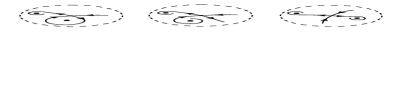
Figure 13. Phase portrait on the Poincaré disc of homogeneous polynomial vector fields on $\mathbb{S}^{2}$ of degree $2$ with a saddle. The symbol $\bullet$ denotes either a focus or a node surrounded perhaps by some limit cycles or a center. Note that the three singularities also can be surrounded by some limit cycles.

9. Hopf bifurcation on homogeneous polynomial vector fields on $\mathbb{S}^{2}$ of degree $2$

Let $X=(P,Q,R)$ be a homogeneous polynomial vector fields on $\mathbb{S}^{2}$ of degree $2$ and let $p$ be a singularity of $X$. Without loss of generality we can suppose that $p=(0,0,-1)$, because we can do a rotation of $SO(3)$ which preserves all the properties of $X$. Hence, using the notation of Section 6, the singularity $p$ is a weak focus of $X$ on $\mathbb{S}^{2}$ if $\mbox{tr}(D\tilde{X}(0,0))=0$, $\mbox{det}(D\tilde{X}(0,0))>0$ and $p$ is not a center.

Proposition 31.

Let $X$ be a homogeneous polynomial vector vector field on $\mathbb{S}^{2}$ and let $p=(0,0,-1)$ a singularity of $X$. Suppose that the system associated to $X$ is in the form (3) with $a_{3}=a_{6}=0$. Then $p$ is a weak focus of $X$ if and only if $a_{8}=-a_{4}$, $a_{4}^{2}+a_{7}a_{5}<0$ and $a_{4}(a_{1}^{2}-a_{2}^{2})+a_{1}a_{2}(a_{5}+a_{7})\neq 0$. Moreover, $p$ is stable if $a_{4}(a_{1}^{2}-a_{2}^{2})+a_{1}a_{2}(a_{5}+a_{7})<0$ and unstable if $a_{4}(a_{1}^{2}-a_{2}^{2})+a_{1}a_{2}(a_{5}+a_{7})>0$.

Proof.

The proof of this proposition follows directly of the proof of Theorem 2. ∎

Before stating the next theorem, we will state the Hopf Bifurcation Theorem.

Theorem 32.

(Hopf Bifurcation Theorem) Suppose that the analytical parame-trized system $\dot{x}=X(x,\mu)$, $x\in\mathbb{R}^{2}$, $\mu\in\mathbb{R}$, has a singular point at the origin for all values of the real parameter $\mu$. Furthermore, suppose that the eigenvalues, $\lambda_{1}(\mu)$ and $\lambda_{2}(\mu)$ of $DX(0,\mu)$, are pure imaginary for $\mu=\mu_{0}$. If the real part of the eigenvalues, $\mbox{Re}\lambda_{1}(\mu)=\mbox{Re}\lambda_{2}(\mu)$ in a neighborhood of $\mu_{0}$, satisfies $\displaystyle\frac{d}{d\mu}(\mbox{Re}\lambda_{1}(\mu))\mid_{\mu=\mu_{0}}>0$ and the origin is an asymptotically stable fixed point when $\mu=\mu_{0}$, then

• $\mu=\mu_{0}$ is a bifurcation point of the system;

• for $\mu\in(\mu_{1},\mu_{0})$, some $\mu_{1}<\mu_{0}$, the origin is a stable focus;

• for $\mu\in(\mu_{0},\mu_{2})$, some $\mu_{2}>\mu_{0}$, the origin is an unstable focus surrounded by a stable limit cycle, whose size increases with $\mu$.

The proof of Hopf Bifurcation Theorem can be found in [15].

Proof of Theorem 9. Consider the vector field $X=(P,Q,R)$ of the beginning of this section. By Sections 6 and 8, it follows that if $X$ has a weak focus, then the system associated to $X$ is equivalent to one of systems (38) or (40).

Consider system (40) with $c_{1}\neq 0$ and $-c_{5}c_{7}<0$. This system has six singularities, $(0,0,\pm 1)$, $(c_{7}/(\sqrt{c_{1}^{2}+c_{7}^{2}}),0,c_{1}/(\sqrt{c_{1}^{2}+c_{7}^{2}}))$, $(-c_{7}/(\sqrt{c_{1}^{2}+c_{7}^{2}}),0,-c_{1}/(\linebreak\sqrt{c_{1}^{2}+c_{7}^{2}}))$ and two singularities on $\mathbb{S}^{1}$, given by $(-c_{2}/(\sqrt{c_{2}^{2}+c_{1}^{2}}),c_{1}/(\sqrt{c_{2}^{2}+c_{1}^{2}}),0)$ and $(c_{2}/(\sqrt{c_{2}^{2}+c_{1}^{2}}),-c_{1}/(\sqrt{c_{2}^{2}+c_{1}^{2}}),0)$ with respective eigenvalues $\{0,(\sqrt{c_{2}^{2}+c_{1}^{2}}\pm\sqrt{c_{2}^{2}+c_{1}^{2}-4(c_{5}^{2}+c_{5}c_{7})})/2\}$, $\{0,(-\sqrt{c_{2}^{2}+c_{1}^{2}}\pm\sqrt{c_{2}^{2}+c_{1}^{2}-4(c_{5}^{2}+c_{5}c_{7})})/2\}$. As $c_{5}c_{7}\linebreak>0$, the singularities of $X$ on $\mathbb{S}^{1}$ are either nodes or strong foci on $\mathbb{S}^{2}$.

The planar system determined by system (40) through the central projection on the tangent plane to $\mathbb{S}^{2}$ at the point $(0,0,-1)$ is given by

$$\begin{array}[]{lcl}\dot{u}&=&\displaystyle-c_{5}v+c_{1}uv+c_{2}v^{2}-(c_{5}+c_{7})u^{2}v-\frac{c_{2}(c_{5}+c_{7})}{c_{1}}uv^{2},\\ \dot{v}&=&\displaystyle-c_{7}u-\frac{c_{2}(c_{5}+c_{7})}{c_{1}}v-c_{1}u^{2}-c_{2}uv-(c_{5}+c_{7})uv^{2}-\frac{c_{2}(c_{5}+c_{7})}{c_{1}}v^{3},\end{array}$$

see (9). This system has two singularities $(0,0)$ and $(-c_{7}/c_{1},0)$ corresponding to the singularities of $X$ that does not belong to $\mathbb{S}^{1}$. We saw, in Section 8, that $(0,0)$ is a saddle. Now, $(-c_{2}c_{5}\pm\sqrt{c_{2}^{2}c_{5}^{2}-4(c_{7}^{2}+c_{5}c_{7})(c_{1}^{2}+c_{7}^{2})})/2c_{1}$ are the eigenvalues of $(-c_{7}/c_{1},0)$. Again, as $c_{5}c_{7}>0$, a necessary condition in order that $(-c_{7}/c_{1},0)$ be a weak focus is $c_{2}=0$. If $c_{2}=0$, by the orthogonal linear change of variables

$$\left(\begin{array}[]{c}\tilde{x}\\ \tilde{y}\\ \tilde{z}\end{array}\right)=\left(\begin{array}[]{ccc}0&1&0\\ 1&0&0\\ 0&0&1\end{array}\right)\left(\begin{array}[]{c}x\\ y\\ z\end{array}\right),$$

system (40) becomes

$$\dot{\tilde{x}}=-c_{1}\tilde{y}^{2}+c_{7}\tilde{y}\tilde{z},\;\;\dot{\tilde{y}}=c_{1}\tilde{x}\tilde{y}+c_{5}\tilde{x}\tilde{z},\;\;\dot{\tilde{z}}=-(c_{5}+c_{7})\tilde{x}\tilde{y}.$$

This system satisfies Case $3$ in the proof of Theorem 5. Therefore, $(-c_{7}/\sqrt{c_{1}^{2}+c_{7}^{2}},0,\linebreak-c_{1}/(\sqrt{c_{1}^{2}+c_{7}^{2}})$ is a center of $X$ on $\mathbb{S}^{2}$ and the phase portrait of $X$ on $\mathbb{S}^{2}$ is equivalent to the phase portrait given by Figure 5 $(b)$ or $(c)$. Thus, in the family (40) its singularities cannot be weak foci and so it does not have a Hopf bifurcation.

Now we consider system (38). System (38) has six singularities, $(0,0,\pm 1)$, $(a_{5}a_{8}/\sqrt{\sigma},-a_{5}(a_{5}+a_{7})/\sqrt{\sigma},(a_{2}(a_{5}+a_{7})-a_{1}a_{8})/\sqrt{\sigma})$, $(-a_{5}a_{8}/\sqrt{\sigma},a_{5}(a_{5}+a_{7})/\sqrt{\sigma},\linebreak-(a_{2}(a_{5}+a_{7})-a_{1}a_{8})/\sqrt{\sigma})$, $(a_{7}/\sqrt{a_{7}^{2}+a_{1}^{2}},0,$ $a_{1}/\sqrt{a_{7}^{2}+a_{1}^{2}})$ and $(-a_{7}/\sqrt{a_{7}^{2}+a_{1}^{2}},0,\linebreak-a_{1}/\sqrt{a_{7}^{2}+a_{1}^{2}})$, where $\sigma=a_{5}^{2}(a_{8}^{2}+(a_{5}+a_{7})^{2})+(a_{2}(a_{5}+a_{7})-a_{1}a_{8})^{2}$. We saw in Section 8 that $(0,0,\pm 1)$ are saddles and the other four singularities can be nodes, foci or centers. By the orthogonal linear change of variables

$$\left(\begin{array}[]{c}\tilde{x}\\ \tilde{y}\\ \tilde{z}\end{array}\right)=\left(\begin{array}[]{ccc}0&1&0\\ \displaystyle\frac{a_{1}}{\sqrt{a_{1}^{2}+a_{7}^{2}}}&0&\displaystyle-\frac{a_{7}}{\sqrt{a_{1}^{2}+a_{7}^{2}}}\\ \displaystyle\frac{a_{7}}{\sqrt{a_{1}^{2}+a_{7}^{2}}}&0&\displaystyle\frac{a_{1}}{\sqrt{a_{1}^{2}+a_{7}^{2}}}\end{array}\right)\left(\begin{array}[]{c}x\\ y\\ z\end{array}\right),$$

system (38) becomes

$$\begin{array}[]{lcl}\dot{\tilde{x}}&=&\displaystyle-\frac{a_{1}a_{2}+a_{7}a_{8}}{\sqrt{a_{1}^{2}+a_{7}^{2}}}\tilde{x}\tilde{y}-\frac{a_{2}a_{7}-a_{1}a_{8}}{\sqrt{a_{1}^{2}+a_{7}^{2}}}\tilde{x}\tilde{z}-a_{1}\tilde{y}^{2}-a_{7}\tilde{y}\tilde{z},\\ \dot{\tilde{y}}&=&\displaystyle\frac{a_{1}a_{2}+a_{7}a_{8}}{\sqrt{a_{1}^{2}+a_{7}^{2}}}\tilde{x}^{2}+a_{1}\tilde{x}\tilde{y}+(a_{5}+a_{7})\tilde{x}\tilde{z},\\ \dot{\tilde{z}}&=&\displaystyle\frac{a_{2}a_{7}-a_{1}a_{8}}{\sqrt{a_{1}^{2}+a_{7}^{2}}}\tilde{x}^{2}-a_{5}\tilde{x}\tilde{y}.\end{array}$$

Note that in these coordinates the singularity $(-a_{7}/(\sqrt{a_{1}^{2}+a_{7}^{2}}),0,-a_{1}/(\sqrt{a_{1}^{2}+a_{7}^{2}}))$ goes over the point $(0,0,-1)$. Let $\tilde{a}_{1}=-(a_{1}a_{2}+a_{7}a_{8})/\sqrt{a_{1}^{2}+a_{7}^{2}}$, $\tilde{a}_{2}=-a_{1}$, $\tilde{a}_{4}=-(a_{2}a_{7}-a_{1}a_{8}/\sqrt{a_{1}^{2}+a_{7}^{2}}$, $\tilde{a}_{5}=-a_{7}$, $\tilde{a}_{7}=a_{5}+a_{7}$, and $\tilde{a}_{8}=0$. By Theorem 2, $(-a_{7}/\sqrt{a_{7}^{2}+a_{1}^{2}},0,-a_{1}/\sqrt{a_{7}^{2}+a_{1}^{2}})$ is a center of system (38) on $\mathbb{S}^{2}$ if $\tilde{a}_{4}=0$, i.e. $a_{2}a_{7}-a_{1}a_{8}=0$, $\tilde{a}_{4}^{2}+\tilde{a}_{5}\tilde{a}_{7}=-(a_{7}^{2}+a_{5}a_{7})<0$ and $\tilde{a}_{4}(\tilde{a}_{1}^{2}-\tilde{a}_{2}^{2})+\tilde{a}_{1}\tilde{a}_{2}(\tilde{a}_{5}+\tilde{a}_{7})=\sqrt{a_{1}^{2}+a_{2}^{2}}a_{1}a_{5}a_{8}/a_{7}=0$. However, this is not possible, because $a_{1}a_{5}a_{7}\neq 0$, $a_{2}a_{7}-a_{1}a_{8}=(\sqrt{a_{1}^{2}+a_{2}^{2}}a_{1}a_{5}a_{8})/a_{7}=0$ implies $a_{2}=a_{8}=0$, which is in contradiction with the hypothesis $a_{2}(a_{5}+a_{7})-a_{1}a_{8}\neq 0$. Therefore, $(-a_{7}/\sqrt{a_{7}^{2}+a_{1}^{2}},0,-a_{1}/\sqrt{a_{7}^{2}+a_{1}^{2}})$ cannot be a center. Now, if $a_{2}a_{7}-a_{1}a_{8}=0$, by Proposition 31 it is a weak focus of system (38).

The planar system determined by system (38) through the central projection on the tangent plane to $\mathbb{S}^{2}$ at the point $(0,0,-1)$ is

(44) $$\begin{array}[]{lcl}\dot{u}&=&\displaystyle-a_{5}v+a_{1}uv+a_{2}v^{2}-(a_{5}+a_{7})u^{2}v-a_{8}uv^{2},\\ \dot{v}&=&\displaystyle-a_{7}u-a_{8}v-a_{1}u^{2}-a_{2}uv-(a_{5}+a_{7})uv^{2}-a_{8}v^{3},\end{array}$$

see (9). This system has three singularities $(0,0)$, $(-a_{7}/a_{1},0)$ and$(-a_{5}a_{8}/(a_{2}(a_{5}+a_{7})-a_{1}a_{8}),a_{5}(a_{5}+a_{7})/(a_{2}(a_{5}+a_{7})-a_{1}a_{8}))$ corresponding to singularities of $X$ on $\mathbb{S}^{2}$. The singularity $(-a_{7}/a_{1},0)$ corresponds to singularity $(-a_{7}/\sqrt{a_{7}^{2}+a_{1}^{2}},0,-a_{1}/\sqrt{a_{7}^{2}+a_{1}^{2}})$ of system (38) on $\mathbb{S}^{2}$ and its eigenvalues are $\lambda_{\pm}(\mu)=(\mu\pm\sqrt{\mu^{2}-4(a_{7}^{2}+a_{5}a_{7})(a_{1}^{2}+a_{7}^{2})})/(2a_{1})$, where $\mu=-(a_{2}a_{7}-a_{1}a_{8})$. We saw that if $\mu=0$ and $\sqrt{a_{1}^{2}+a_{2}^{2}}a_{1}a_{5}a_{8}/a_{7}<0$, $(-a_{7}/a_{1},0)$ is a stable weak focus. Moreover, for $-2\sqrt{(a_{7}^{2}+a_{5}a_{7})(a_{1}^{2}+a_{7}^{2})}<\mu<2\sqrt{(a_{7}^{2}+a_{5}a_{7})(a_{1}^{2}+a_{7}^{2})}$ the singular point $(-a_{7}/a_{1},0)$ is a strong focus and $\displaystyle\frac{d}{d\mu}(\mbox{Re}\lambda_{\pm}(\mu))\mid_{\mu=0}=1$. Hence, by the Hopf Bifurcation Theorem, we have a Hopf bifurcation. This proves that there exist examples of homogeneous polynomial vector fields on $\mathbb{S}^{2}$ of degree $2$ with at least one limit cycle.

Now, consider the orthogonal linear change of variables $(\tilde{x},\tilde{y},\tilde{z})=M(x,y,z)$, where $M$ is the matrix

$$\left(\begin{array}[]{ccc}\displaystyle\frac{a_{5}+a_{7}}{\sqrt{(a_{5}+a_{7})^{2}+a_{8}^{2}}}&\displaystyle\frac{a_{8}(a_{2}(a_{5}+a_{7})-a_{1}a_{8})}{\sqrt{(a_{5}+a_{7})^{2}+a_{8}^{2}}\sqrt{\sigma}}&\displaystyle\frac{a_{5}a_{8}}{\sqrt{\sigma}}\\ \displaystyle\frac{a_{8}}{\sqrt{(a_{5}+a_{7})^{2}+a_{8}^{2}}}&\displaystyle-\frac{(a_{5}+a_{7})(a_{2}(a_{5}+a_{7})-a_{1}a_{8})}{\sqrt{(a_{5}+a_{7})^{2}+a_{8}^{2}}\sqrt{\sigma}}&\displaystyle-\frac{a_{5}(a_{5}+a_{7})}{\sqrt{\sigma}}\\ 0&\displaystyle-\frac{a_{5}\sqrt{(a_{5}+a_{7})^{2}+a_{8}^{2}}}{\sqrt{\sigma}}&\displaystyle\frac{a_{2}(a_{5}+a_{7})-a_{1}a_{8}}{\sqrt{\sigma}}\end{array}\right).$$

Hence, system (38) becomes

$$\begin{array}[]{lcl}\dot{\tilde{x}}&=&\tilde{a}_{1}\tilde{x}\tilde{y}+\tilde{a}_{2}\tilde{y}^{2}+\tilde{a}_{4}\tilde{x}\tilde{z}+\tilde{a}_{5}\tilde{y}\tilde{z},\\ \dot{\tilde{y}}&=&-\tilde{a}_{1}\tilde{x}^{2}-\tilde{a}_{2}\tilde{x}\tilde{y}+\tilde{a}_{7}\tilde{x}\tilde{z},\\ \dot{\tilde{z}}&=&-\tilde{a}_{4}\tilde{x}^{2}-(\tilde{a}_{5}+\tilde{a}_{7})\tilde{x}\tilde{y},\end{array}$$

where $\tilde{a}_{1}=-(a_{1}a_{2}((a_{5}+a_{7})^{2}-a_{8}^{2})+a_{8}(a_{5}a_{8}^{2}+(a_{5}+a_{7})(a_{2}^{2}-a_{1}^{2}+a_{5}(a_{5}+a_{7}))))/(\sqrt{(a_{5}+a_{7})^{2}+a_{8}^{2}}\sqrt{\sigma})$, $\tilde{a}_{2}=(a_{2}(a_{5}+a_{7})-a_{1}a_{2})/\sqrt{(a_{5}+a_{7})^{2}+a_{8}^{2}}$, $\tilde{a}_{4}=-(a_{8}(a_{2}a_{7}-a_{8}a_{1})-a_{1}(a_{5}^{2}+a_{5}a_{7}))/\sqrt{\sigma}$, $\tilde{a}_{5}=a_{5}$, and $\tilde{a}_{7}=-(a_{5}+a_{7})$. Note that in these coordinates the singularity $(-a_{5}a_{8}/\sqrt{\sigma},a_{5}(a_{5}+a_{7})/\sqrt{\sigma},-(a_{2}(a_{5}+a_{7})-a_{1}a_{8})/\sqrt{\sigma})$ becomes the point $(0,0,-1)$. By Theorem 2, $(-a_{5}a_{8}/\sqrt{\sigma},a_{5}(a_{5}+a_{7})/\sqrt{\sigma},-(a_{2}(a_{5}+a_{7})-a_{1}a_{8})/\sqrt{\sigma})$ is a center of system (38) on $\mathbb{S}^{2}$ if $\tilde{a}_{4}=0$, $\tilde{a}_{4}^{2}+\tilde{a}_{5}\tilde{a}_{7}<0$ and $\tilde{a}_{4}(\tilde{a}_{1}^{2}-\tilde{a}_{2}^{2})+\tilde{a}_{1}\tilde{a}_{2}(\tilde{a}_{5}+\tilde{a}_{7})=0$. We have that $\tilde{a}_{4}=0$ implies that $a_{8}(a_{2}a_{7}-a_{8}a_{1})-a_{1}(a_{5}^{2}+a_{5}a_{7})=0$. Note that in this case $a_{8}\neq 0$, otherwise $\tilde{a}_{4}=-a_{1}(a_{5}^{2}+a_{5}a_{7})/\sqrt{\sigma}\neq 0$. Hence, $a_{2}=a_{1}(a_{5}^{2}+a_{5}a_{7}+a_{8}^{2})/(a_{7}a_{8})$ and $\tilde{a}_{4}^{2}+\tilde{a}_{5}\tilde{a}_{7}=-(a_{5}^{2}+a_{5}a_{7})<0$, $\tilde{a}_{4}(\tilde{a}_{1}^{2}-\tilde{a}_{2}^{2})+\tilde{a}_{1}\tilde{a}_{2}(\tilde{a}_{5}+\tilde{a}_{7})=a_{1}\sqrt{a_{5}^{2}(a_{8}^{2}+(a_{5}+a_{7})^{2})(a_{1}^{2}(a_{5}+a_{7})^{2}+a_{8}^{2}(a_{1}^{2}+a_{7}^{2}))}/|a_{7}a_{8}|$. As $a_{1}\neq 0$, $(-a_{5}a_{8}/\linebreak\sqrt{\sigma},a_{5}(a_{5}+a_{7})/\sqrt{\sigma},-(a_{2}(a_{5}+a_{7})-a_{1}a_{8})/\sqrt{\sigma})$ cannot be a center. Now if $a_{8}(a_{2}a_{7}-a_{8}a_{1})-a_{1}(a_{5}^{2}+a_{5}a_{7})=0$, by Proposition 31 it is a weak focus of system (38).

The singularity $(-a_{5}a_{8}/(a_{2}(a_{5}+a_{7})-a_{1}a_{8}),a_{5}(a_{5}+a_{7})/(a_{2}(a_{5}+a_{7})-a_{1}a_{8}))$ of system (44) corresponds to the singularity $(-a_{5}a_{8}/\sqrt{\sigma},a_{5}(a_{5}+a_{7})/\sqrt{\sigma},-(a_{2}(a_{5}+a_{7})-a_{1}a_{8})/\sqrt{\sigma})$ of system (38) on $\mathbb{S}^{2}$ and its eigenvalues are $\lambda_{\pm}(\mu)=(\mu\pm\sqrt{\mu^{2}-4(a_{5}^{2}+a_{5}a_{7})\sigma})/(a_{2}(a_{5}+a_{7})-a_{1}a_{8})$, where $\mu=-(a_{8}(a_{2}a_{7}-a_{8}a_{1})-a_{1}(a_{5}^{2}+a_{5}a_{7}))$. We saw that if $\mu=0$ and $a_{1}/|a_{7}a_{8}|\sqrt{(a_{1}^{2}(a_{5}+a_{7})^{2}+a_{8}^{2}(a_{1}^{2}+a_{7}^{2}))}\cdot\linebreak\sqrt{a_{5}^{2}(a_{8}^{2}+(a_{5}+a_{7})^{2})}<0$, then $(-a_{5}a_{8}/(a_{2}(a_{5}+a_{7})-a_{1}a_{8}),a_{5}(a_{5}+a_{7})/(a_{2}(a_{5}+a_{7})-a_{1}a_{8}))$ is a stable weak focus. Moreover, for $-2\sqrt{(a_{5}^{2}+a_{5}a_{7})\sigma}<\mu<2\sqrt{(a_{5}^{2}+a_{5}a_{7})\sigma}$, $(-a_{5}a_{8}/(a_{2}(a_{5}+a_{7})-a_{1}a_{8}),a_{5}(a_{5}+a_{7})/(a_{2}(a_{5}+a_{7})-a_{1}a_{8}))$ is a strong focus and $\displaystyle\frac{d}{d\mu}(\mbox{Re}\lambda_{\pm}(\mu))\mid_{\mu=0}=1$. Hence, by the Hopf Bifurcation Theorem, we have a Hopf bifurcation. Note that system (38) cannot have two weak foci at the same time. $\Box$

10. Rotated vector field family

In this section, we summarize the behavior of the limit cycles in the special one–parameter family given by a rotated family of planar vector fields. The earliest work about these families can be found in the paper [5] of Duff in $1953$. Later on Seifert [18], Perko [16] and Chen Xiang–yan [19, 20, 21], etc successively improved the work of Duff.

Consider the vector fields $X_{\alpha}(x,y)=(P(x,y,\alpha),Q(x,y,\alpha))$ depending on the parameter $\alpha$. Suppose that when $\alpha$ varies on an interval $(a,b)$, the singular points of the vector fields $X_{\alpha}$ remain unchanged, and for any fixed point $p=(x,y)$ and any parameters $\alpha_{1}<\alpha_{2}\in(a,b)$, we have

(45) $$\left|\begin{array}[]{cc}P(x,y,\alpha_{1})&Q(x,y,\alpha_{1})\\ P(x,y,\alpha_{2})&Q(x,y,\alpha_{2})\end{array}\right|\geq 0\;(\mbox{or}\leq 0),$$

where the equality cannot hold on an entire periodic orbit of $X_{\alpha}$ with $\alpha=\alpha_{i}$, for $i=1,\;2$. Then, the family of vector fields $X_{\alpha}$ is called a ( generalized) rotated family with respect to the parameter $\alpha$. Here, the interval $(a,b)$ can be either bounded or unbounded.

The geometric meaning of condition (45) is the following. At any fixed point $p=(x,y)$, the oriented area between the vectors $(P(x,y,\alpha_{1}),Q(x,y,\alpha_{1}))$ and $(P(x,y,\alpha_{2}),Q(x,y,\alpha_{2}))$ has the same (or opposite) sign as sgn$(\alpha_{2}-\alpha_{1})$. That is, at any point $p=(x,y)$, as the parameter $\alpha$ increases, the vector $(P(x,y,\alpha),Q(x,y,\alpha))$ can only rotate in one direction; moreover, the angle of rotation cannot exceed $\pi$.

In the following we present four important results concerning periodic orbits and limit cycles for rotated vector field families $X_{\alpha}$.

• Non–intersection property: For distinct $\alpha_{1}$ and $\alpha_{2}$, the periodic orbits of the vector field $X_{\alpha}$ with $\alpha=\alpha_{1}$ and of the vector field $X_{\alpha}$ with $\alpha=\alpha_{2}$ cannot intersect.

• Stable and unstable property: When the parameter $\alpha$ changes slightly and monotonically, the stable and unstable limit cycle cannot disappear; it expands or contracts monotonically.

• Semiestable property: When the parameter $\alpha$ varies in the suitable direction, a semistable limit cycle bifurcates into one stable and one unstable limit cycle. When $\alpha$ varies in the opposite direction the semistable limit cycle disappears.

• Ending or starting property: When the parameter $\alpha$ varies a family of limit cycles only can disappears or appears either at a singular point, or in a semistable limit cycle, or in a separatrix cycle, or at infinity (i.e. the family becomes unbounded).

Consider system (40) with $c_{1}\neq 0$ and $-c_{5}c_{7}<0$. This system has six singularities, $(0,0,\pm 1)$, $(c_{7}/\sqrt{c_{1}^{2}+c_{7}^{2}},0,c_{1}/\sqrt{c_{1}^{2}+c_{7}^{2}})$, $(-c_{7}/\sqrt{c_{1}^{2}+c_{7}^{2}},0,-c_{1}/\sqrt{c_{1}^{2}+c_{7}^{2}})$ and two singularities on $\mathbb{S}^{1}$, given by $(-c_{2}/\sqrt{c_{2}^{2}+c_{1}^{2}},c_{1}/\sqrt{c_{2}^{2}+c_{1}^{2}},0)$ and $(c_{2}/\linebreak\sqrt{c_{2}^{2}+c_{1}^{2}},-c_{1}/\sqrt{c_{2}^{2}+c_{1}^{2}},0)$. We saw in the proof of Theorem 9 that the singularities of $X$ on $\mathbb{S}^{1}$ are either nodes or strong foci on $\mathbb{S}^{2}$.

Now we consider the planar system determined by system (40) through the central projection on the tangent plane to $\mathbb{S}^{2}$ at the point $(0,0,-1)$, i.e.

(46) $$\begin{array}[]{lcl}\dot{u}&=&\displaystyle-c_{5}v+c_{1}uv+c_{2}v^{2}-(c_{5}+c_{7})u^{2}v-\frac{c_{2}(c_{5}+c_{7})}{c_{1}}uv^{2},\\ \dot{v}&=&\displaystyle-c_{7}u-\frac{c_{2}(c_{5}+c_{7})}{c_{1}}v-c_{1}u^{2}-c_{2}uv-(c_{5}+c_{7})uv^{2}-\frac{c_{2}(c_{5}+c_{7})}{c_{1}}v^{3},\end{array}$$

see (9). This system has two singularities $(0,0)$ and $(-c_{7}/c_{1},0)$ corresponding to the singularities of $X$ that does not belong to $\mathbb{S}^{1}$. We saw, in Section 8, that $(0,0)$ is a saddle and, by the proof of Theorem 9, if $c_{2}=0$ then $(-c_{7}/c_{1},0)$ is a center; and if $c_{2}\neq 0$, then it is a node or a strong focus.

Proposition 33.

The vector field associated to system (46) does not have limit cycles.

Proof.

Consider the one parameter family of vector fields $(P(u,v,c_{2}),Q(u,v,c_{2}))$ associated to system (46). We have that

$$\left|\begin{array}[]{cc}P(u,v,c_{2})&Q(u,v,c_{2})\\ P(u,v,\tilde{c}_{2})&Q(u,v,\tilde{c}_{2})\end{array}\right|=(\tilde{c}_{2}-c_{2})\frac{c_{5}(c_{5}+c_{7})}{c_{1}}(1+u^{2}+v^{2})v^{2}.$$

Therefore, system (46) determines a rotated vector field family with respect to the parameter $c_{2}$. Now, note that for $c_{2}=0$, $(-c_{7}/c_{1},0)$ is a center of this family. Then, by the non–intersection property (i) and the ending or starting property (iv), system (46) does not have limit cycles. ∎

We conclude by Proposition 33 that if the vector field $X$ on $\mathbb{S}^{2}$ associated to system (40) with $c_{1}\neq 0$ and $-c_{5}c_{7}<0$ has a limit cycle, then this limit cycle surrounds one of the singularities that belongs to $\mathbb{S}^{1}$. These singularities always are nodes or strong foci. We believe that the following conjecture holds.

Conjecture The vector field associated to system (40) with $c_{1}\neq 0$ and $-c_{5}c_{7}<0$ does not have limit cycles on $\mathbb{S}^{2}$.

References

[1]A.A. Andronov, E.A. Leontovich, I.I. Gordon and A.G. Maier,
Qualitative theory of second-order dynamic systems, John Wiley &
Sons, .
[2]M.I. Camacho,
Geometric properties of homogeneous vector fields of degree two in
, Trans. Amer. Math. Soc.268 (1981),
79–101.
[3]J. Chavarriga and J. Llibre,
Invariant algebraic curves and rational first integrals for planar
polynomial vector fields, J. Differential Equations169 (2001), 1–16.
[4]G. Darboux, Mémoire sur les équations
différentielles algébrique du premier ordre et du premier
degré (Mélanges), Bull. Sci. Math. 2éme série, 2 (1878), 60–96; 123–144; 151–200.
[5]G. F. D. Duff, Limit cycles and rotated vector
fields, Ann. of Math.57 (1953), 15–31.
[6]T. Fukushima and T. Yamamoto,
A quasi–regularization of the Euler problem by partitioned
multistep methods, Proceedings of the 36th Symposium on
Celestial Mechanics, March 1–3, 2004 at Seiun–So, Hakone,
Kanagawa, Japan.
[7]W. Fulton, Algebraic curves, New York: W. A. Benjamin Inc., .
[8]H. Giacomini, J. Llibre and M. Viano,
On the nonexistence, existence and uniqueness of Limit cycles,
Nonlinearity9 (1996), 501–516.
[9]C. Gutierrez and J. Llibre,
Darbouxian integrability for polynomial vector fields on the
-dimensional sphere, Extracta Mathematicae17
(2002), 289–301.
[10]C. Lansun, Z. Xinan and L. Zhaojun,
Global topological properties of homogeneous vector fields in
, Chin. Ann. of Math., Ser. 20 B, 2
(1999), 185–194.
[11]J. Llibre and C. Pessoa,
Homogeneous polynomial vector fields of degree on the
–dimensional sphere, preprint, 2006.
[12]J. Llibre and C. Pessoa,
Invariant circles for homogeneous polynomial vector fields on the
–dimensional sphere, to appear in Rend. Cir. Mat.
Palermo, 2006.
[13]M. Makhaniok, J. Hesser, S. Noehte andR.
Männer, Limit cycles of a planar vector field, Acta
Applicandae Mathematicae 48 (1997), 12–32.
[14]J. W. Milnor,
Topology from the differentiable viewpoint, Princeton Landmarks in
Math., Princeton Universit Press, New Jersey 1997.
[15]J. E. Marsden and M. McCracken,
The Hopf bifurcation and its applications, Applied Mathematical
Sciences, Vol. 19, Springer, New York 1976.
[16]L. Perko, Rotated vector fields and the global behavior of limit
cycles for a class of quadratic systems in the plane, J.
Differential Equations18 (1975), 63–86.
[17]C. Pessoa,
Homogeneous polynomial vector fields on the –dimensional
sphere, Ph. D. thesis, Universitat Autònoma de Barcelona,
2006.
[18]G. Seifert, A rotated vector aproach to the problem of stability of
solutions of pendulum–type equations, in Contributions to the
theory of nonlinear oscilations, Annals of Math. Studies3 (1956), 1–16.
[19]C. Xiang–Yan, Applications of the theory of rotated vector fields
I, Nanjing Daxue Xuebao (Math.)1 (1963), 19–25.
[20]C. Xiang–Yan, Applications of the theory of rotated vector fields
II, Nanjing Daxue Xuebao (Math.)2 (1963), 43–50.