Finite-SNR Diversity-Multiplexing Tradeoff and Optimum Power Allocation in Bidirectional Cooperative Networks

Abstract

This paper focuses on analog network coding (ANC) and time division broadcasting (TDBC) which are two major protocols used in bidirectional cooperative networks. Lower bounds of the outage probabilities of those two protocols are derived first. Those lower bounds are extremely tight in the whole signal-to-noise ratio (SNR) range irrespective of the values of channel variances. Based on those lower bounds, finite-SNR diversity-multiplexing tradeoffs of the ANC and TDBC protocols are obtained. Secondly, we investigate how to efficiently use channel state information (CSI) in those two protocols. Specifically, an optimum power allocation scheme is proposed for the ANC protocol. It simultaneously minimizes the outage probability and maximizes the total mutual information of this protocol. For the TDBC protocol, an optimum method to combine the received signals at the relay terminal is developed under an equal power allocation assumption. This method minimizes the outage probability and maximizes the total mutual information of the TDBC protocol at the same time.

I Introduction

In traditional unidirectional cooperative networks, several relays assist in the communication between one source and one destination in order to achieve spatial diversity [1]. The diversity-multiplexing tradeoff, which is one of the most fundamental properties of any communication systems, of such networks has been extensively studied [2]–[6]. It has been shown that, in the unidirectional cooperative networks, the half-duplex constraint of every terminal induces a severe loss of bandwidth efficiency as demonstrated by a pre-log factor $1/2$ in the mutual information expression. In order to overcome this difficulty, bidirectional cooperative networks were studied in [7], where two sources exchanged information with the help of several relays. As a result, there were two traffic flows in a bidirectional cooperative network and they were supported by the same physical channels concurrently. Although each traffic flow still had the pre-log factor $1/2$ in its mutual information expression, the total mutual information of the network, which was the summation of the mutual information of both traffic flows, no longer suffered from the pre-log factor $1/2$. Therefore, bidirectional cooperative networks had much higher bandwidth efficiency than unidirectional cooperative networks.

Recently, many novel protocols were studied in the context of bidirectional cooperative networks, such as physical layer network coding (PNC) [8]–[10], analog network coding (ANC) [11], [12], and time division broadcast (TDBC) [8] and [13]–[15]. Those protocols not only achieved high bandwidth efficiency but also successfully controlled the interferences between the two traffic flows in a bidirectional cooperative network. Many previous works assumed that there was no direct channel between the two sources [8], [11], [12], and [15]–[19]. Under this assumption, the authors showed that the PNC and ANC protocols had larger capacity regions and higher sum-rates than the TDBC protocol [8], [11], and [19]. On the other hand, since there is no direct channel, the maximum diversity gains of the PNC, ANC, and TDBC protocols are the same, just one. Therefore, one may conclude that the PNC and ANC protocols always outperform the TDBC protocol in terms of diversity-multiplexing tradeoff [20].

In fact, numerous previous publications on cooperative networks have also considered the case that there is a direct channel between the two sources [1]–[3], [5], [6], [13], [14], and [21]–[23]. For this case, the comparison of diversity-multiplexing tradeoff might have different result. It is not hard to see that the TDBC protocol can utilize this direct channel [13], [14]; but the PNC and ANC protocols can not do so due to the half-duplex constraint [23]. Thus, the TDBC protocol might have a higher diversity gain than the PNC and ANC protocols. This is fundamentally different from the case where the direct channel does not exist. Therefore, it is necessary and interesting to compare those protocols in terms of diversity-multiplexing tradeoff under the assumption that the direct channel exists. Furthermore, it is more desirable to compare the tradeoff at finite signal-to-noise ratio (SNR) range as in [24] instead of only at infinite SNR in [20], because practical communication systems, such as wireless local area networks, usually work in the SNR range $3$–$20$ dB. However, such comparison has not been investigated in previous publications. This has motivated our work.

In this paper, we assume that the relays work in the amplify-and-forward mode, and hence, we do not consider the PNC protocol. In fact, it has been shown that the PNC protocol may suffer considerable performance loss in fading channels [19], [25]. Thus, we focus on the ANC and TDBC protocols in this paper. The contributions of this paper are summarized as follows:

• We derive lower bounds of the outage probabilities of the ANC and TDBC protocols. Those bounds are extremely tight in the whole SNR range, irrespective of the values of channel variances.

• We obtain the finite-SNR diversity-multiplexing tradeoffs of the ANC and TDBC protocols. Those tradeoffs establish a framework which enables us to make a comprehensive comparison between those two protocols. For example, the maximum diversity gain of the TDBC protocol is twice larger than that of the ANC protocol. However, the ANC protocol achieves a higher diversity gain when the multiplexing gain is larger than $1/2$, irrespective of the value of SNR.

• For the ANC protocol, we propose an optimum power allocation scheme which simultaneously minimizes the outage probability and maximizes the total mutual information of this protocol.

• For the TDBC protocol, we develop an optimum method to combine the received signals at the relay when equal power allocation is applied. This method simultaneously minimizes the outage probability and maximizes the total mutual information as well.

The rest of this paper is organized as follows. Section II describes the system models of the ANC and TDBC protocols. Section III focuses on the outage probabilities and finite-SNR diversity-multiplexing tradeoffs of those two protocols. In Section IV, we first develop an optimum power allocation scheme for the ANC protocol. Then we propose an optimum method for the TDBC protocol to combine the received signals at the relay. Section V presents some numerical results and Section VI concludes this paper.

II System Model

We consider a bidirectional cooperative network with two sources and one relay, where the sources intend to exchange information with the help of the relay. Every terminal has only one antenna and is half-duplex. We use ${\mathrm{S}}_{1}$, ${\mathrm{S}}_{2}$, and ${\mathrm{R}}$ to denote the first source, the second source, and the relay, respectively. Let $g$ represent the fading coefficient of the channel between ${\mathrm{S}}_{1}$ and ${\mathrm{S}}_{2}$, $h$ the channel between $\mathrm{S}_{1}$ and $\mathrm{R}$, and $f$ the channel between ${\mathrm{R}}$ and $\mathrm{S}_{2}$. Furthermore, we assume that $g$, $h$, and $f$ are complex Gaussian random variables with zero mean and variances $\Omega_{g}$, $\Omega_{h}$, and $\Omega_{f}$, respectively. The additive noise associated with every channel is assumed to be a complex Gaussian random variable with zero mean and unit variance. Let $x_{1}$ and $x_{2}$ denote the information-bearing symbol transmitted from ${\mathrm{S}}_{1}$ and ${\mathrm{S}}_{2}$, respectively. Both $x_{1}$ and $x_{2}$ have unit power. The total transmission power of the bidirectional cooperative network is constrained to be $3E$.

Since the two sources intend to exchange information, there are two traffic flows in this bidirectional cooperative network. One is from ${\mathrm{S}}_{1}$ via ${\mathrm{R}}$ to ${\mathrm{S}}_{2}$ and the other is from ${\mathrm{S}}_{2}$ via ${\mathrm{R}}$ to ${\mathrm{S}}_{1}$. Each traffic flow can be seen as a traditional unidirectional cooperative network. For example, in the first traffic flow, ${\mathrm{S}}_{1}$ is the transmitter, and ${\mathrm{R}}$ and ${\mathrm{S}}_{2}$ are the receivers. Hence, it is reasonable to assume that ${\mathrm{R}}$ knows $h$ and ${\mathrm{S}}_{2}$ knows $h$, $f$, and $g$ as in the conventional unidirectional cooperative networks [1], [21]. Similarly, due to the existence of the second traffic flow, it is reasonable to assume that ${\mathrm{R}}$ knows $f$ and ${\mathrm{S}}_{1}$ knows $h$, $f$, and $g$. In all, we assume that the two sources know $h$, $f$, and $g$, and the relay knows $h$ and $f$ as in many previous publications [7], [17], [18], and [26].

II-A Analog Network Coding (ANC)

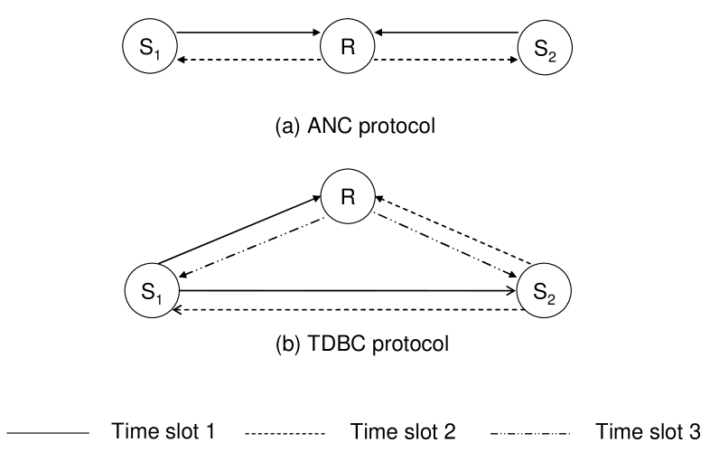
Figure 1: System models of the ANC and TDBC protocols.

The ANC protocol has received lots of attention recently [11], [12], and it is illustrated in Fig. 1(a). In this protocol, ${\mathrm{S}}_{1}$ and ${\mathrm{S}}_{2}$ simultaneously transmit to ${\mathrm{R}}$ at the first time slot with power $E$. Thus, the received signal $y_{R}(1)$ of ${\mathrm{R}}$ at the first time slot is given by

$$y_{R}(1)=\sqrt{E}hx_{1}+\sqrt{E}fx_{2}+n_{R}(1),$$ (1)

where $n_{R}(1)$ is the additive Gaussian noise. At the second time slot, ${\mathrm{R}}$ amplifies $y_{R}(1)$ with an amplifying coefficient $\rho$ and then transmits it to ${\mathrm{S}}_{1}$ and ${\mathrm{S}}_{2}$ also with power $E$. Consequently, the received signal $y_{S_{1}}(2)$ of ${\mathrm{S}}_{1}$ at the second time slot is given by

$$y_{S_{1}}(2) = \sqrt{E}\rho hy_{R}(1)+n_{S_{1}}(2)$$ (2)

$$= \rho h^{2}Ex_{1}+\rho hfEx_{2}+\rho h\sqrt{E}n_{R}(1)+n_{S_{1}}(2),$$ (3)

where $n_{S_{1}}(2)$ is the additive Gaussian noise. In order to ensure that the transmission power at ${\mathrm{R}}$ is always $E$, the amplifying coefficient is chosen as

$$\rho=\sqrt{\frac{1}{E|h|^{2}+E|f|^{2}+1}}.$$ (4)

Note that the received signal $y_{S_{1}}(2)$ contains both $x_{1}$ and $x_{2}$, where only $x_{2}$ is the desired signal and $x_{1}$ is actually an interference to ${\mathrm{S}}_{1}$. Since ${\mathrm{S}}_{1}$ perfectly knows $x_{1}$, it can completely remove $x_{1}$ from $y_{S_{1}}(2)$ and obtain a new signal $\tilde{y}_{S_{1}}(2)$ given by

$$\tilde{y}_{S_{1}}(2)=\rho hfEx_{2}+\rho h\sqrt{E}n_{R}(1)+n_{S_{1}}(2).$$ (5)

Consequently, the instantaneous SNR $\gamma_{1}^{{\mathrm{ANC}}}$ at ${\mathrm{S}}_{1}$ is given by

$$\gamma_{1}^{{\mathrm{ANC}}}=\frac{\rho^{2}|hf|^{2}E^{2}}{E\rho^{2}|h|^{2}+1}\approx\frac{E|hf|^{2}}{2|h|^{2}+|f|^{2}},$$ (6)

where the approximation is by letting $\rho\approx\sqrt{1/(E|h|^{2}+E|f|^{2})}$. Since this approximation is very tight in the whole SNR range, it has been used in many previous publications [21], [22]. Similarly, the instantaneous SNR $\gamma_{2}^{{\mathrm{ANC}}}$ at ${\mathrm{S}}_{2}$ is given by

$$\gamma_{2}^{{\mathrm{ANC}}}=\frac{\rho^{2}|hf|^{2}E^{2}}{E\rho^{2}|f|^{2}+1}\approx\frac{E|hf|^{2}}{2|f|^{2}+|h|^{2}}.$$ (7)

II-B Time Division Broadcast (TDBC)

In order to accomplish information exchange between ${\mathrm{S}}_{1}$ and ${\mathrm{S}}_{2}$, the TDBC protocol, as illustrated in Fig. 1(b), was studied in [13], [14]. As in the ANC protocol, we still assume that every terminal has the same transmission power $E$. At the first time slot, ${\mathrm{S}}_{1}$ transmits $x_{1}$ to ${\mathrm{R}}$ and ${\mathrm{S}}_{2}$. Thus, the received signals $y_{R}(1)$ of ${\mathrm{R}}$ and $y_{S_{2}}(1)$ of ${\mathrm{S}}_{2}$ at the first time slot are given by

$$y_{R}(1)=\sqrt{E}hx_{1}+n_{R}(1), y_{S_{2}}(1)=\sqrt{E}gx_{1}+n_{S_{2}}(1),$$ (8)

where $n_{R}(1)$ and $n_{S_{2}}(1)$ are the additive Gaussian noises. At the second time slot, ${\mathrm{S}}_{2}$ transmits $x_{2}$ to ${\mathrm{R}}$ and ${\mathrm{S}}_{1}$. The received signals $y_{R}(2)$ of ${\mathrm{R}}$ and $y_{S_{1}}(2)$ of ${\mathrm{S}}_{1}$ at the second time slot are given by

$$y_{R}(2)=\sqrt{E}fx_{2}+n_{R}(2), y_{S_{1}}(2)=\sqrt{E}gx_{2}+n_{S_{1}}(2),$$ (9)

where $n_{R}(2)$ and $n_{S_{1}}(2)$ are the additive Gaussian noises. At the third time slot, ${\mathrm{R}}$ combines $y_{R}(1)$ and $y_{R}(2)$ at first. Then it broadcasts the combined signal to ${\mathrm{S}}_{1}$ and ${\mathrm{S}}_{2}$. The combined signal at ${\mathrm{R}}$ is denoted by $x_{R}$ and it is given by

$$x_{R}=\eta_{1}y_{R}(1)+\eta_{2}y_{R}(2),$$ (10)

where

$$\eta_{1}=\sqrt{\frac{\xi}{E|h|^{2}+1}}, \eta_{2}=\sqrt{\frac{(1-\xi)}{E|f|^{2}+1}}.$$ (11)

The choice of $\eta_{1}$ and $\eta_{2}$ ensures that $x_{R}$ always has unit power. The value of $\xi$ decides how the relay combines the signals received from two different sources and it can be used to optimize the performance of the TDBC protocol, which will be discussed in detail later.

At the third time slot, the received signal $y_{S_{1}}(3)$ of ${\mathrm{S}}_{1}$ is given by

$$y_{S_{1}}(3) = \sqrt{E}hx_{R}+n_{S_{1}}(3)$$ (12)

$$= \eta_{1}h^{2}Ex_{1}+\eta_{2}hfEx_{2}+\eta_{1}h\sqrt{E}n_{R}(1)+\eta_{2}h\sqrt{E}n_{R}(2)+n_{S_{1}}(3).$$ (13)

As in the ANC protocol, ${\mathrm{S}}_{1}$ can completely remove $x_{1}$ and obtain a new signal $\tilde{y}_{S_{1}}(3)$ given by

$$\tilde{y}_{S_{1}}(3)=\eta_{2}hfEx_{2}+\eta_{1}h\sqrt{E}n_{R}(1)+\eta_{2}h\sqrt{E}n_{R}(2)+n_{S_{1}}(3).$$ (14)

Then ${\mathrm{S}}_{1}$ combines $\tilde{y}_{S_{1}}(3)$ with $y_{S_{1}}(2)$ by maximum ratio combining and the instantaneous SNR $\gamma_{1}^{{\mathrm{TDBC}}}$ of the combined signal is

$$\gamma_{1}^{{\mathrm{TDBC}}}=E|g|^{2}+\frac{E^{2}\eta_{2}^{2}|hf|^{2}}{E|h|^{2}(\eta_{1}^{2}+\eta_{2}^{2})+1}\approx E|g|^{2}+\frac{(1-\xi)E|hf|^{2}}{|f|^{2}(\xi+1)+(1-\xi)|h|^{2}},$$ (15)

where the approximation is due to $\eta_{1}\approx\sqrt{\xi/(E|h|^{2})}$ and $\eta_{2}\approx\sqrt{(1-\xi)/(E|f|^{2})}$. Similarly, the instantaneous SNR $\gamma_{2}^{{\mathrm{TDBC}}}$ at ${\mathrm{S}}_{2}$ is

$$\gamma_{2}^{{\mathrm{TDBC}}}=E|g|^{2}+\frac{E^{2}\eta_{1}^{2}|hf|^{2}}{E|f|^{2}(\eta_{1}^{2}+\eta_{2}^{2})+1} \approx E|g|^{2}+\frac{\xi E|hf|^{2}}{|h|^{2}(2-\xi)+\xi|f|^{2}}.$$ (16)

III Outage Probability and Finite-SNR Diversity-Multiplexing Tradeoff

In this section, we derive lower bounds of the outage probabilities of the ANC and TDBC protocols. They are very tight in the whole SNR range, irrespective of the values of channel variances. Furthermore, based on those lower bounds, we derive the finite-SNR diversity-multiplexing tradeoffs of the ANC and TDBC protocols.

III-A Analog Network Coding

When the ANC protocol is used, it follows from (6) and (7) that the mutual information at ${\mathrm{S}}_{1}$ and ${\mathrm{S}}_{2}$ is given by

$$I_{1}^{\mathrm{ANC}}=\frac{1}{2}\log\left(1+\gamma_{1}^{{\mathrm{ANC}}}\right), I_{2}^{\mathrm{ANC}}=\frac{1}{2}\log\left(1+\gamma_{2}^{{\mathrm{ANC}}}\right).$$ (17)

Note that the pre-log factor $1/2$ is because the information exchange between the two sources takes two time slots [7]. Assume that the target rate of the whole bidirectional cooperative network is $R$. Since the two sources in this network are equivalent terminals, it is fair to set the target rate of each source as $R/2$. Furthermore, in a bidirectional cooperative network, the two sources are not only transmitters but also receivers. Due to this reason, a bidirectional cooperative network can be seen as a multiuser system. It is well known that a multiuser system is in outage when any user is in outage [27], [28]. Therefore, the ANC protocol is in outage when either $I_{1}^{{\mathrm{ANC}}}$ or $I_{2}^{\mathrm{ANC}}$ is smaller than the target rate $R/2$, i.e.

$$P_{{\mathrm{ANC}}}^{{\mathrm{outage}}}(R)=\Pr\left(I_{1}^{\mathrm{ANC}}<\frac{R}{2}\ \ {\mathrm{or}}\ \ I_{2}^{\mathrm{ANC}}<\frac{R}{2}\right).$$ (18)

The exact expression of the outage probability is very hard to derive even after we approximate the instantaneous SNRs as in (6) and (7). However, it is well known that the harmonic mean of two positive numbers can be upper-bounded by the minimum of those two numbers as follows [21]:

$$\frac{xy}{x+y}<\min(x,y).$$ (19)

In order to make the analysis feasible, we use this method to upper-bound the instantaneous SNRs and derive a lower bound of the outage probability in the following lemma.

Lemma 1

The outage probability of the ANC protocol can be lower-bounded as follows:

$$P_{{\mathrm{ANC}}}^{{\mathrm{outage}}}(R)>\tilde{P}_{{\mathrm{ANC}}}^{{\mathrm{outage}}}(R)=1-\exp\left(-\frac{2\left(\Omega_{h}+\Omega_{f}\right)\left(2^{R}-1\right)}{E\Omega_{h}\Omega_{f}}\right).$$ (20)

Proof:

See Appendix A. ∎

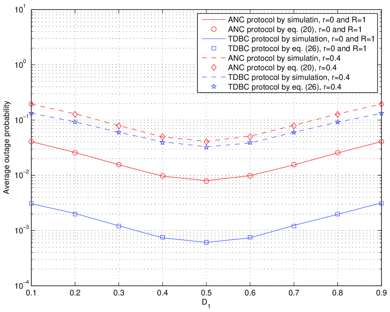
Figure 4: Outage probabilities of the ANC and TDBC protocols with equal power allocation and $\xi=1/2$, $10\log_{10}E=15$ dB.

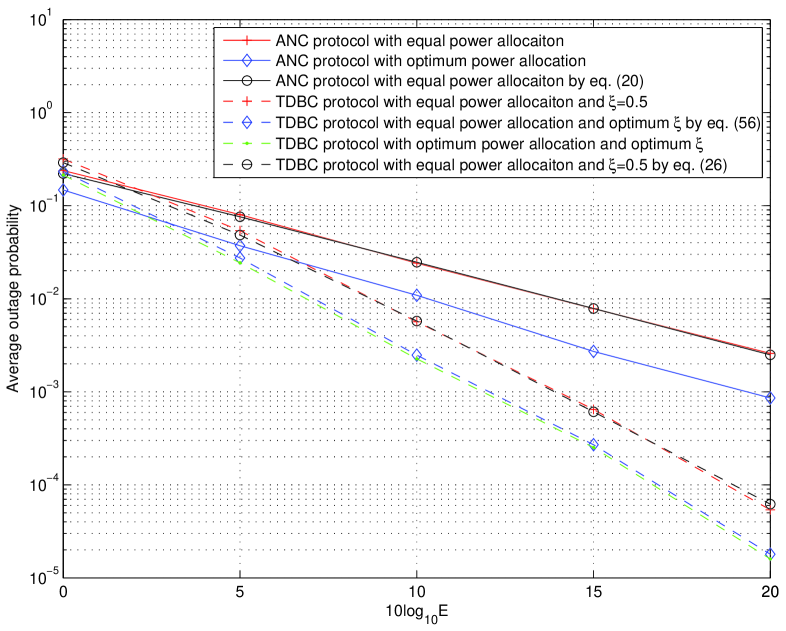
Figure 5: Outage probabilities of the ANC and TDBC protocols, $D_{1}=0.5$, $r=0$, and $R=1$ bps/Hz.

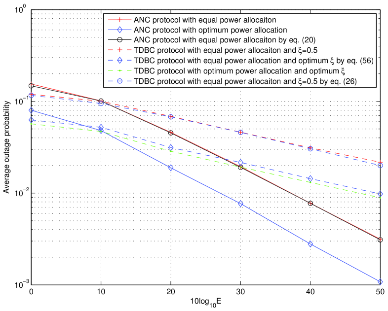
Figure 6: Outage probabilities of the ANC and TDBC protocols, $D_{1}=0.4$ and $r=0.6$.

We notice that, irrespective of the values of channel variances, the lower bound $\tilde{P}_{\mathrm{ANC}}^{\mathrm{outage}}(R)$ is extremely tight in the whole SNR range as shown in Figs. 4–6. Due to this reason, we use this lower bound to find the finite-SNR diversity-multiplexing tradeoff of the ANC protocol as in [24] and it is given in the follow theorem.

Theorem 1

The finite-SNR diversity-multiplexing tradeoff curve $d^{\mathrm{ANC}}(r,E)$ of the ANC protocol is given by

$$d^{\mathrm{ANC}}(r,E)=\frac{2(\Omega_{h}+\Omega_{f})\left(1+rE(1+E)^{r-1}-(1+E)^{r}\right)}{E\Omega_{h}\Omega_{f}\left(1-\exp\left(\frac{2(\Omega_{h}+\Omega_{f})}{E\Omega_{h}\Omega_{f}}\left((1+E)^{r}-1\right)\right)\right)}, 0\leq r\leq 1.$$ (21)

Proof:

By definition, the finite-SNR diversity-multiplexing tradeoff curve $d^{\mathrm{ANC}}(r,E)$ is given by [24]

$$d^{\mathrm{ANC}}(r,E)=-\frac{\partial\ln\tilde{P}^{\mathrm{outage}}_{\mathrm{ANC}}(r\log(1+aE))}{\partial\ln E},$$ (22)

where $a$ is a constant and called array gain. Since every terminal has only one antenna, we set $a=1$ according to its definition in [24]. By substituting (20) into (22), one can easily obtain (21). ∎

An interesting special case of the trade-off curve $d^{\mathrm{ANC}}(r,E)$ is when the SNR goes to infinity. This actually corresponds to the definition of infinite-SNR diversity-multiplexing tradeoff given in [20]. For this case, the tradeoff curve of the ANC protocol becomes

$$\lim_{E\rightarrow\infty}d^{\mathrm{ANC}}(r,E)=1-r,\ \ \ \ 0\leq r\leq 1.$$ (23)

Based on (23), we see that the maximum multiplexing gain of the ANC protocol is one. This is because, although each traffic flow in the ANC protocol takes two time slots to complete the transmission, there are two concurrent traffic flows and they are supported by the same physical channels. Note that, in a conventional unidirectional cooperative network, there is only one traffic flow in the network, and hence, the maximum multiplexing gain of such network is just $1/2$. As a result, the ANC protocol indeed has much higher bandwidth efficiency than the conventional unidirectional cooperative networks. However, the maximum diversity gain of the ANC protocol is just one. This is because the ANC protocol let the two sources transmit simultaneously at the first time slot. As a result, the sources can not receive the signals from the direct channel due to the half-duplex constraint. In order to achieve higher diversity gain, we can assign one time slot to each source and let them transmit separately as in the TDBC protocol discussed in the next subsection. As we will show, however, this leads to some loss of multiplexing gain.

III-B Time Division Broadcasting

When a bidirectional cooperative network implements the TDBC protocol, the mutual information at ${\mathrm{S}}_{1}$ and ${\mathrm{S}}_{2}$ is given by

$$I_{1}^{\mathrm{TDBC}}=\frac{1}{3}\log\left(1+\gamma_{1}^{\mathrm{TDBC}}\right), I_{2}^{\mathrm{TDBC}}=\frac{1}{3}\log\left(1+\gamma_{2}^{\mathrm{TDBC}}\right),$$ (24)

where the instantaneous SNRs are given by (15) and (16), respectively. The pre-log factor $1/3$ is because each traffic flow takes three time slots in the TDBC protocol. As for the ANC protocol, the TDBC protocol is in outage when either $I_{1}^{\mathrm{TDBC}}$ or $I_{2}^{\mathrm{TDBC}}$ is smaller than the target rate $R/2$, i.e.

$$P_{{\mathrm{TDBC}}}^{{\mathrm{outage}}}(R)=\Pr\left(I_{1}^{\mathrm{TDBC}}<\frac{R}{2}\ \ {\mathrm{or}}\ \ I_{2}^{\mathrm{TDBC}}<\frac{R}{2}\right).$$ (25)

It is very hard to obtain the exact expression of $P_{{\mathrm{TDBC}}}^{{\mathrm{outage}}}(R)$ even after using the approximations in (15) and (16). In order to make the problem tractable, we still use (19) to upper-bound the instantaneous SNRs. Furthermore, we let $\xi=1/2$ to simplify the derivation in this subsection. This actually means that ${\mathrm{R}}$ uses half of its power to transmit to ${\mathrm{S}}_{1}$ and uses the other half to ${\mathrm{S}}_{2}$. In Subsection IV-B, we will consider how ${\mathrm{R}}$ can optimally allocate its transmission power for ${\mathrm{S}}_{1}$ and ${\mathrm{S}}_{2}$ by choosing an optimum value of $\xi$. A lower bound of the outage probability of the TDBC protocol is given in the following lemma.

Lemma 2

When $\xi=1/2$, the outage probability $P_{\mathrm{TDBC}}^{\mathrm{outage}}(R)$ of the TDBC protocol can be lower-bounded as follows:

$$P_{\mathrm{TDBC}}^{\mathrm{outage}}(R)>\tilde{P}_{\mathrm{TDBC}}^{\mathrm{outage}}(R) = 1-\frac{1}{3\Omega_{f}\Omega_{g}+3\Omega_{h}\Omega_{g}-\Omega_{h}\Omega_{f}}$$ (26)

$$\times\left(3\Omega_{g}\left(\Omega_{f}+\Omega_{h}\right)\exp\left(-\frac{2^{1.5R}-1}{E\Omega_{g}}\right)\right.$$

$$\left.-\Omega_{h}\Omega_{f}\exp\left(-\frac{3(2^{1.5R}-1)(\Omega_{h}+\Omega_{f})}{E\Omega_{h}\Omega_{f}}\right)\right).$$

Proof:

See Appendix B. ∎

Figs. 4–6 demonstrate that this lower bound $\tilde{P}_{\mathrm{TDBC}}^{\mathrm{outage}}(R)$ is extremely tight in the whole SNR range, irrespective of the values of channel variances. Therefore, we use this lower bound to find the finite-SNR diversity-multiplexing tradeoff of the TDBC protocol and it is given in the follow theorem.

Theorem 2

The finite-SNR diversity-multiplexing tradeoff curve $d^{\mathrm{TDBC}}(r,E)$ of the TDBC protocol is given by

$$d^{\mathrm{TDBC}}(r,E)=\frac{d_{1}(r,E)}{d_{2}(r,E)}, 0\leq r\leq\frac{2}{3},$$ (27)

where

$$d_{1}(r,E) = 3(\Omega_{h}+\Omega_{f})(\lambda(3rE-2E-2)+2E+2)$$ (28)

$$\times\left(\exp\left(-\frac{3(\Omega_{h}+\Omega_{f})}{E\Omega_{h}\Omega_{f}}(\lambda-1)\right)-\exp\left(-\frac{\lambda-1}{E\Omega_{g}}\right)\right),$$

$$d_{2}(r,E) = 2E(E+1)\left(3\Omega_{g}(\Omega_{h}+\Omega_{f})\left(1-\exp\left(-\frac{\lambda-1}{E\Omega_{g}}\right)\right)\right.$$ (29)

$$\left.-\Omega_{h}\Omega_{f}\left(1-\exp\left(-\frac{3(\Omega_{h}+\Omega_{f})}{E\Omega_{h}\Omega_{f}}(\lambda-1)\right)\right)\right),$$

$$\lambda = (1+E)^{\frac{3r}{2}}.$$ (30)

Proof:

The proof is essentially the same as that of Theorem 1, except that we use the lower bound $\tilde{P}_{\mathrm{TDBC}}^{\mathrm{outage}}(R)$ of the TDBC protocol instead of $\tilde{P}_{\mathrm{ANC}}^{\mathrm{outage}}(R)$. ∎

When the SNR goes to infinity, the trade-off curve $d^{\mathrm{TDBC}}(r,E)$ becomes

$$\lim_{E\rightarrow\infty}d^{\mathrm{TDBC}}(r,E)=2-3r, 0\leq r\leq\frac{2}{3}.$$ (31)

As a result, the maximum multiplexing gain of the TDBC protocol is $2/3$, which is smaller than that of the ANC protocol. This is because, although the TDBC protocol supports two traffic flows concurrently as the ANC protocol, each traffic flow takes three time slots to complete the transmission as opposed to two time slots in the ANC protocol. Due to this reason, the bandwidth efficiency of the TDBC protocol is not as high as that of the ANC protocol. However, note that the maximum multiplexing gain of the TDBC protocol is still larger than that of the conventional unidirectional cooperative networks. On the other hand, the maximum diversity gain of the TDBC protocol is indeed two as shown in [13], [14], and it is much larger than that of the ANC protocol. Moreover, based on (23) and (31), those two protocols achieve the same diversity gain at $r=1/2$ when SNR goes to infinity.

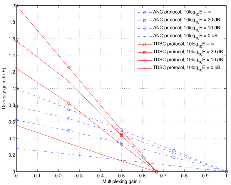
Figure 2: Diversity-multiplexing tradeoffs of the ANC and TDBC protocols, $D_{1}=0.5$.

Many previous publications on bidirectional cooperative networks did not consider the direct channel between the two sources [8], [11], [12], and [15]–[18]. As a result, the maximum diversity gain of the TDBC protocol is just one which is the same as that of the ANC protocol. Since the maximum multiplexing gain of the TDBC protocol is never larger than that of the ANC protocol, the ANC protocol always outperforms the TDBC protocol in terms of diversity-multiplexing tradeoff. When the direct channel exists, however, the ANC protocol no longer outperforms the TDBC protocol for all the time. As shown in Fig. 2, those two protocols achieve the same diversity gain when the multiplexing gain is approximately $1/2$. When the multiplexing gain becomes smaller, the TDBC protocol outperforms the ANC protocol as it achieves a higher diversity gain; while, when the multiplexing gain becomes bigger, the ANC protocol outperforms. This implies that the ANC protocol can transmit information more efficiently, but the TDBC protocol can transmit information more reliably. Therefore, one may alternatively use those two protocols depending on the specific task of a bidirectional cooperative network.

Certainly, it is desirable to find when the ANC and TDBC protocols have the same diversity gain for a fixed $E$ by solving the equation $d^{\mathrm{ANC}}(r,E)=d^{\mathrm{TDBC}}(r,E)$. Let $Q(E)$ denote the solution to this equation. However, the exact expression of $Q(E)$ can not be given in closed form. In the following corollary, we present a very accurate approximation to $Q(E)$.

Corollary 1

When $E$ is fixed, the solution $Q(E)$ to the equation $d^{\mathrm{ANC}}(r,E)=d^{\mathrm{TDBC}}(r,E)$ can be approximated by

$$Q(E)\approx\tilde{Q}(E)=\frac{1}{2}-\frac{\nu_{1}-\mu_{1}}{\nu_{2}-\mu_{2}}.$$ (32)

The coefficients $\mu_{1}$, $\mu_{2}$, $\nu_{1}$, and $\nu_{2}$ are given as follows:

$$\mu_{1} = \frac{2\left(\Omega_{h}+\Omega_{f}\right)\left(\,{\frac{E}{2\sqrt{1+E}}}+1-\sqrt{1+E}\right)}{{E}{\Omega_{h}}{\Omega_{f}}\left(1-c_{1}\right)},$$ (33)

$$\mu_{2} = \frac{2(\Omega_{h}+\Omega_{f})}{E\Omega_{h}\Omega_{f}(1-c_{1})}\left(\frac{E\ln(1+E)+2E}{2\sqrt{1+E}}-\sqrt{1+E}\ln(1+E)\right.$$ (35)

$$\left.+\frac{c_{1}(\Omega_{h}+\Omega_{f})(E-2\sqrt{1+E}+2)\ln(1+E)}{E\Omega_{h}\Omega_{f}(c_{1}-1)}\right),$$

$$\nu_{1} = \frac{3(c_{3}-c_{2})(\Omega_{h}+\Omega_{f})\left(4(1+E)^{\frac{1}{4}}-E-4\right)}{E(1+E)^{\frac{1}{4}}(3\Omega_{g}(\Omega_{h}+\Omega_{f})(1-c_{2})-\Omega_{h}\Omega_{f}(1-c_{3}))},$$ (36)

$$\nu_{2} = \frac{3(\Omega_{h}+\Omega_{f})}{E(1+E)^{\frac{1}{4}}}\left((c_{3}-c_{2})\left(E-\frac{1}{4}(E+4)\ln(1+E)\right)\right.$$ (37)

$$\left.+\frac{\ln(1+E)}{2E}\left(\frac{c_{2}}{\Omega_{g}}-\frac{3c_{3}(\Omega_{h}+\Omega_{f})}{\Omega_{h}\Omega_{f}}\right)(1+E)^{\frac{3}{4}}\left(2(1+E)^{\frac{1}{4}}-\frac{E}{2}-2\right)\right)$$

$$+\frac{9(c_{2}-c_{3})^{2}(\Omega_{h}+\Omega_{f})^{2}\left(E+4-4(1+E)^{\frac{1}{4}}\right)(1+E)^{\frac{3}{4}}\ln(1+E)}{4E^{2}(1+E)^{\frac{1}{4}}(3\Omega_{g}(\Omega_{h}+\Omega_{f})(c_{2}-1)+\Omega_{h}\Omega_{f}(1-c_{3}))},$$

where $c_{1}$, $c_{2}$, $c_{3}$ are constants and they are given by

$$c_{1} = \exp\left(\frac{2\left(\Omega_{h}+\Omega_{f}\right)\left(\sqrt{1+E}-1\right)}{E\Omega_{h}\Omega_{f}}\right)$$ (38)

$$c_{2} = \exp\left(\frac{1-(1+E)^{\frac{3}{4}}}{E\Omega_{g}}\right)$$ (39)

$$c_{3} = \exp\left(\frac{3(\Omega_{h}+\Omega_{f})(1-(1+E)^{\frac{3}{4}})}{E\Omega_{g}}\right).$$ (40)

Proof:

In Fig. 2, we notice that both $d^{\mathrm{ANC}}(r,E)$ and $d^{\mathrm{TDBC}}(r,E)$ can be accurately approximated by linear functions. Furthermore, the solution $Q(E)$ to this equation $d^{\mathrm{ANC}}(r,E)=d^{\mathrm{TDBC}}(r,E)$ is very close to $r=1/2$, irrespective of the value of $E$. Therefore, we approximate $d^{\mathrm{ANC}}(r,E)$ and $d^{\mathrm{TDBC}}(r,E)$ by Taylor expansion as follows:

$$d^{\mathrm{ANC}}(r,E)\approx\mu_{1}+\mu_{2}\left(r-\frac{1}{2}\right), d^{\mathrm{TDBC}}(r,E)\approx\nu_{1}+\nu_{2}\left(r-\frac{1}{2}\right),$$ (41)

where the coefficients $\mu_{1}$, $\mu_{2}$, $\nu_{1}$, and $\nu_{2}$ are given in (33)–(37). By using (41), one can easily obtain $\tilde{Q}(E)$. ∎

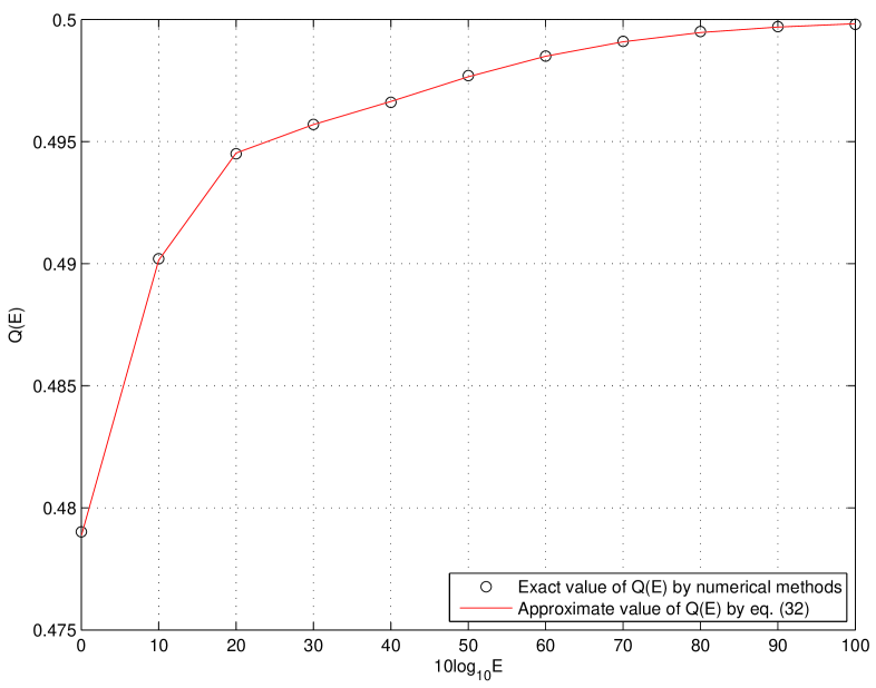
Figure 3: Values of $Q(E)$, $D_{1}=0.5$.

Fig. 3 demonstrates that $\tilde{Q}(E)$ is a very tight approximation of $Q(E)$. When the SNR goes to infinity, we can show that

$$\lim_{E\rightarrow\infty}\tilde{Q}(E)=\frac{1}{2}.$$ (42)

This coincides with our conclusion based on (23) and (31). Furthermore, it is not hard to analytically show that $\tilde{Q}(E)$ is always smaller than or equal to $1/2$ for any $E$, which implies that the ANC protocol achieves a higher diversity gain than the TDBC protocol as long as the multiplexing gain is lager than $1/2$.

Note that our outage probability lower bounds and finite-SNR diversity-multiplexing tradeoffs of the ANC and TDBC protocols are based on the assumption that there is a direct channel between the two sources. When such direct channel does not exist as in [8], [11], [12], and [15]–[19], however, out results can be easily extended to this special case by letting $\Omega_{g}=0$. For the ANC protocol, the lower bound $\tilde{P}_{\mathrm{ANC}}^{\mathrm{outage}}(R)$ and diversity-multiplexing tradeoff $d^{\mathrm{ANC}}(r,E)$ do not change. For the TDBC protocol, the lower bound of the outage probability and the diversity-multiplexing tradeoff now become

$$\tilde{P}_{\mathrm{TDBC}}^{\mathrm{outage}}(R) = 1-\exp\left(-\frac{3(2^{1.5R}-1)(\Omega_{h}+\Omega_{f})}{E\Omega_{h}\Omega_{f}}\right),$$ (43)

$$d^{\mathrm{TDBC}}(r,E)=\frac{3(\Omega_{h}+\Omega_{f})(\lambda(3rE-2E-2)+2E+2)\exp\left(-\frac{3(\Omega_{h}+\Omega_{f})}{E\Omega_{h}\Omega_{f}}(\lambda-1)\right)}{2E(E+1)\Omega_{h}\Omega_{f}\left(\exp\left(-\frac{3(\Omega_{h}+\Omega_{f})}{E\Omega_{h}\Omega_{f}}(\lambda-1)\right)-1\right)}.$$ (44)

Furthermore, when the SNR goes to infinity, the trade-off curve of the TDBC protocol becomes

$$\lim_{E\rightarrow\infty}d^{\mathrm{TDBC}}(r,E)=1-\frac{3}{2}r, 0\leq r\leq\frac{2}{3}.$$ (45)

By comparing (45) and (23), one can see that the ANC protocol indeed always outperforms the TDBC protocol in terms of diversity-multiplexing tradeoff when the direct channel does not exist. This coincides with the conclusion which can be drawn from [8], [11], and [19].

IV Optimum Power Allocation

In this section, we first propose an optimum power allocation scheme for the ANC protocol. This scheme can simultaneously minimize the outage probability and maximize the total mutual information of the ANC protocol. Secondly, we develop an optimum method for the TDBC protocol to combine the received signals at the relay. This method also minimizes the outage probability and maximizes the total mutual information of the TDBC protocol at the same time.

IV-A Analog Network Coding

In Subsection III-A, we derive a lower bound of the outage probability of the ANC protocol when every terminal has the same transmission power $E$. Since every terminal knows the values of $h$ and $f$, it is more desirable to allocate the transmission power according to channel conditions in order to maximize the performance. Such power allocation problem has not been investigated yet in previous publications. We now assume that the transmission powers of ${\mathrm{S}}_{1}$, ${\mathrm{S}}_{2}$, and ${\mathrm{R}}$ are $E_{1}$, $E_{2}$, and $E_{r}$, respectively. Consequently, the instantaneous SNRs at ${\mathrm{S}}_{1}$ and ${\mathrm{S}}_{2}$ should be rewritten as

$$\gamma_{1}^{{\mathrm{ANC}}}\approx\frac{E_{r}E_{2}|hf|^{2}}{(E_{r}+E_{1})|h|^{2}+E_{2}|f|^{2}}, \gamma_{2}^{{\mathrm{ANC}}}\approx\frac{E_{r}E_{1}|hf|^{2}}{(E_{r}+E_{2})|f|^{2}+E_{1}|h|^{2}}.$$ (46)

When it comes to optimum power allocation, two optimization goals are usually considered: minimization of the outage probability and maximization of the total mutual information. We first use the outage probability as the metric to optimally allocate the power. That is, the optimization problem is formulated by

$$(E_{1},E_{2},E_{r})=\arg\min_{E_{1},E_{2},E_{r}}P_{\mathrm{ANC}}^{\mathrm{outage}}(R), {\mathrm{subject\ to}}\ \ \ E_{1}+E_{2}+E_{r}=3E.$$ (47)

It follows from (18) that the optimization problem in (47) is equivalent to the following one

$$(E_{1},E_{2},E_{r})=\arg\max_{E_{1},E_{2},E_{r}}\min(\gamma_{1}^{\mathrm{ANC}},\gamma_{2}^{\mathrm{ANC}}), {\mathrm{subject\ to}}\ \ \ E_{1}+E_{2}+E_{r}=3E.$$ (48)

The minimax problem in (48) is solved in the following theorem.

Theorem 3

When $E_{1}+E_{2}+E_{r}=3E$, the optimum power allocation that minimizes the outage probability $P_{\mathrm{ANC}}^{\mathrm{outage}}(R)$ of the ANC protocol is given by

$$E_{r} = \frac{3}{2}E,$$ (49)

$$E_{1} = \frac{3|f|}{2(|h|+|f|)}E,$$ (50)

$$E_{2} = \frac{3|h|}{2(|h|+|f|)}E.$$ (51)

Proof:

See Appendix C. ∎

Secondly, we consider the optimum power allocation scheme that maximizes the total mutual information $I^{\mathrm{ANC}}=I_{1}^{\mathrm{ANC}}+I_{2}^{\mathrm{ANC}}$ of the ANC protocol. Therefore, the optimization problem is formulated as

$$(E_{1},E_{2},E_{r})=\arg\max_{E_{1},E_{2},E_{r}}I^{\mathrm{ANC}}, {\mathrm{subject\ to}}\ \ \ E_{1}+E_{2}+E_{r}=3E.$$ (52)

This optimization problem is solved in the following lemma.

Lemma 3

When $E_{1}+E_{2}+E_{r}=3E$, the optimum power allocation scheme that maximizes the total mutual information $I^{\mathrm{ANC}}$ of the ANC protocol is given by (49)–(51).

Proof:

Let $E_{1}=3\alpha E$, $E_{2}=3\beta E$, and $E_{r}=3(1-\alpha-\beta)E$, where $0\leq\alpha\leq 1$, $0\leq\beta\leq 1$, and $\alpha+\beta\leq 1$. With those constraints, the solution to $\partial I^{\mathrm{ANC}}/\partial\alpha=0$ and $\partial I^{\mathrm{ANC}}/\partial\beta=0$ is given by

$$\alpha=\frac{|f|}{2(|h|+|f|)}, \beta=\frac{|h|}{2(|h|+|f|)}.$$ (53)

As a result, the optimum power allocation scheme is given by (49)–(51). ∎

Interestingly, the optimum power allocation schemes based on outage probability and total mutual information are exactly the same. This is due to the special structures of the instantaneous SNRs $\gamma_{1}^{\mathrm{ANC}}$ and $\gamma_{2}^{\mathrm{ANC}}$ given in (46). As a result, we obtain an optimum power allocation scheme that simultaneously minimizes the outage probability and maximizes the total mutual information of the ANC protocol.

IV-B Time Division Broadcasting

Unlike the ANC protocol, it is very hard to find an optimum power allocation scheme for the TDBC protocol no matter using the outage probability or the total mutual information as the criteria. For example, if we intend to minimize the outage probability, the optimization problem is a generalized fractional programming problem. Such problem can only be solved numerically for most cases [31], [32]. However, the optimum value of $\xi$ can be analytically found in closed form and it can greatly improve the performance. We first try to find the optimum value of $\xi$ that minimizes the outage probability of the TDBC protocol. That is, we consider the following optimization problem

$$\xi=\arg\min_{\xi}P_{\mathrm{TDBC}}^{\mathrm{outage}}(R), {\mathrm{subject\ to}}\ \ \ 0\leq\xi\leq 1.$$ (54)

It follows from (25) that the optimization problem in (54) is equivalent to the following one

$$\xi=\arg\mathop{\max}_{\xi}\min(\gamma_{1}^{\mathrm{TDBC}},\gamma_{2}^{\mathrm{TDBC}}), {\mathrm{subject\ to}}\ \ \ 0\leq\xi\leq 1.$$ (55)

The solution to (55) is given in a simple and closed form in the following theorem.

Theorem 4

The optimum value of $\xi$ that minimizes the outage probability $P_{\mathrm{TDBC}}^{\mathrm{outage}}(R)$ of the TDBC protocol is given by

$$\xi=\frac{|h|}{|h|+|f|}.$$ (56)

Proof:

See Appendix D. ∎

Note that the optimum value of $\xi$ given in Theorem 4 is based on the assumption that every terminal has the same transmission power $E$. Certainly, one can jointly optimize the value of $\xi$ and the transmission power of every terminal to minimize the outage probability, but this can only be done numerically. Actually, by letting every terminal has the same transmission power $E$ and letting $\xi$ equal to $|h|/(|h|+|f|)$ as in (56), the performance of the network is almost the same as that of the network where the transmission powers and the value of $\xi$ are jointly optimized by numerical ways as shown in Figs. 5 and 6.

Secondly, we investigate the optimum value of $\xi$ that maximizes the total mutual information $I^{\mathrm{TDBC}}=I_{1}^{\mathrm{TDBC}}+I_{2}^{\mathrm{TDBC}}$ of the TDBC protocol, i.e.

$$\xi=\arg\max_{\xi}I^{\mathrm{TDBC}}, {\mathrm{subject\ to}}\ \ 0\leq\xi\leq 1,$$ (57)

where $I_{1}^{\mathrm{TDBC}}$ and $I_{2}^{\mathrm{TDBC}}$ are given by (24). The solution to (57) is given the following lemma.

Lemma 4

The optimum value of $\xi$ that maximizes the total mutual information $I^{\mathrm{TDBC}}$ of the TDBC protocol is given by (56).

Proof:

By solving the equation $\partial I^{\mathrm{TDBC}}/\partial\xi=0$, we can easily obtained the solution given in (56). ∎

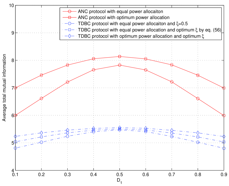
Figure 7: Total mutual information of the ANC and TDBC protocols, $10\log_{10}E=20$ dB.

As for Theorem 4, the optimum value of $\xi$ in Lemma 4 is also based on the setting that every terminal has the same transmission power $E$. The joint optimization of the transmission powers and the value of $\xi$ to maximize the total mutual information can only be accomplished by numerical ways. In fact, by simply letting every terminal has the same transmission power $E$ and letting $\xi$ equal to (56), the total mutual information of the TDBC protocol can be improved substantially as shown in Fig. 7.

Interestingly, we notice that the optimum values of $\xi$ in Theorem 4 and Lemma 4 are exactly the same, although they are based on two different criteria. As a result, by letting $\xi$ equal to $|h|/(|h|+|f|)$, we can minimize the outage probability and maximize the total mutual information of the TDBC protocol at the same time. Actually, the reason why we can find such $\xi$ is because every terminal has the same transmission power. In general, when every terminal has unequal transmission power, the solutions to (55) and (57) are different. Furthermore, the joint optimization of the transmission powers and the value of $\xi$ based on the outage probability criteria is also generally different with that based on the total mutual information criteria. Thus, one may use equal power allocation and set $\xi$ as (56) in order to transmit information efficiently and reliably at the same time.

V Numerical Results

In this section, we present some numerical results to demonstrate the performance of the ANC and TDBC protocols. We assume that all three terminals are located in a straight line and ${\mathrm{R}}$ is between ${\mathrm{S}}_{1}$ and ${\mathrm{S}}_{2}$. We fix the distance between ${\mathrm{S}}_{1}$ and ${\mathrm{S}}_{2}$ as one and let $D_{1}$ denote the distance between ${\mathrm{S}}_{1}$ and ${\mathrm{S}}_{2}$. Furthermore, we set the path loss factor as four in order to model radio propagation in urban areas [33]. As a result, the values of $\Omega_{g}$, $\Omega_{h}$ and $\Omega_{f}$ equal to one, $D_{1}^{-4}$, and $(1-D_{1})^{-4}$, respectively.

In Fig. 2, we compare the diversity-multiplexing tradeoffs of the ANC and TDBC protocols. For each protocol, its finite-SNR diversity-multiplexing tradeoff indeed converges to the infinite-SNR case when $E$ goes to infinity. When $E$ is fixed, the tradeoff curves of those two protocols have a cross point at approximately $r=1/2$ as expected by Corollary 1. Fig. 3 shows the values of $Q(E)$, and hence, it demonstrates when the ANC and TDBC protocols have the same diversity gain. One can see that our approximate solution $\tilde{Q}(E)$ is extremely tight to the exact one $Q(E)$ which is obtained by a numerical method.

In Fig. 4, we compare the exact outage probabilities of the ANC and TDBC protocols with our lower bounds given in (20) and (26). It can be seen that the lower bounds are extremely tight for both protocols even when we change the location of the relay and the value of multiplexing gain. Furthermore, in Figs. 5 and 6, we see that our lower bounds are constantly tight in the whole SNR range. In Fig. 5, we let the multiplexing gain equal to zero. As a result, the TDBC protocol achieves a higher diversity gain than the ANC protocol, which coincides with our conclusion drawn from Fig. 2. On the other hand, we let the multiplexing gain equal to $0.6$ in Fig. 6 and show that the ANC protocol has a higher diversity gain for this case.

In Figs. 5 and 6, one can also see that the optimum power allocation scheme of the ANC protocol substantially reduces the outage probability even when the relay is exactly in the middle of the two sources. For the TDBC protocol, its outage probability is considerably reduced as well when the proposed combing method given in (56) is implemented with equal power allocation. Moreover, by letting $\xi$ equal to (56) and adopting equal power allocation, we can achieve almost the same outage probability as jointly optimizing the value of $\xi$ and the transmission powers by numerical ways.

In Fig. 7, we show that the optimum power allocation scheme can considerably increase the total mutual information of the ANC protocol especially when ${\mathrm{R}}$ is close to either ${\mathrm{S}}_{1}$ or ${\mathrm{S}}_{2}$. Moreover, the proposed optimum combing method with equal power allocation can greatly increase the total mutual information of the TDBC protocol as well, but the improvement is not as considerable as that achieved by joint optimization of $\xi$ and the transmission powers.

VI Conclusion

This paper studies the ANC and TDBC protocols which are used to achieve information exchange in bidirectional cooperative networks. We derive lower bounds of the outage probabilities of those two protocols. The lower bounds are extremely tight in the whole SNR range irrespective of the values of channel variances. Therefore, based on those lower bounds, we derive the finite-SNR diversity-multiplexing tradeoffs of the ANC and TDBC protocols. Furthermore, we propose an optimum power allocation scheme for the ANC protocol. This scheme can simultaneously minimize the outage probability and maximize the total mutual information of the ANC protocol. For the TDBC protocol, we develop an optimum combing method for the relay terminal under an equal power allocation assumption. This method substantially reduces the outage probability and increases the total mutual information as well.

Appendix A

Proof of Lemma 1

Let $X=|h|^{2}$ and $Y=|f|^{2}$. Thus, $X$ and $Y$ are exponential random variables with means $\Omega_{h}$ and $\Omega_{f}$, respectively. By using the inequality (19), the outage probability can be lower-bounded as follows:

$$P_{{\mathrm{ANC}}}^{{\mathrm{outage}}}(R) = \Pr\left(I_{1}^{\mathrm{ANC}}<\frac{R}{2}\ \ {\mathrm{or}}\ \ I_{2}^{\mathrm{ANC}}<\frac{R}{2}\right)$$ (A.1)

$$= 1-\Pr\left(I_{1}^{\mathrm{ANC}}>\frac{R}{2},I_{2}^{\mathrm{ANC}}>\frac{R}{2}\right)$$ (A.4)

$$= 1-\Pr\left(\gamma_{1}^{\mathrm{ANC}}>2^{R}-1,\gamma_{1}^{\mathrm{ANC}}<\gamma_{2}^{\mathrm{ANC}}\right)$$

$$-\Pr\left(\gamma_{2}^{\mathrm{ANC}}>2^{R}-1,\gamma_{2}^{\mathrm{ANC}}<\gamma_{1}^{\mathrm{ANC}}\right)$$

$$> 1-\Pr\left(\frac{E}{2}\min(2X,Y)>2^{R}-1,\min(2X,Y)<\min(2Y,X)\right)$$

$$-\Pr\left(\frac{E}{2}\min(2Y,X)>2^{R}-1,\min(2Y,X)<\min(2X,Y)\right).$$

The first probability in (A.4) can be evaluated in the following way

$$\Pr\left(\frac{E}{2}\min(2X,Y)>2^{R}-1,\min(2X,Y)<\min(2Y,X)\right)$$ (A.5)

$$= \Pr\left(Y>\frac{2\left(2^{R}-1\right)}{E},\min(2Y,X)>Y,2X>Y\right)$$

$$= \Pr\left(Y>\frac{2\left(2^{R}-1\right)}{E},X>2Y\right)+\Pr\left(Y>\frac{2\left(2^{R}-1\right)}{E},2Y>X>Y\right)$$ (A.6)

$$= \Pr\left(Y>\frac{2\left(2^{R}-1\right)}{E},X>Y\right)$$ (A.7)

$$= \frac{\Omega_{h}}{\Omega_{h}+\Omega_{f}}\exp\left(-\frac{2\left(\Omega_{h}+\Omega_{f}\right)\left(2^{R}-1\right)}{E\Omega_{h}\Omega_{f}}\right),$$ (A.8)

where the integrations involved in the last step can be solved by [29]. Similarly, the second probability in (A.4) can be solved as follows:

$$\Pr\left(\frac{E}{2}\min(2Y,X)>2^{R}-1,\min(2Y,X)<\min(2X,Y)\right)$$ (A.9)

$$= \frac{\Omega_{f}}{\Omega_{h}+\Omega_{f}}\exp\left(-\frac{2\left(\Omega_{h}+\Omega_{f}\right)\left(2^{R}-1\right)}{E\Omega_{h}\Omega_{f}}\right).$$

By substituting (A.8) and (A.9) into (A.4), we obtain the lower bound $\tilde{P}_{\mathrm{ANC}}^{\mathrm{outage}}(R)$ of the outage probability $P_{\mathrm{ANC}}^{\mathrm{outage}}(R)$.

Appendix B

Proof of Lemma 2

Let $X=|h|^{2}$, $Y=|f|^{2}$, and $Z=|g|^{2}$. Thus, $X$, $Y$, and $Z$ are exponential random variables with means $\Omega_{h}$, $\Omega_{f}$, and $\Omega_{g}$, respectively. By using the inequality in (19), the outage probability is lower-bounded by

$$P_{\mathrm{TDBC}}^{\mathrm{outage}}(R) = \Pr\left(I_{1}^{\mathrm{TDBC}}<\frac{R}{2}\ \ \mathrm{or}\ \ I_{2}^{\mathrm{TDBC}}<\frac{R}{2}\right)$$ (B.1)

$$= 1-\Pr\left(I_{1}^{\mathrm{TDBC}}>\frac{R}{2},I_{2}^{\mathrm{TDBC}}>\frac{R}{2}\right)$$ (B.4)

$$= 1-\Pr\left(\gamma_{1}^{\mathrm{TDBC}}>2^{1.5R}-1,\gamma_{1}^{\mathrm{TDBC}}<\gamma_{2}^{\mathrm{TDBC}}\right)$$

$$-\Pr\left(\gamma_{2}^{\mathrm{TDBC}}>2^{1.5R}-1,\gamma_{2}^{\mathrm{TDBC}}<\gamma_{1}^{\mathrm{TDBC}}\right)$$

$$> 1-\Pr\left(\frac{E}{3}\min(3Y,X)+EZ>2^{1.5R}-1,\min(3Y,X)<\min(3X,Y)\right)$$

$$-\Pr\left(\frac{E}{3}\min(3X,Y)+EZ>2^{1.5R}-1,\min(3X,Y)<\min(3Y,X)\right).$$

The first probability in (B.4) can be solved as follows:

$$\Pr\left(\frac{E}{3}\min(3Y,X)+EZ>2^{1.5R}-1,\min(3Y,X)<\min(3X,Y)\right)$$ (B.7)

$$= \Pr\left(\frac{1}{3}X+Z>\frac{2^{1.5R}-1}{E},X<\min(3X,Y),X<3Y\right)$$

$$+\Pr\left(aY+Z>\frac{2^{1.5R}-1}{E},3Y<\min(3X,Y),X>3Y\right)$$

$$= \Pr\left(\frac{1}{3}X+Z>\frac{2^{1.5R}-1}{E},X<3Y,3X<Y\right)$$

$$+\Pr\left(\frac{1}{3}X+Z>\frac{2^{1.5R}-1}{E},X<Y,X<3Y,3X>Y\right)$$

$$= \Pr\left(\frac{1}{3}X+Z>\frac{2^{1.5R}-1}{E},X<\frac{Y}{3}\right)$$

$$+\Pr\left(\frac{1}{3}X+Z>\frac{2^{1.5R}-1}{E},\frac{Y}{3}<X<Y\right)$$

$$= \Pr\left(\frac{1}{3}X+Z>\frac{2^{1.5R}-1}{E},X<Y\right)$$ (B.9)

$$= \frac{\Omega_{f}}{(3\Omega_{f}\Omega_{g}+3\Omega_{h}\Omega_{g}-\Omega_{h}\Omega_{f})(\Omega_{h}+\Omega_{f})}\left(3\Omega_{g}\left(\Omega_{f}+\Omega_{h}\right)\exp\left(-\frac{2^{1.5R}-1}{E\Omega_{g}}\right)\right.$$

$$\left.-\Omega_{h}\Omega_{f}\exp\left(-\frac{3(2^{1.5R}-1)(\Omega_{h}+\Omega_{f})}{E\Omega_{h}\Omega_{f}}\right)\right).$$

where the integrations involved in the last step can be solved by [29]. Similarly, the second integration can be solved in the following way

$$\Pr\left(\frac{E}{3}\min(3X,Y)+EZ>2^{1.5R}-1,\min(3X,Y)<\min(3Y,X)\right)$$ (B.10)

$$= \frac{\Omega_{h}}{(3\Omega_{f}\Omega_{g}+3\Omega_{h}\Omega_{g}-\Omega_{h}\Omega_{f})(\Omega_{h}+\Omega_{f})}\left(3\Omega_{g}\left(\Omega_{f}+\Omega_{h}\right)\exp\left(-\frac{2^{1.5R}-1}{E\Omega_{g}}\right)\right.$$

$$\left.-\Omega_{h}\Omega_{f}\exp\left(-\frac{3(2^{1.5R}-1)(\Omega_{h}+\Omega_{f})}{E\Omega_{h}\Omega_{f}}\right)\right).$$

Based on (B.4), (B.9), and (B.10), the outage probability of the TDBC protocol is lower-bounded by $\tilde{P}_{\mathrm{TDBC}}^{\mathrm{outage}}(R)$.

Appendix C

Proof of Theorem 3

We let $E_{1}=3\alpha E$, $E_{2}=3\beta E$, and $E_{r}=3(1-\alpha-\beta)E$, where $0\leq\alpha\leq 1$, $0\leq\beta\leq 1$, and $\alpha+\beta\leq 1$. Consequently, $\gamma_{1}^{\mathrm{ANC}}$ in and $\gamma_{2}^{\mathrm{ANC}}$ in (46) are approximated by

$$\gamma_{1}^{\mathrm{ANC}}\approx 3|hf|^{2}E\frac{\beta(1-\alpha-\beta)}{|h|^{2}(1-\beta)+|f|^{2}\beta}, \gamma_{2}^{\mathrm{ANC}}\approx 3|hf|^{2}E\frac{\alpha(1-\alpha-\beta)}{|f|^{2}(1-\alpha)+|h|^{2}\alpha}.$$ (C.1)

We follow the method given in Section II.C of [30] to solve the minimax problem in (48). Thus, a new function $M(\pi_{0},\alpha,\beta)$ is defined as

$$M(\pi_{0},\alpha,\beta)=\pi_{0}\gamma_{1}^{\mathrm{ANC}}+(1-\pi_{0})\gamma_{2}^{\mathrm{ANC}},\ \ \ 0\leq\pi_{0}\leq 1.$$ (C.2)

Let $\alpha(\pi_{0})$ and $\beta(\pi_{0})$ denote the values of $\alpha$ and $\beta$, respectively, which maximize $M(\pi_{0},\alpha,\beta)$ for a fixed $\pi_{0}$. According to [30], the solution to (48) must belong to the set formed by $\alpha(\pi_{0})$ and $\beta(\pi_{0})$, i.e. it must maximize $M(\pi_{0},\alpha,\beta)$.

We try to find $\alpha(\pi_{0})$ and $\beta(\pi_{0})$ in the following. When $\pi_{0}\neq 1/2$, it can be shown that the values of $\alpha(\pi_{0})$ and $\beta(\pi_{0})$ are given by

$$\left\{\begin{array}[]{ccl}\alpha(\pi_{0})=0,&\beta(\pi_{0})=\frac{|h|}{|h|+|f|},&{\mathrm{when}}\ 0\leq\pi_{0}<1/2\\ \beta(\pi_{0})=0,&\alpha(\pi_{0})=\frac{|f|}{|h|+|f|},&{\mathrm{when}}\ 1/2<\pi_{0}\leq 1\end{array}\right..$$ (C.5)

When either $\alpha=0$ or $\beta=0$, however, it follows from (17) and (18) that the outage probability is one. This implies that the solution in (C.5) can not be the solution to (48).

Consequently, the solution to (48) can only be found at $\pi_{0}=1/2$. For this case, we first find that $\alpha(1/2)$ and $\beta(1/2)$ are not unique. Specifically, $\beta(1/2)$ can be any real number between zero and one, and the value of $\alpha(1/2)$ depends on $\beta(1/2)$ in the following way

$$\alpha(1/2)=\frac{|f|\left(|hf|-(|f|^{2}\beta+|h|^{2}(1-\beta(1/2))\right)}{|h|(|f|^{2}-|h|^{2})}.$$ (C.6)

On the other hand, it has been shown in [30] that the solution to (48) should make $\gamma_{1}^{\mathrm{ANC}}=\gamma_{2}^{\mathrm{ANC}}$. Based on this condition and (C.6), we should choose $\alpha(1/2)$ and $\beta(1/2)$ as follows:

$$\alpha(1/2)=\frac{|f|}{2(|h|+|f|)}, \beta(1/2)=\frac{|h|}{2(|h|+|f|)}.$$ (C.7)

Therefore, the optimum power allocation scheme that minimizes the outage probability of the ANC protocol is given by (49)–(51).

Appendix D

Proof of Theorem 4

In this proof, we rewrite $\gamma_{1}^{\mathrm{TDBC}}$ and $\gamma_{2}^{\mathrm{TDBC}}$ as $\gamma_{1}^{\mathrm{TDBC}}(\xi)$ and $\gamma_{2}^{\mathrm{TDBC}}(\xi)$ in order to emphasize their dependence on $\xi$. Furthermore, we construct a new function $W(\pi_{0},\xi)$ as follows:

$$W(\pi_{0},\xi)=\pi_{0}\gamma_{1}^{\mathrm{TDBC}}(\xi)+(1-\pi_{0})\gamma_{2}^{\mathrm{TDBC}}(\xi),\ \ \ 0\leq\pi_{0}\leq 1.$$ (D.1)

Let $\xi(\pi_{0})$ denote the value of $\xi$ that maximizes $W(\pi_{0},\xi)$ for a fixed $\pi_{0}$. Let $V(\pi_{0})=W(\pi_{0},\xi(\pi_{0}))$ and let $\pi_{L}$ denote the solution to $\arg\min_{0\leq\pi_{0}\leq 1}V(\pi_{0})$. It has been shown that the solution to (55) must be from the set formed by $\xi(\pi_{0})$ [30]. Furthermore, it follows from Proposition II.C.1 in [30] that $\xi(\pi_{L})$ is the solution to (55) either $\gamma_{1}^{\mathrm{TDBC}}(\xi(\pi_{L}))=\gamma_{2}^{\mathrm{TDBC}}(\xi(\pi_{L}))$, $\pi_{L}=0$, or $\pi_{L}=1$.

As a result, in order to find the optimum value of $\xi$, we can first investigate the equation $\gamma_{1}^{\mathrm{TDBC}}(\xi)=\gamma_{2}^{\mathrm{TDBC}}(\xi)$. If a solution exits for this equation, such solution must be the solution to (55). Fortunately, the equation $\gamma_{1}^{\mathrm{TDBC}}(\xi)=\gamma_{2}^{\mathrm{TDBC}}(\xi)$ always have a solution under the assumption that every terminal has the same transmission power $E$. Specifically, it can be easily shown that $\gamma_{1}^{\mathrm{TDBC}}(\xi)$ is a strictly decreasing function of $\xi$; while, $\gamma_{2}^{\mathrm{TDBC}}(\xi)$ is a strictly increasing function of $\xi$. Furthermore, $\gamma_{1}^{\mathrm{TDBC}}(0)=\gamma_{2}^{\mathrm{TDBC}}(1)$ and $\gamma_{1}^{\mathrm{TDBC}}(1)=\gamma_{2}^{\mathrm{TDBC}}(0)$. As result, the two functions $\gamma_{1}^{\mathrm{TDBC}}(\xi)$ and $\gamma_{2}^{\mathrm{TDBC}}(\xi)$ always have one and only one crossing point in the range $0\leq\xi\leq 1$, i.e. the equation $\gamma_{1}^{\mathrm{TDBC}}(\xi)=\gamma_{2}^{\mathrm{TDBC}}(\xi)$ always has a solution. Such solution is given by $|h|/(|h|+|f|)$, and hence, the solution to (55) is given by (56).

References

- [1] J. N. Laneman, D. N. C. Tse, and G. W. Wornell, “Cooperative diversity in wireless networks: Efficient protocols and outage behavior,” IEEE Trans. Inform. Theory, vol. 50, pp. 3062–3080, Dec. 2004.
- [2] K. Azarian, H. E. Gamal, and P. Schniter, “On the achievable diversity-multiplexing tradeoff in half-duplex cooperative channels,” IEEE Trans. Inform. Theory, vol. 51, pp. 4152–4172, Dec. 2005.
- [3] J. N. Laneman and G. W. Wornell, “Distributed space-time-coded protocols for exploiting cooperative diversity in wireless networks,” IEEE Trans. Inform. Theory, vol. 49, pp. 2415–2425, Oct. 2003.
- [4] N. Prasad and M. K. Varanasi, “Diversity and multiplexing tradeoff bounds for cooperative diversity protocols,” in Proc. IEEE ISIT, Jun./Jul. 2004, pp. 268.
- [5] S. Yang and J.-C. Belfiore, “Towards the optimal amplify-and-forward cooperative diversity scheme,” IEEE Trans. Inform. Theory, vol. 53, pp. 3114–3126, Sep. 2007.
- [6] M. Yuksel and E. Erkip, “Multiple-antenna cooperative wireless systems: A diversity-multiplexing tradeoff perspective,” IEEE Trans. Inform. Theory, vol. 53, pp 3371–3393, Oct. 2007.
- [7] B. Rankov and A. Wittneben, “Spectral efficient protocols for halfduplex fading relay channels,” IEEE J. Select. Areas Commun., vol. 25, pp. 379–389, Feb. 2007.
- [8] S. Zhang, S. Liew, and P. Lam, “Physical layer network coding,” in Proc. ACM MobiCom, Sep. 2006, pp. 358–365.
- [9] S. Katti, H. Rahul, W. Hu, D. Katabi, M. Medard, and J. Crowcroft, “XORs in the air: Practical wireless network coding,” IEEE/ACM Trans. Networking, vol. 16, pp. 497–510, June 2008.
- [10] B. Rankov and A. Wittneben, “Achievable rate region for the two-way relay channel,” in Proc. IEEE ISIT, July 2006, pp. 1668–1672.
- [11] S. Katti, S. Gollakota, and D. Katabi, “Embracing wireless interference: Analog network coding,” in Proc. ACM SIGCOMM, Aug. 2007, pp. 397–408.
- [12] S. Zhang, S.-C. Liew, and L. Lu, “Physical layer network coding schemes over finite and infinite Fields,” IEEE GLOBECOM, accepted for publication.
- [13] S. J. Kim, P. Mitran, C. John, R. Ghanadan, and V. Tarokh, “Coded bi-directional relaying in combat scenarios,” in Proc. MILCOM, Oct. 2007, pp. 1–7.
- [14] S. J. Kim, P. Mitran, and V. Tarokh, “Performance bounds for bidirectional coded cooperation protocols,” IEEE Trans. Inform. Theory, submitted for publication, Mar. 2007.
- [15] C.-H. Liu and F. Xue, “Network coding for two-way relaying: Rate region, sum rate and opportunistic scheduling,” in Proc. IEEE ICC, May 2008, pp. 1044–1049.
- [16] R. Vaze and R. W. Heath, “Capacity scaling for MIMO two-way relaying,” in Proc. IEEE ISIT, June 2007, pp. 1451–1455.
- [17] N. Lee, H. Park, and J. Chun, “Linear precoder and decoder design for two-way AF MIMO relaying system,” in Proc. IEEE VTC, May 2008, pp. 1221–1225.
- [18] N. Lee, H. J. Yang, and J. Chun, “Achievable sum-rate maximizing AF relay beamforming scheme in two-way relay channels,” in Proc. IEEE ICC, May 2008, pp. 300–305.
- [19] Y. Hao, D. Goeckel, Z. Ding, D. Towsley, and K. K. Leung, “Achievable rates of physical layer network coding schemes on the exchange channel,” in Proc. IEEE MILCOM, Oct. 2007, pp. 1–7.
- [20] L. Zheng and D. N. C. Tse, “Diversity and multiplexing: A fundamental tradeoff in multipleantenna channels,” IEEE Trans. Inform. Theory, vol. 49, pp. 1073–1096, May 2003.
- [21] P. A. Anghel and M. Kaveh, “Exact symbol error probability of a cooperative network in a Rayleigh-fading environment,” IEEE Trans. Wireless Commun., vol. 3, pp. 1416–1421, Sep. 2004.
- [22] A. Ribeiro, X. Cai, G. B. Giannakis, “Symbol error probabilities for general cooperative links,” IEEE Trans. Wireless Commun., vol. 4, pp. 1264–1273, May 2005.
- [23] S. Katti, I. Marić, A. Goldsmith, D. Katabi, and M. Médard, “Joint relaying and network coding in wireless networks,” in Proc. IEEE ISIT, Jun. 2007, pp. 1101–1105.
- [24] R. Narasimhan, “Finite-SNR diversity-multiplexing tradeoff for correlated Rayleigh and Rician MIMO channels”, IEEE Trans. Inform. Theory, vol. 52, pp. 3965–3979, Sep. 2006.
- [25] Z. Ding, K. Leung, D. L. Goeckel, and D. Towsley, “On the physical-layer network coding with diversity,” IEEE Trans. Wireless Commun., accepted for publication.
- [26] I. Hammerström, M. Kuhn, C. Eşli, J. Zhao, A. Wittneben, and G. Bauch, “MIMO two-way relaying with transmit CSI at the relay,” in Proc. IEEE SPAWC, Jun. 2007, pp. 1–5.
- [27] D. Tse and P. Viswanath, Fundamentals of Wireless Communications. Cambridge, MA: Cambridge Univ. Press, 2005.
- [28] D. Tse, P. Viswanath, and L. Zheng, “Diversity-multiplexing tradeoff in multiple access channels,” IEEE Trans. Inform. Theory, vol. 50, pp. 1859–1874, Sep. 2004.
- [29] I. S. Gradshteyn, I. M. Ryzhik, A. Jeffrey, Table of Integrals, Series, and Products, 5th edition. Boston: Academic Press, 1994.
- [30] H. V. Poor, An Introduction to Signal Detection and Estimation, 2nd edition. New York: Springer-Verlag, 1994.
- [31] A. I. Barros, J. B. G. Frenk, S. Schaible, and S. Zhang, “A new algorithm for generalized fractional programs,” Mathematical Programming, vol. 72, pp. 147–175, Feb. 1996.
- [32] J.-P. Crouzeix, “Algorithms for generalized fractional programming,” Mathematical Programming, vol. 52, pp. 191–207, May 1991.
- [33] T. S. Rappaport, Wireless Communications: Principles and Practice. Upper Saddle River, NJ: Prentice Hall, 2002.