Snowballs are Quasiballs

Abstract.

We introduce snowballs, which are compact sets in $\mathbb{R}^{3}$ homeomorphic to the unit ball. They are $3$-dimensional analogs of domains in the plane bounded by snowflake curves. For each snowball $\mathcal{B}$ a quasiconformal map $f\colon\mathbb{R}^{3}\to\mathbb{R}^{3}$ is constructed that maps $\mathcal{B}$ to the unit ball.

1. Introduction

1.1. Quasiconformal and quasisymmetric Maps

The Riemann mapping theorem asserts that conformal maps in the plane are ubiquitous. However, in higher dimensions all conformal maps are Möbius transformations (by a theorem of Liouville). The most fruitful generalization of conformality is the following. A homeomorphism $f\colon\mathbb{R}^{n}\to\mathbb{R}^{n}$ is called quasiconformal if there is a constant $K<\infty$ such that for all $x\in\mathbb{R}^{n}$,

(1.1) $$K(x):=\varlimsup_{\epsilon\to 0}\frac{\displaystyle{\max_{|x-a|=\epsilon}}|f(x)-f(a)|}{\displaystyle{\min_{|x-b|=\epsilon}}|f(x)-f(b)|}\leq K.$$

For conformal maps the above limit is $1$ everywhere. A conformal map “maps infinitesimal balls to infinitesimal balls”, while a quasiconformal map $f$ “maps infinitesimal balls to infinitesimal ellipsoids of uniformly bounded eccentricity”. Alternatively, at almost every point there is an infinitesimal ellipsoid that is mapped to an infinitesimal ball by $f$ (the inverse $f^{-1}$ is quasiconformal as well). Thus $f$ assigns an ellipsoid-field to the domain. Quasiconformal maps are much better understood in the plane than in higher dimensions. The reason is that by the measurable Riemann mapping theorem for every given ellipse-field in the plane (with uniformly bounded eccentricity), we can find a quasiconformal map $f$ realizing this ellipse-field. No such theorems exist in higher dimensions. The classical reference on quasiconformal maps in $\mathbb{R}^{n}$ is [Väi71].

A closely related notion is the following. A homeomorphism $f\colon X\to Y$ of metric spaces is called quasisymmetric if there is a homeomorphism $\eta\colon[0,\infty)\to[0,\infty)$ such that

$$\frac{|x-a|}{|x-b|}\leq t\Rightarrow\frac{|f(x)-f(a)|}{|f(x)-f(b)|}\leq\eta(t),$$

for all $x,a$, and $b$, with $x\neq b$.

Quasisymmetry is a global notion, while quasiconformality is an infinitesimal one. Every quasisymmetry is quasiconformal (pick $K=\eta(1)$). In fact in $\mathbb{R}^{n},n\geq 2,$ the two notions coincide. This is actually true for a large class of metric spaces; see [HK98]. The classical paper on quasisymmetry is [TV80]. A recent exposition can be found in [Hei01].

1.2. Quasicircles and Quasispheres

While quasiconformal maps share many properties with conformal ones, they are not smooth in general. For example, one can map the snowflake (or von Koch curve) to the unit circle by a quasiconformal map (of the plane). In general, we call the image of the unit circle under a quasiconformal map of the plane a quasicircle. Ahlfors’s $3$-point condition [Ahl63] gives a complete geometric characterization: a Jordan curve $\gamma$ in the plane is a quasicircle if and only if for each two points $a,b$ on $\gamma$ the (smaller) arc between them has diameter comparable to $\lvert a-b\rvert$. This condition is easily checked for the snowflake. On the other hand, every quasicircle can be obtained by an explicit snowflake-type construction (see [Roh01]).

Analogous questions in higher dimensions are much harder. At the moment a classification of quasispheres/quasiballs (images of the unit sphere/ball under a quasiconformal map of the whole space $\mathbb{R}^{3}$) seems to be out of reach. In fact very few non-trivial examples of such maps have been exhibited. Some such maps (in a slightly different setting) can be found in [Väi99]. First snowflake-type examples were constructed in [Bis99] and [DT99]. These quasispheres do not contain any rectifiable curves. That quasisymmetric embeddings of certain surfaces exist seems to follow from ongoing work of Cannon, Floyd, and Parry ([CFP01]), the main tool used being Cannon’s combinatorial Riemann mapping theorem [Can94]. These surfaces are defined abstractly, so no extension to an ambient space (like $\mathbb{R}^{3}$) is possible. A different (though related) approach is to use circle packings as in [BK02]. The quasispheres considered there are Ahlfors $2$-regular, so in a sense are already $2$-dimensional. Their result provides one step in the proof of Cannon’s conjecture, which deals with uniformizing (mapping to the unit sphere by a quasisymmetry) topological spheres appearing as the boundary at infinity of Gromov hyperbolic groups.

1.3. Results and Outline

Here we consider snowspheres $\mathcal{S}$ which are topologically 2-dimensional analogs of the snowflake, homeomorphic to the unit sphere $\mathbb{S}=\{x\in\mathbb{R}^{3}:\lvert x\rvert=1\}$. They are boundaries of snowballs $\mathcal{B}$, which are homeomorphic to the unit ball $\mathbb{B}=\{x\in\mathbb{R}^{3}:\lvert x\rvert\leq 1\}$. A complete definition is given in Section 2. We give a slightly imprecise description here, avoiding technicalities.

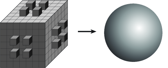
Figure 1. Embedding of the snowball.

Start with the unit cube. Divide each face into $N\times N$ squares of side-length $1/N$ (called $1/N$-squares). Put cubes of side-length $1/N$ on some $1/N$-squares. We require that the small cubes are added in a pattern that respects the symmetry group of the cube. This means that on every side of the unit cube the pattern is the same, as well as that on each side we can rotate and reflect without changing the pattern. Figure 1 illustrates one example with $N=7$. The boundary of the resulting domain is a polyhedral surface built from $1/N$-squares, called the first approximation of the snowsphere. Subdivide each $1/N$-square again, and put cubes of side-length $1/N^{2}$ on them in the same pattern as before. Thus we obtain a domain bounded by a polyhedral surface built from $1/N^{2}$-squares (the second approximation of the snowsphere). Iterating this process we get a snowball $\mathcal{B}$ as (the closure of) the limiting domain, with a snowsphere $\mathcal{S}$ as its boundary.

Remarks.

One has to impose relatively mild conditions to ensure that the snowsphere $\mathcal{S}$ is a topological sphere, i.e., does not have self-intersections. In every step a different pattern and a different number $N_{j}$ may be used. We then have to assume that $\sup_{j}N_{j}<\infty$.

The main theorem we prove is the following.

Theorem 1.

For every snowball $\mathcal{B}$ there is a quasiconformal map

$$f\colon\mathbb{R}^{3}\to\mathbb{R}^{3}$$

that maps $\mathcal{B}$ to the unit ball $\mathbb{B}$.

Obviously then $f(\mathcal{S})=\mathbb{S}$. The proof is broken up into two parts.

Theorem 1A.

Every snowsphere $\mathcal{S}$ can be mapped to the unit sphere $\mathbb{S}$ by a quasisymmetry

$$f\colon\mathcal{S}\to\mathbb{S}.$$

This theorem will be proved in Section 3. We first equip the $j$-th approximation of the snowsphere with a conformal structure in a standard way. By the uniformization theorem it is conformally equivalent to the sphere. The proof of the quasisymmetry of the map $f$ relies essentially on two facts. The first is that the number of small squares intersecting in a vertex is bounded by $6$ throughout the whole construction. This means that if one looks at a square and adjacent squares, only finitely many combinatorially different situations occur. The second ingredient is that combinatorial equivalence implies conformal equivalence. Thus in combinatorially equivalent sets the distortion is comparable by Koebe’s theorem. Only finitely many constants appear, one for each of the (finitely many) combinatorial situations of suitable neighborhoods. This idea already appeared in [Mey02].

The remainder of the paper concerns the extension of the map $f$ to $f\colon\mathbb{R}^{3}\to\mathbb{R}^{3}$. The construction is explicit, though somewhat technical. In Section 4 some maps and extensions that will be useful later on are provided. The snowball is decomposed in Section 5 in a Whitney-type fashion, where the size of a piece is comparable to its distance from the boundary (the snowsphere). In Section 6 the pieces are mapped to the unit ball and reassembled there. One has to make sure that $f$ agrees on intersecting pieces (is well defined). The explicit construction of the map $f\colon\mathcal{S}\to\mathbb{S}$ allows us to control distortion.

In Section 7 the remaining part of Theorem 1 is proved.

Theorem 1B.

The map $f$ from Theorem 1A can be extended to a quasiconformal map

$$f\colon\mathbb{R}^{3}\to\mathbb{R}^{3}.$$

Thus one obtains a large class of quasispheres. The Xmas tree example from [Mey02] shows that there are quasispheres (in $\mathbb{R}^{3}$) having Hausdorff dimension arbitrarily close to $3$. On the other hand, one can construct quasispheres having Hausdorff dimension $2$ that are not Ahlfors $2$-regular.

1.4. Notation

$\widehat{\mathbb{C}}=\mathbb{C}\cup\{\infty\}$ is the Riemann sphere, $\mathbb{S}=\{x\in\mathbb{R}^{3}:\lvert x\rvert=1\}$ the unit sphere, $\mathbb{B}=\{x\in\mathbb{R}^{3}:\lvert x\rvert\leq 1\}$ the (closed) unit ball, $\mathbb{D}=\{z\in\mathbb{C}:\lvert z\rvert<1\}$ the unit disk.

The Euclidean norm in $\mathbb{R}^{n}$ is denoted by $\lvert x\rvert$, the Euclidean metric by $\lvert x-y\rvert$. The sphere $\mathbb{S}$ and the unit ball $\mathbb{B}$ are equipped with the Euclidean metric inherited from $\mathbb{R}^{3}$, unless otherwise noted. We identify $\widehat{\mathbb{C}}$ with $\mathbb{S}$, meaning $\widehat{\mathbb{C}}$ is equipped with the chordal metric. Maximum norm and metric are denoted by $\lVert x\rVert_{\infty}$ and $\lVert x-y\rVert_{\infty}$.

For two non-negative expressions $f,g$ we write $f\asymp g$ if there is a constant $C\geq 1$ such that $\frac{1}{C}g\leq f\leq Cg$. We will often refer to $C$ by $C(\asymp)$, for example we will write $C(\asymp)=C(n,m)$ if $C$ depends on $n$ and $m$.

Similarly we write $f\lesssim g$ or $g\gtrsim f$ for two non-negative expressions $f,g$ if there is a constant $C>0$ such that $f\leq Cg$. The constant $C$ is referred to as $C(\lesssim)$ or $C(\gtrsim)$.

The interior of a set $S$ is denoted by $\operatorname{int}S$, the closure by $\operatorname{clos}S$, while $U_{\epsilon}(S):=\{x:\operatorname{dist}(x,S)<\epsilon\}$ denotes the open $\epsilon$-neighborhood of a set $S$.

Let

(1.2) $$d_{A}(B) :=\inf\{\epsilon:B\subset U_{\epsilon}(A)\}$$

$$=\sup\{\operatorname{dist}(b,A):b\in B\}.$$

The Hausdorff distance between two sets $A,B$ is

$$\operatorname{Hdist}(A,B):=\max\{d_{A}(B),d_{B}(A)\}.$$

Lemma 1.1.

Let $A,B,C$ be arbitrary sets; then

(1.3) $$\operatorname{Hdist}(A,B) \leq\operatorname{Hdist}(A,C)+\operatorname{Hdist}(C,B),$$

(1.4) $$\operatorname{dist}(A,B) \geq\operatorname{dist}(A,C)-d_{C}(B)$$

(1.5) $$\geq\operatorname{dist}(A,C)-\operatorname{Hdist}(C,B).$$

Proof.

The first inequality is clear.

To see the second inequality, let $b\in B$ be arbitrary; then

$$\operatorname{dist}(A,C) =\inf_{\begin{subarray}{c}a\in A\\ c\in C\end{subarray}}\lvert a-c\rvert\leq\inf_{a\in A}\lvert a-b\rvert+\inf_{c\in C}\lvert b-c\rvert$$

$$=\inf_{a\in A}\lvert a-b\rvert+\operatorname{dist}(b,C)\leq\inf_{a\in A}\lvert a-b\rvert+d_{C}(B).$$

Taking the infimum with respect to $b\in B$ yields (1.4). The last inequality follows from $d_{A}(B)\leq\operatorname{Hdist}(A,B)$. ∎

We identify $\mathbb{R}^{2}$ with the $xy$-plane in $\mathbb{R}^{3}$; similarly when writing “$[0,1]^{2}\subset\mathbb{R}^{3}$”, we identify $[0,1]^{2}$ with $[0,1]^{2}\times\{0\}$, etc.

1.5. Polyhedral Surfaces

Snowspheres will be approximated by polyhedral surfaces. We recall some well-known facts. Let $S\subset\mathbb{R}^{3}$ be a polyhedral surface homeomorphic to the sphere $\mathbb{S}$. The following is Theorem 17.12 in [Moi77].

Theorem (PL-Schönflies Theorem for $\mathbb{R}^{3}$).

There is a PL-(piecewise linear) homeomorphism $h\colon\mathbb{R}^{3}\to\mathbb{R}^{3}$ such that $h(\partial[0,1]^{3})=S$.

Corollary 1.2.

Let $S$ be a polyhedral surface homeomorphic to $\mathbb{S}$. Then the closure of the bounded component of $\mathbb{R}^{3}\setminus S$ is bi-Lipschitz equivalent to the cube $[0,1]^{3}$.

2. Snowballs and Snowspheres

2.1. Generators

We first introduce some terminology. By the pyramid above (denoted by $\mathcal{P}^{+}$) the unit square $[0,1]^{2}\subset\mathbb{R}^{2}\subset\mathbb{R}^{3}$ we mean the pyramid with base $[0,1]^{2}$ and tip $(\frac{1}{2},\frac{1}{2},\frac{1}{2})$ (which is the center of the unit cube $[0,1]^{3}$). The pyramid below the unit square is the one with base $[0,1]^{2}$ and tip $(\frac{1}{2},\frac{1}{2},-\frac{1}{2})$. We denote by $\mathcal{P}$ the double pyramid of the unit square, which is the union of the two pyramids defined above. The double pyramid $\mathcal{P}(Q)$ of any square $Q\subset\mathbb{R}^{3}$ is defined as the image of the double pyramid $\mathcal{P}$ under a similarity (of $\mathbb{R}^{3}$) that maps the unit square to $Q$. If we give $Q$ an orientation we also speak of its pyramids above and below.

Consider two distinct unit squares in the grid $\mathbb{Z}^{3}$. Their double pyramids intersect at most in a (common) face, which means they have disjoint interiors.

An $N$-generator (for an integer $N\geq 2$) is a polyhedral surface $G\subset\mathbb{R}^{3}$ built from squares of side-length $\frac{1}{N}=\delta$ ($\delta$-squares). We require:

1. $G$ is homeomorphic to the unit square $[0,1]^{2}$.

2. The boundary of $G$ (as a surface) consists of the four sides of the unit square:

   $$\partial G=\partial[0,1]^{2}.$$

3. $G$ is contained in the double pyramid $\mathcal{P}$ and intersects its boundary only in the boundary (the four edges) of the unit square:

   $$G\subset\mathcal{P}\mbox{ and }G\cap\partial\mathcal{P}=\partial[0,1]^{2}.$$

4. The angle between two adjacent $\delta$-squares is a multiple of $\frac{\pi}{2}$ (so it is $\frac{\pi}{2},\pi$, or $\frac{3\pi}{2}$).

5. The generator $G$ is symmetric, meaning it is invariant under orientation preserving symmetries of the unit square $[0,1]^{2}$; more precisely under rotations by multiples of $\pi/2$ around the axis $\{(\frac{1}{2},\frac{1}{2},z)\}$, and reflections on the planes $\{x=\frac{1}{2}\},\{y=\frac{1}{2}\},\{x=y\}$, and $\{y=1-x\}$.

Definition 2.1.

We say a surface that can be decomposed into squares having edges in a grid $\delta\mathbb{Z}^{3}$ lives in the grid $\delta\mathbb{Z}^{3}$. Similarly, we say a domain lives in a grid $\delta\mathbb{Z}^{3}$ if this is true for its boundary.

So an $N$-generator lives in the grid $\frac{1}{N}\mathbb{Z}^{3}$. For a given $N$ there can be only finitely many such generators.

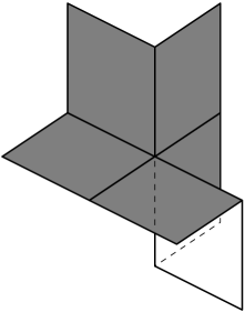
Figure 2. The forbidden configuration.

One last assumption about generators will be made, though it is not strictly necessary. However, it will simplify the decomposition of the snowball $\mathcal{B}$ in Section 5 considerably. We do not allow the situation indicated in Figure 2 to occur. To be more precise consider an interior vertex of $G$, meaning a point $v\in(G\cap\delta\mathbb{Z}^{3})\setminus\partial[0,1]^{2}$. At $v$ it is possible that $3,4,5$ or $6$ $\delta$-squares intersect. We do not allow $6$ $\delta$-squares around $v$ which form successive angles of $\pi,\frac{3}{2}\pi,\pi/2,\pi,\frac{3}{2}\pi,\pi/2$. All other (allowed) possibilities (up to rotations/reflections) of how $\delta$-squares may intersect in a vertex are indicated in Figure 10.

1. The generator $G$ does not contain a forbidden configuration as in Figure 2.

In the next section we will define the approximations $\mathcal{S}_{j}$ of the snowsphere, which will be built successively from generators.

Remarks.

• Condition (i) in the definition of a generator is clearly necessary for $\mathcal{S}_{j}$ to be homeomorphic to the sphere $\mathbb{S}$.

• Condition (ii) enables us to replace the $\delta_{j}$-squares by a scaled copy of a generator.

• The third condition (iii) guarantees that the approximations $\mathcal{S}_{j}$ (and ultimately the snowsphere $\mathcal{S}$) are topological spheres. See the next subsection.

• The fourth condition (iv) is equivalent to saying that a generator lives in the grid $\frac{1}{N}\mathbb{Z}^{3}$. It is most likely superfluous. However, we were not able to find a convincing argument for this.

• The fifth condition (v) is necessary for our method to work. Avoiding it would be very desirable. Indeed, tackling the non-symmetric case might be the first step towards a general theory.

• The last condition is imposed to avoid more technicalities when decomposing the snowball in Section 5.2. See the Remark on page Remark.

2.2. Approximations of the Snowsphere

A snowball $\mathcal{B}$ is a three-dimensional analog of the domain bounded by the snowflake curve. It is a compact set in $\mathbb{R}^{3}$ homeomorphic to the closed unit ball $\mathbb{B}=\{x\in\mathbb{R}^{3}:\lvert x\rvert\leq 1\}$. The corresponding snowsphere $\mathcal{S}:=\partial\mathcal{B}$ is homeomorphic to the unit sphere $\mathbb{S}=\{x\in\mathbb{R}^{3}:\lvert x\rvert=1\}=\partial\mathbb{B}$. We will obtain $\mathcal{S}$ as the Hausdorff limit of approximations $\mathcal{S}_{j}$. To obtain $\mathcal{S}_{j+1}$ from $\mathcal{S}_{j}$ we replace small squares by scaled generators.

The $0$-th approximation of the snowsphere $\mathcal{S}_{0}$ is the surface of the unit cube, $\mathcal{S}_{0}:=\partial[0,1]^{3}$. Now replace each of the six faces of $\mathcal{S}_{0}$ by a rotated copy of an $N_{1}$-generator to get $\mathcal{S}_{1}$, the first approximation of the snowsphere. It is a polyhedral surface built from $\frac{1}{N_{1}}$-squares. We construct $\mathcal{S}_{2}$ by replacing each $\frac{1}{N_{1}}$-square of $\mathcal{S}_{1}$ by a scaled (by the factor $\frac{1}{N_{1}}$) and rotated copy of an $N_{2}$-generator. Inductively the $j$-th approximations of the snowsphere $\mathcal{S}_{j}$ are constructed. Each $\mathcal{S}_{j}$ is a polyhedral surface built from squares of side-length

(2.1) $$\delta_{j}:=\frac{1}{N_{1}}\times\dots\times\frac{1}{N_{j}}.$$

It will be convenient to set $\delta_{0}:=1$ and $\delta_{\infty}:=0$. Note that when constructing $\mathcal{S}_{j+1}$ from $\mathcal{S}_{j}$ each $\delta_{j}$-square is replaced by the same $N_{j+1}$-generator. We do however allow two $\delta_{j}$-squares $Q_{1}$ and $Q_{2}$ to be replaced by scaled copies of the $N_{j+1}$-generator with different orientation. So the generator can “stick out” on one square and “point inwards” on another. In each step a different generator may be used. We do require that

(2.2) $$N_{\max}:=\max_{j}{}N_{j}<\infty.$$

This implies that only finitely many different generators are used. The construction may be paraphrased as follows. Pick a finite set of generators. In each step pick a generator from this set to construct the next approximation.

All relevant constants will depend on $N_{\max}$ only. Such a constant is called uniform.

Lemma 2.2.

The approximations $\mathcal{S}_{j}$ are topological spheres.

Proof.

Let $g_{0}\colon\mathbb{S}\to\mathcal{S}_{0}=\partial[0,1]^{3}$ be a homeomorphism. For every $N_{j+1}$-generator $G_{j+1}$ we can find a homeomorphism $[0,1]^{2}\to G_{j+1}$ which is constant on $\partial[0,1]^{2}$. Apply this homeomorphism to every $\delta_{j}$-square in $\mathcal{S}_{j}$ to get a continuous and surjective map

$$g_{j+1}\colon\mathcal{S}_{j}\to\mathcal{S}_{j+1},$$

which is constant on the $1$-skeleton of $\mathcal{S}_{j}$ (edges of $\delta_{j}$-squares in $\mathcal{S}_{j}$). To see injectivity consider two distinct $\delta_{j}$-squares $Q,Q^{\prime}\subset\mathcal{S}_{j}$. Then $G:=g_{j+1}(Q),G^{\prime}:=g_{j+1}(Q^{\prime})\subset\mathcal{S}_{j+1}$ are scaled (by $\delta_{j}$) copies of the $N_{j+1}$-generator. Note that they are contained in the double pyramids, $G\subset\mathcal{P}(Q),G^{\prime}\subset\mathcal{P}(Q^{\prime})$. By condition (iii) of generators

$$g_{j+1}(\operatorname{int}Q) =\operatorname{int}G\subset\operatorname{int}\mathcal{P}(Q)\text{ and}$$

$$g_{j+1}(\operatorname{int}Q^{\prime}) \subset\operatorname{int}\mathcal{P}(Q^{\prime}).$$

Thus $g_{j+1}(\operatorname{int}Q)\cap g_{j+1}(\operatorname{int}Q^{\prime})=\operatorname{int}\mathcal{P}(Q)\cap\operatorname{int}\mathcal{P}(Q^{\prime})=\emptyset$. Note also that $\operatorname{int}\mathcal{P}(Q)$ does not intersect the $1$-skeleton of $\mathcal{S}_{j}$. Thus $g_{j+1}$ is injective, hence a homeomorphism. This shows by induction that every approximation $\mathcal{S}_{j}$ is a topological sphere. ∎

The approximations $\mathcal{S}_{j}$ are polyhedral surfaces. Thus $\mathbb{R}^{3}\setminus\mathcal{S}_{j}$ has two components by the PL-Schönflies theorem.

Call the edges/vertices of a $\delta_{j}$-square in $\mathcal{S}_{j}$ $\delta_{j}$-edges/vertices. Then the approximations $\mathcal{S}_{j}$ form a cell complex in a natural way. Namely the $\delta_{j}$-squares/edges/vertices in $\mathcal{S}_{j}$, are the $2$-, $1$-, and $0$-cells.

2.3. Snowspheres

Note that $\operatorname{Hdist}(\mathcal{S}_{j},\mathcal{S}_{j+1})\leq\delta_{j}\leq 2^{-j}$. Thus we can define the snowsphere $\mathcal{S}$ as the limit of the approximations $\mathcal{S}_{j}$ in the Hausdorff topology. It is possible to prove that $\mathcal{S}$ is a topological sphere as in Lemma 2.2. However we would have to make additional assumptions on the maps $g_{j}$. Therefore we postpone the proof that $\mathcal{S}$ is homeomorphic to $\mathbb{S}$ until Corollary 3.11.

We call the closure of the bounded components of $\mathbb{R}^{3}\setminus\mathcal{S}$ the snowball $\mathcal{B}$. It will follow from Theorem 1B that $\mathcal{B}$ is homeomorphic to a closed ball. See also Corollary 5.4.

When a snowsphere $\mathcal{S}$ is given, “$N_{j}$-generator” will always refer to the one used in the $j$-th step of the construction.

It will often be convenient to consider only one “face” $\mathcal{T}$ of the snowsphere, i.e., the part of it that was constructed from one of the sides of the surface of the unit cube. More precisely let $\mathcal{T}_{0}=[0,1]^{2}$ be the unit square, $\mathcal{T}_{1}$ be the $N_{1}$-generator, $\mathcal{T}_{2}$ the surface obtained by replacing each $\frac{1}{N_{1}}$-square by a scaled copy of the $N_{2}$-generator, and so on. Then $\mathcal{T}:=\lim_{j}\mathcal{T}_{j}$ in the Hausdorff topology.

 

(a) Generator with enclosing pyramid.

(b) Pyramids on each $\frac{1}{N_{1}}$-square.

Figure 3. Generator and pyramids in the grid $\frac{1}{N_{1}}\mathbb{Z}^{3}$.

Consider the $N_{1}$-generator ($=\mathcal{T}_{1}$) and its enclosing double pyramid $\mathcal{P}$. Figure 3(a) shows a 2-dimensional picture where we cut through the middle (along the plane $y=\frac{1}{2}$). Only the upper pyramid is depicted. For convenience the picture also indicates the grid $\frac{1}{N_{1}}\mathbb{Z}^{3}$ (or rather its 2-dimensional intersection $\frac{1}{N_{1}}\mathbb{Z}^{2}$). We note that

• the height of $\mathcal{T}_{1}$ is at most $\frac{1}{2}-\frac{3}{2}\frac{1}{N_{1}}$.

Here the precise meaning of “height” is the maximal distance of a point in the generator from the base square $[0,1]^{2}$. This is easily seen from Figure 3(a). Indeed, the next layer of $\frac{1}{N_{1}}$-cubes (having height $\frac{1}{2}-\frac{1}{2N_{1}}$) would intersect the boundary of the double pyramid (or lie outside). If $N_{1}$ is even the height is at most $\frac{1}{2}-\frac{2}{N_{1}}$.

The projection of any generator to the $xy$-plane is the square $[0,1]^{2}$. Thus we note the following consequence of the above:

(2.3) $$\operatorname{Hdist}_{\infty}(\mathcal{S}_{j},\mathcal{S}_{j+1})\leq\operatorname{Hdist}(\mathcal{S}_{j},\mathcal{S}_{j+1})\leq\left(\frac{1}{2}-\frac{3}{2}\frac{1}{N_{j+1}}\right)\delta_{j}.$$

Here “$\operatorname{Hdist}_{\infty}$” is the Hausdorff distance taken with respect to the maximum metric; see Subsection 5.2.

Put pyramids on the $\frac{1}{N_{1}}$-squares of $\mathcal{T}_{1}$. These stay inside the double pyramid $\mathcal{P}$; see Figure 3(b). Consider the pyramids of interior $\frac{1}{N_{1}}$-squares, i.e., squares that do not intersect the boundary of the unit square $\partial[0,1]^{2}$. These have distance at least $\frac{\sqrt{2}}{2}\frac{1}{N_{1}}$ from the surface of the enclosing double pyramid $\mathcal{P}$.

If we now replace each $\frac{1}{N_{1}}$-square by the $N_{2}$-generator to get $\mathcal{T}_{2}$, we see that $\mathcal{T}_{2}$ stays inside the $\frac{1}{N_{1}}$-pyramids depicted in Figure 3(b). Induction yields that all $\mathcal{T}_{j}$ and hence $\mathcal{T}$ are contained in the double pyramid $\mathcal{P}$. Furthermore, if $Q_{j}$ is an interior $\delta_{j}$-square of $\mathcal{T}_{j}$, then the double pyramid of $Q_{j}$ has distance $\sqrt{2}\delta_{j}/2$ from the boundary $\partial\mathcal{P}$. We conclude

• $\mathcal{T}$ is contained in the double pyramid $\mathcal{P}$ and intersects its boundary only in the boundary of the unit square:

  $$\mathcal{T}\subset\mathcal{P}\mbox{ and }\mathcal{T}\cap\partial\mathcal{P}=\partial[0,1]^{2}.$$

• The height of $\mathcal{T}$ is at most $\frac{1}{2}-\frac{1}{N_{1}}\leq\frac{1}{2}-\frac{1}{N_{\max}}$. ($*$)

Again by “height” we mean the maximal distance of a point in $\mathcal{T}$ from the base square $[0,1]^{2}$. The projection of $\mathcal{T}$ to the $xy$-plane is still the square $[0,1]^{2}$. Thus we conclude by ($*$) above that the Hausdorff distance between $\mathcal{S}_{j}$ and $\mathcal{S}$ satisfies

(2.4) $$\operatorname{Hdist}(\mathcal{S}_{j},\mathcal{S})\leq\delta_{j}\left(\frac{1}{2}-\frac{1}{N_{\max}}\right).$$

Recall that the $j$-th approximation of the snowsphere $\mathcal{S}_{j}$ was built from $\delta_{j}$-squares. The part of the snowsphere which was constructed by replacing one such $\delta_{j}$-square $Q\subset\mathcal{S}_{j}$ (infinitely often) by generators is called a cylinder of order $j$ (or $j$-cylinder). By the previous argument this cylinder is contained in the double pyramid $\mathcal{P}(Q)$ of $Q$, so we can define more precisely

$$X_{j}=X_{j}(Q):=\mathcal{P}(Q)\cap\mathcal{S}$$

to be the $j$-cylinder with base $Q$. The set of all $j$-cylinders is denoted by $\mathbf{X}_{j}$. It will be convenient to let $\mathcal{S}$ be the (only) $-1$-cylinder. Set $\delta_{-1}:=2$ so that

$$\operatorname{diam}X_{j}\leq\sqrt{2}\delta_{j},$$

for every $j$-cylinder $X_{j}$.

For every point $x\in\mathcal{S}$ there is a (not necessarily unique) sequence $(X_{j})_{j\in\mathbb{N}}$, where $X_{j}$ is a $j$-cylinder such that

(2.5) $$X_{0}\supset X_{1}\supset X_{2}\supset\dots\supset\bigcap_{j}X_{j}=\{x\}.$$

If we use the same generator with the same orientation throughout the construction of $\mathcal{S}$, we get a self-similar snowsphere. In that case each cylinder is a (scaled and rotated) copy of $\mathcal{T}$.

Now consider a $\delta_{j}$-square $Q\subset\mathcal{S}_{j}$, its double pyramid $\mathcal{P}(Q)$, and its cylinder $X_{j}=X_{j}(Q)$. Then $X_{j}$ is contained in $\mathcal{P}(Q)$ and intersects it only in the boundary of $Q$ by the same reasoning as above:

$$X_{j}\cap\mathcal{P}(Q)=\partial Q.$$

Now let $R\subset\mathcal{S}_{j}$ be a second $\delta_{j}$-square. Their double pyramids $\mathcal{P}(Q)$ and $\mathcal{P}(R)$ intersect only at the boundary: $\mathcal{P}(Q)\cap\mathcal{P}(R)=\partial\mathcal{P}(Q)\cap\partial\mathcal{P}(R)$ (they have disjoint interior). It follows that the cylinders $X_{j}(Q)\subset\mathcal{P}(Q)$ and $X_{j}(R)\subset\mathcal{P}(R)$ intersect only in the intersection of $Q$ and $R$:

$$X_{j}(Q)\cap X_{j}(R)=Q\cap R.$$

Thus two distinct non-disjoint $j$-cylinders can intersect in an edge or a vertex (contained in $\delta_{j}\mathbb{Z}^{3}$). Hence the $j$-cylinders form a cell complex in a natural way.

Lemma 2.3.

The set of $\delta_{j}$-squares in the approximations $\mathcal{S}_{j}$ is combinatorially equivalent to the set of $j$-cylinders. More precisely map each $\delta_{j}$-edge/vertex to itself and each $\delta_{j}$-square $Q\subset\mathcal{S}_{j}$ to its cylinder $X_{j}(Q)\in\mathbf{X}_{j}$,

$$Q\mapsto X_{j}(Q).$$

This map is a cell complex isomorphism.

2.4. Combinatorial Distance on $\mathcal{S}$

As a subset of $\mathbb{R}^{3}$, the snowsphere $\mathcal{S}$ inherits the Euclidean metric that we denote by $|x-y|$. Often it will be convenient to describe distances in purely combinatorial terms. Given points $x,y\in\mathcal{S}$ let

(2.6) $$j(x,y):=\min\{j:\text{ there exist disjoint }j\text{-cylinders }X_{j}\ni x,Y_{j}\ni y\}.$$

One may view $\mathcal{S}$ as the Gromov-Hausdorff limit of $j$-cylinders. The $j=j(x,y)$-th approximation $\mathcal{S}_{j}$ is the first in which it is possible to distinguish $x$ and $y$.

Lemma 2.4.

For all $x,y\in\mathcal{S}$ we have

(2.7) $$\lvert x-y\rvert\asymp\delta_{j},$$

where $j=j(x,y)$ and a constant $C(\asymp)=C(N_{\max})$.

Proof.

Let $x,y\in\mathcal{S}$ be arbitrary, and let $j:=j(x,y)$. Consider $(j-1)$-cylinders $X_{j-1}\ni x$ and $Y_{j-1}\ni y$. Then $X_{j-1}\cap Y_{j-1}\neq\emptyset$, by the definition of $j(x,y)$.

Therefore

(2.8) $$|x-y|\leq\operatorname{diam}X_{j-1}+\operatorname{diam}Y_{j-1}=\sqrt{2}\delta_{j-1}+\sqrt{2}\delta_{j-1}\leq 2\sqrt{2}N_{\max}\delta_{j}.$$

For the other inequality let $X_{j}\ni x$ and $Y_{j}\ni y$ be disjoint $j$-cylinders. Note that two disjoint $j$-cylinders are closest when their bases are opposite faces of a $\delta_{j}$-cube. Their distance then is at least

$$\delta_{j}-2\delta_{j}\left(\frac{1}{2}-\frac{1}{N_{\max}}\right)=\frac{2\delta_{j}}{N_{\max}},$$

which is the distance of base squares $-$ twice the height of $j$-cylinders, by Subsection 2.3. Hence

(2.9) $$|x-y|\geq\operatorname{dist}(X_{j},Y_{j})\geq\frac{2\delta_{j}}{N_{\max}},$$

which finishes the proof. ∎

The last lemma shows that $\delta(x,y):=\delta_{j(x,y)}$ is a quasimetric. However $\delta(x,y)$ will violate the triangle inequality.

2.5. Example

Our main example to illustrate our construction will be the self-similar snowball with generator as illustrated in Figure 4. It is the unit square divided into $25$ $\frac{1}{5}$-squares where we put a $\frac{1}{5}$-cube onto the middle square.

Figure 4. Generator used for our main example.

Notation.

When referring to this particular example we will always use “$\;\,\widehat{}\;\,\,$”, i.e., $\widehat{\mathcal{S}}$ denotes this snowsphere, $\widehat{\mathcal{S}}_{j}$ its $j$-th approximation, and so on. Then $\widehat{\delta}_{j}=5^{-j}$.

3. Uniformizing the Snowsphere

3.1. Introduction

In this section we map the snowsphere $\mathcal{S}$ to the unit sphere $\mathbb{S}$ by a quasisymmetry $f$, i.e., prove Theorem 1A. We call $f$ a uniformization of the snowsphere $\mathcal{S}$. Recall from equation (2.5) that for every point $x\in\mathcal{S}$ there is a sequence $X_{0}\supset X_{1}\supset X_{2}\supset\dots,\;X_{j}\in\mathbf{X}_{j}$, such that $\bigcap_{j}X_{j}=\{x\}$. It will therefore be enough to map the $j$-cylinders $X_{j}\subset\mathcal{S}$ to $j$-tiles $X^{\prime}_{j}\subset\mathbb{S}$, which will again satisfy $X^{\prime}_{0}\supset X^{\prime}_{1}\supset X^{\prime}_{2}\supset\dots$ . “Cylinders” live in the snowsphere $\mathcal{S}$ and “tiles” on the unit sphere $\mathbb{S}$. Generally objects in $\mathbb{S}$ will be denoted with a “prime” ($X^{\prime},x^{\prime}$, and so on), to distinguish them from objects in the snowsphere $\mathcal{S}$ and its approximations $\mathcal{S}_{j}$. We will then define

(3.1) $$f(x)=x^{\prime},\;\text{ where }\{x^{\prime}\}=\bigcap_{j}X^{\prime}_{j}.$$

The decomposition of the unit sphere $\mathbb{S}$ into $j$-tiles $X^{\prime}_{j}$ is done by using the uniformization of the $j$-th approximation of the snowsphere $\mathcal{S}_{j}$.

The proof that the map $f$ is a quasisymmetry relies on two facts. First, at most $6$ $j$-cylinders (and thus $j$-tiles) can intersect in a common vertex. Second, two sets of $j$-tiles and $k$-tiles which “have the same combinatorics” are actually conformally equivalent. The quasisymmetry is then essentially an easy consequence of the Koebe distortion theorem.

3.2. Uniformizing the approximations $\mathcal{S}_{j}$

Consider the $j$-th approximation $\mathcal{S}_{j}$ of the snowsphere $\mathcal{S}$. This is a polyhedral surface where each face is a $\delta_{j}$-square. We will view $\mathcal{S}_{j}$ as a Riemann surface. To do this we need conformal coordinates on $\mathcal{S}_{j}$, meaning that changes of coordinates are conformal maps.

3.2.1. Conformal Coordinates on the Approximations $\mathcal{S}_{j}$

• For each $\delta_{j}$-square $Q$ the affine, orientation preserving map $\operatorname{int}Q\to\operatorname{int}[0,1]^{2}$ is a chart.

• For two neighboring $\delta_{j}$-squares $P$, $Q$ (i.e., ones which share an edge), the map

  $$\operatorname{int}(P\cup Q)\to\operatorname{int}([0,2]\times[0,1]),$$

  which maps $P$ (affinely, orientation preserving) to $[0,1]^{2}$, $Q$ (affinely, orientation preserving) to $[1,2]\times[0,1]$, and $P\cap Q$ to $\{1\}\times[0,1]$, is a chart. Using (hopefully) intuitive notation we sometimes write: $P\cup Q$ may be mapped conformally to $\square\!\square$. So $P$ and $Q$ are conformal reflections of each other in these coordinates.

• Consider a vertex $v$. Let $Q_{1},\dots,Q_{n}$ be the $\delta_{j}$-squares containing $v$, labeled with positive orientation around $v$. Map the neighborhood $\operatorname{int}(\bigcup Q_{k})$ of $v$ by $z\mapsto z^{4/n}$. More precisely the chart is constructed as follows. Map $Q_{1}$ to the unit square $[0,1]^{2}$ as above with $v\mapsto 0$. The unit square $[0,1]^{2}$ is subsequently mapped by the map $z\mapsto z^{4/n}$. Map the second $\delta_{j}$-square $Q_{2}$ as before to $[0,1]^{2}$ (again with $v\mapsto 0$), which is then mapped by $z\mapsto e^{2\pi i/n}z^{4/n}$. Alternatively we could have mapped $Q_{2}$ to $[-1,0]\times[0,1]$ and subsequently by the map $z\mapsto z^{4/n}$. So the image of $Q_{2}$ is a conformal reflection of the image of $Q_{1}$, along the shared side $[0,e^{2\pi i/n}]$. The third $\delta_{j}$-square $Q_{3}$ is mapped to $[0,1]^{2}$, and then by $z\mapsto e^{4\pi i/n}z^{4/n}$ and so on. Again the image of $Q_{3}$ is a reflection of the image of $Q_{2}$, analogously for the other $\delta_{j}$-squares. Since each mapped $\delta_{j}$-square forms an angle of $2\pi/n$ at $0$, the last matches up with the first, meaning they are conformal reflections of each other.

It is immediate that changes of coordinates are conformal. The charts are illustrated in Figure 5.

\psfrag{a}[2]{$z\mapsto z^{4/3}$}\includegraphics{3quadratsecond.eps}

\psfrag{a}[2]{$z\mapsto z^{4/3}$}\psfrag{b}[2]{$z\mapsto z^{4/5}$}\includegraphics{5quadratsecond.eps}

Figure 5. Conformal coordinates on a polyhedral surface.

With these charts each approximation $\mathcal{S}_{j}$ of the snowsphere is a compact, simply connected Riemann surface. Therefore $\mathcal{S}_{j}$ is conformally equivalent to the sphere $\widehat{\mathbb{C}}$ by the uniformization theorem. Identify $\widehat{\mathbb{C}}$ with $\mathbb{S}\subset\mathbb{R}^{3}$. It is not yet clear, however, what the relation is between uniformizations of different approximations $\mathcal{S}_{j}$ and $\mathcal{S}_{k}$. We therefore construct the uniformizations of the $\mathcal{S}_{j}$ inductively, where this will be apparent.

Start with $\mathcal{S}_{0}$, which is the surface of the unit cube $\partial[0,1]^{3}$. Equip $\mathcal{S}_{0}$ with a conformal structure as above and map it conformally to the Riemann sphere $\widehat{\mathbb{C}}$ using the uniformization theorem. The images of the faces of $\mathcal{S}_{0}$ decompose the sphere $\widehat{\mathbb{C}}$ into $0$-tiles. Edges and vertices of those $0$-tiles are the images of edges and vertices of the faces of $\mathcal{S}_{0}$. By symmetry we can assume that the vertices of the $0$-tiles form a cube, i.e., all $0$-tiles have the same size.

Denote the set of all such $0$-tiles by $\mathbf{X}^{\prime}_{0}$. Each tile $X^{\prime}\in\mathbf{X}^{\prime}_{0}$ is conformally a square, meaning we can map it conformally to the unit square $[0,1]^{2}$, where vertices map to vertices. Consider two neighboring tiles $X^{\prime},Y^{\prime}\in\mathbf{X}^{\prime}_{0}$ (i.e., which share an edge). By the definition of our charts they are conformal reflections of each other. So we could start with one tile and get all other tiles by repeated reflection along the edges. Such a tiling is called a conformal tiling.

Definition 3.1.

A conformal tiling of a domain $D\subset\widehat{\mathbb{C}}$ is a decomposition into tiles $D=\bigcup T$, such that:

• Each tile $T$ is a closed Jordan region, bounded by finitely many analytic arcs. Every such arc is part of the boundary of exactly two tiles.

• Two distinct tiles $T$ and $\widetilde{T}$ have disjoint interior, $\operatorname{int}T\cap\operatorname{int}\widetilde{T}=\emptyset$.

• Call the endpoints of the analytic arcs (from the boundaries of the tiles) vertices. The tiling forms a cell complex, where the tiles/analytics arcs/vertices are the $2$-,$1$-, and $0$-cells. This means in particular that distinct tiles can only intersect in the union of several such analytic arcs and vertices.

• Two tiles sharing an analytic boundary arc (neighbors) are conformal reflections along this arc.

Conformal tilings are of course preserved under conformal maps.

Now consider the $N_{1}$-generator $G_{1}$ as a Riemann surface using charts as above. Note that $\operatorname{int}G_{1}$ is simply connected, and has more than two boundary points. Thus $\operatorname{int}G_{1}$ is conformally equivalent to the unit disk $\mathbb{D}$ by the uniformization theorem. Because of symmetry, we can map $G_{1}$ conformally to the unit square $[0,1]^{2}$ (mapping vertices to vertices as usual). Figure 6 shows the uniformization of the generator $\widehat{G}$ (see Figure 4) of the example $\widehat{\mathcal{S}}$. The picture was obtained by dividing the generator along the diagonals into $4$ pieces. One such piece (a $7$-gon) was mapped to a quarter of the unit square by a Schwarz-Christoffel map, using Toby Driscoll’s Schwarz-Christoffel Toolbox (http://www.math.udel.edu/~driscoll/ software/); see [DT02]. Thus this picture (as well as following ones) is conformally correct, up to numerical errors.

The images of the $\delta_{1}$-squares in $G_{1}$ again form a tiling of the unit square $[0,1]^{2}$. Map a second copy of the uniformized generator to the square $[1,2]\times[0,1]$ (map the two tiled squares to $\square\!\square$). The tilings are symmetric with respect to the line $\{1\}\times[0,1]$ because of the symmetry of the generator $G_{1}$. So we get a conformal tiling of $\square\!\square$.

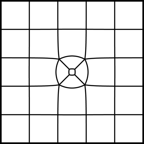
Figure 6. Uniformization of the generator $\widehat{G}$ of the snowsphere $\widehat{\mathcal{S}}$.

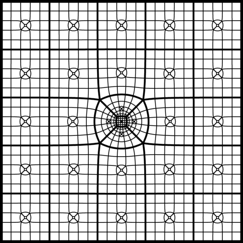
Figure 7. $2$-tiles of $\widehat{\mathcal{S}}$.

Convention.

When we have a conformal map from a square to a tile $g\colon[0,1]^{2}\to X^{\prime}$ we always assume that it maps vertices onto each other. The same normalization is used when mapping a tile to another $X^{\prime}\to Y^{\prime}$.

The uniformized generator $G_{1}$ and each $0$-tile $X^{\prime}_{0}$ are conformally equivalent to a square. So we can map the uniformization of $G_{1}$ (the unit square tiled by images of $\delta_{1}$-squares) to $X^{\prime}_{0}$. The images of the tiles of $[0,1]^{2}$ under this map are called the $1$-tiles $X^{\prime}_{1}\subset\widehat{\mathbb{C}}$. We denote the set of all $1$-tiles by $\mathbf{X}^{\prime}_{1}$.

3.2.2. Properties of the Tiling

• Every $1$-tile is conformally a square, meaning we can map it to the unit square $[0,1]^{2}$ by a conformal map (mapping vertices to vertices).

• Each $1$-tile is contained in exactly one $0$-tile.

• Two neighboring $1$-tiles $X^{\prime}_{1},Y^{\prime}_{1}$ (tiles which share an edge) may be mapped conformally to the rectangle $\square\!\square$. This is clear when $X^{\prime}_{1}$ and $Y^{\prime}_{2}$ are contained in the same $0$-tile $X^{\prime}_{0}$.

  Assume they are contained in different $0$-tiles, $X^{\prime}_{1}\subset X^{\prime}_{0}\in\mathbf{X}^{\prime}_{0}$ and $Y^{\prime}_{1}\subset Y^{\prime}_{0}\in\mathbf{X}^{\prime}_{0}$. Then $X^{\prime}_{0}\cup Y^{\prime}_{0}$ can be mapped conformally to the rectangle $\square\!\square$. In this chart the tiles in the left and right square are symmetric with respect to the line $\{1\}\times[0,1]$. So $X^{\prime}_{1}$ and $Y^{\prime}_{1}$ are conformal reflections of each other.

• The set $\mathbf{X}^{\prime}_{1}$ forms a conformal tiling of the sphere $\widehat{\mathbb{C}}$.

• Each $\delta_{1}$-square $Q\in\mathcal{S}_{1}$ is mapped to a $1$-tile. Squares which share a (vertex, edge) are mapped to $1$-tiles which share a (vertex, edge) under this map.

• The tiling $\mathbf{X}^{\prime}_{1}$ is a uniformization of the approximation $\mathcal{S}_{1}$ of the snowsphere. By this we mean the following. Map a $\delta_{1}$-square $Q$ to its corresponding $1$-tile $X^{\prime}$ by the Riemann map (normalized by mapping corresponding vertices onto each other). By reflection this extends to a neighboring $\delta_{1}$-square $\widetilde{Q}$, where it is the Riemann map to the neighboring $1$-tile $\widetilde{X}^{\prime}$ (again with the “right” normalization at vertices). The map extends to all of $\mathcal{S}_{1}$ by reflection and is well defined. The extension is conformal (with respect to the conformal structure on $\mathcal{S}_{1}$ as described above).

The above procedure is now iterated. Let the $j$-th tiling of the sphere $\widehat{\mathbb{C}}$ be given, and let the set of $j$-tiles be denoted by $\mathbf{X}^{\prime}_{j}$. We map the uniformized $N_{j+1}$-generator to each $j$-tile $X^{\prime}_{j}\in\mathbf{X}^{\prime}_{j}$ to get the $(j+1)$-tiles $X^{\prime}_{j+1}\in\mathbf{X}^{\prime}_{j+1}$. Tiles are always compact. All the above statements hold (where $0$ is replaced by $j$ and $1$ by $j+1$). Figure 7 shows the $2$-tiles for the example $\widehat{\mathcal{S}}$. It will be convenient to call the whole sphere $\mathbb{S}$ the (only) $-1$-tile. Let us record the properties of the tilings.

Lemma 3.2.

The tiles satisfy the following:

1. Each $j$-tile is conformally a square, meaning we can map it conformally to the square (mapping vertices to vertices).

2. The set of $j$-tiles forms a conformal tiling for every $j\geq 0$.

3. The $j$-th tiling is a uniformization of the approximation $\mathcal{S}_{j}$. This means there are conformal maps (with respect to the structure from Subsection 3.2.1)

   $$F_{j}\colon\mathcal{S}_{j}\to\widehat{\mathbb{C}}=\mathbb{S},$$

   such that $F_{j}(Q)\in\mathbf{X}^{\prime}_{j}$ for every $\delta_{j}$-square $Q\subset\mathcal{S}_{j}$.

4. The $(j+1)$-th tiling subdivides the $j$-th tiling. This means that for each $(j+1)$-tile $X^{\prime}_{j+1}$ there exists exactly one $j$-tile $X^{\prime}_{j}\supset X^{\prime}_{j+1}$.

5. Call the images of $\delta_{j}$-edges/vertices under the map $F_{j}$ above $j$-edges/vertices. View the $j$-th tiling as a cell complex ($j$-tiles/edges/vertices are the $2$-, $1$-, and $0$-cells). Then the $j$-th tiling, the approximation $\mathcal{S}_{j}$, and the set of $j$-cylinders are combinatorially equivalent by Lemma 2.3.

6. Inclusions of tiles and cylinders are preserved. This means the following. Consider a $\delta_{j}$-square $Q_{j}\subset\mathcal{S}_{j}$ and a $\delta_{k}$-square $Q_{k}\subset\mathcal{S}_{k}$. Let $X_{j}=X_{j}(Q_{j})\in\mathbf{X}_{j}$, $X_{k}=X_{k}(Q_{k})\in\mathbf{X}_{k}$, and $X^{\prime}_{j}=F_{j}(Q_{j})\in\mathbf{X}^{\prime}_{j}$, $X^{\prime}_{k}=F_{k}(Q_{k})\in\mathbf{X}^{\prime}_{k}$ be the corresponding cylinders (in $\mathcal{S}$) and tiles (in $\mathbb{S}$). Then

   $$X_{j}\subset X_{k}\Leftrightarrow X^{\prime}_{j}\subset X^{\prime}_{k}.$$

A neighbor of a $j$-tile $X^{\prime}_{j}$ is a $j$-tile $Y^{\prime}_{j}$ which shares an edge with $X^{\prime}_{j}$.

3.3. Construction of the Map $f\colon\mathcal{S}\to\mathbb{S}$

Recall that for any $x\in\mathcal{S}$ there is a sequence

(3.2) $$X_{0}\supset X_{1}\supset X_{2}\dots,\;X_{j}\in\mathbf{X}_{j},\;\bigcap X_{j}=\{x\}.$$

Consider the tiles $X^{\prime}_{j}:=F_{j}(X_{j})$, where $F_{j}$ are the maps from Lemma 3.2 (3). They satisfy by Lemma 3.2 (6) $X^{\prime}_{0}\supset X^{\prime}_{1}\supset X^{\prime}_{2}\dots\;$.

Lemma 3.3.

The tiles shrink to a point,

$$\operatorname{diam}X^{\prime}_{j}\to 0,\;\text{ as }j\to\infty.$$

In fact $\operatorname{diam}X^{\prime}_{j}\lesssim\lambda^{j}$, for a (uniform) constant $\lambda<1$ (and a uniform constant $C(\lesssim)$).

We postpone the proof until the next subsection. By the previous lemma we can now define $f\colon\mathcal{S}\to\mathbb{S}$ by

(3.3) $$f(x)=x^{\prime},\;\text{ where }\{x^{\prime}\}=\bigcap_{j}X^{\prime}_{j}.$$

Lemma 3.4.

The map $f$ is well defined.

Proof.

Given $x\in\mathcal{S}$ let the sequence $(X_{j})_{j\in\mathbb{N}}$ be as in (3.2). Assume now that there is a second sequence $Y_{0}\supset Y_{1}\supset\dots$, $Y_{j}\in\mathbf{X}_{j}$, satisfying $\bigcap Y_{j}=\{x\}$. Then

$$(X_{0}\cap Y_{0})\supset(X_{1}\cap Y_{1})\supset\dots,$$

where each $X_{j}\cap Y_{j}$ is compact and non-empty. Let $X^{\prime}_{j}:=F_{j}(X_{j})$, $Y^{\prime}_{j}:=F_{j}(Y_{j})$, and $\{y^{\prime}\}:=\bigcap Y^{\prime}_{j}$. By Lemma 3.2 (5) and (6)

$$(X^{\prime}_{0}\cap Y^{\prime}_{0})\supset(X^{\prime}_{1}\cap Y^{\prime}_{1})\supset\dots,$$

where each $X^{\prime}_{j}\cap Y^{\prime}_{j}$ is compact and non-empty. Thus

$$\emptyset \neq\bigcap(X^{\prime}_{j}\cap Y^{\prime}_{j})\subset\bigcap Y^{\prime}_{j}=\{y^{\prime}\}\text{ and}$$

$$\emptyset \neq\bigcap(X^{\prime}_{j}\cap Y^{\prime}_{j})\subset\bigcap X^{\prime}_{j}=\{x^{\prime}\}.$$

Thus $x^{\prime}=y^{\prime}$. ∎

3.4. Combinatorial Equivalence and Finiteness

The ideas in this subsection should be considered the “guts” of the proof of Theorem 1A. Let $v$ be a vertex of a $j$-tile; the $j$-degree of $v$ is the number of $j$-tiles containing $v$:

(3.4) $$\deg_{j}(v):=\#\{X^{\prime}\in\mathbf{X}^{\prime}_{j}:v\in X^{\prime}\}.$$

Consider $j$-edges and $j$-tiles of $\mathcal{S}_{j}$ containing $v$. Note that each such $j$-edge is incident to two $j$-tiles, and each such $j$-tile is incident to two $j$-edges. So the number of $j$-tiles containing $v$ is equal to the number of $j$-edges containing $v$. In the grid $\mathbb{Z}^{3}$ there are $6$ edges that intersect at each vertex. Thus the degree of vertices is uniformly bounded, namely

(3.5) $$\deg_{j}(v)\leq 6,$$

for all vertices $v$ and numbers $j$.

Now consider a set of $j$-tiles

(3.6) $$\mathbf{X}^{\prime}=\{X^{\prime}_{1},\dots,X^{\prime}_{n}\},\;\text{ where }X^{\prime}_{1},\dots,X^{\prime}_{n}\in\mathbf{X}^{\prime}_{j}.$$

As before view $\mathbf{X}^{\prime}$ as a cell complex $\Sigma(\mathbf{X}^{\prime})$, where $j$-tiles, $j$-edges, and $j$-vertices in $\bigcup\mathbf{X}^{\prime}$ are the $2$-, $1$-, and $0$-cells of the cell complex. A second set of $k$-tiles

(3.7) $$\mathbf{Y}^{\prime}=\{Y^{\prime}_{1},\dots,Y^{\prime}_{n}\},\;\text{ where }Y^{\prime}_{1},\dots,Y^{\prime}_{n}\in\mathbf{Y}^{\prime}_{k},$$

is said to be combinatorially equivalent to $\mathbf{X}^{\prime}$, if they are equivalent when viewed as cell complexes. More precisely, there is a cell complex isomorphism

(3.8) $$\Phi\colon\Sigma(\mathbf{X}^{\prime})\to\Sigma(\mathbf{Y}^{\prime}),$$

which is orientation preserving. The equivalence class of combinatorially equivalent sets of tiles is called the combinatorial type of $\mathbf{X}^{\prime}$. Otherwise $\mathbf{X}^{\prime}$ and $\mathbf{Y}^{\prime}$ are called combinatorially different. Combinatorial equivalence implies conformal equivalence.

Lemma 3.5.

Let $\mathbf{X}^{\prime}$ and $\mathbf{Y}^{\prime}$ as above be combinatorially equivalent. Then there is a conformal map

$$g=g_{\mathbf{X}^{\prime},\mathbf{Y}^{\prime}}\colon\operatorname{int}\bigcup\mathbf{X}^{\prime}\to\operatorname{int}\bigcup\mathbf{Y}^{\prime},$$

which maps $j$-(tiles, edges, vertices) to $k$-(tiles, edges, vertices).

Proof.

Let $\Phi$ be the cell complex isomorphism in (3.8). Without loss of generality assume that $\Phi(X^{\prime}_{i})=Y^{\prime}_{i}$, for $i=1,\dots,n$. Let $g\colon\operatorname{int}X^{\prime}_{i}\to\operatorname{int}Y^{\prime}_{i}$ be the conformal map, normalized by mapping each vertex $v\in X^{\prime}_{i}$ to the vertex $\Phi(v)\in Y^{\prime}_{i}$. Neighboring tiles (in $\mathbf{X}^{\prime}$ and $\mathbf{Y}^{\prime}$) are the conformal image of $\square\!\square$. Thus if $X^{\prime}_{i},X^{\prime}_{l}$ are neighbors, $g$ extends conformally to $\operatorname{int}(X^{\prime}_{i}\cap X^{\prime}_{l})$. Interior vertices are removable singularities. ∎

The next lemma shows how one can use the tiling to define holomorphic maps of the form $z\mapsto z^{n}$. It will be applied to a covering of our conformal tilings. Recall that a conformal tiling may be viewed as a cell complex, where the $1$-cells are the (analytic) boundary arcs of the tiles.

Lemma 3.6.

Let $V=\bigcup\{X^{\prime}\in\mathbf{X}^{\prime}\}$ and $W=\bigcup\{Y^{\prime}\in\mathbf{Y}^{\prime}\}$ be two conformal tilings, where each tile is a conformal square. Let $v\in V$ and $w\in W$ be vertices, such that the degree at $v$ (number of tiles intersecting in $v$) is a multiple of the degree at $w$,

$$\deg(v)=n\deg(w),$$

for some $n\in\mathbb{N}$. Let

$$U(v) :=\bigcup\{X^{\prime}\in\mathbf{X}^{\prime}:v\in X^{\prime}\}\setminus\bigcup\{1\text{-cells of }V\text{ not containing }v\}\text{ and}$$

$$U(w) :=\bigcup\{Y^{\prime}\in\mathbf{Y}^{\prime}:w\in Y^{\prime}\}\setminus\bigcup\{1\text{-cells of }W\text{ not containing }w\}$$

be neighborhoods of $v$ and $w$. Then there is an analytic map

$$U(v)\to U(w)$$

mapping $j$-tiles to $k$-tiles, which is conformally conjugate to $z\mapsto z^{n}$.

Proof.

Label the tiles around $v$ by $X^{\prime}_{1},\dots,X^{\prime}_{nm}$, and the tiles around $w$ by $Y^{\prime}_{1},\dots,$ $Y^{\prime}_{m}$ positively around the vertices. Map the first tile $X^{\prime}_{1}$ conformally to $Y^{\prime}_{1}$, such that $v$ is mapped to $w$. By reflection this extends conformally to map $X^{\prime}_{2}$ to $Y^{\prime}_{2}$. Continuing to extend the map in this fashion $X^{\prime}_{nm}$ gets mapped to $Y^{\prime}_{m}$. Again this extends by reflection to a conformal map from $X^{\prime}_{1}$ to $Y^{\prime}_{1}$, agreeing with the previous definition of the map on $X^{\prime}_{1}$. By changing coordinates we can write the map in the form $z\mapsto z^{n}$. ∎

Proof of Lemma 3.3.

One way to prove the lemma would be to use the rational maps that can be constructed as in [Mey02]. Since it is well known that the occurring postcritically finite rational maps are sub-hyperbolic, the statement is true in the orbifold metric (see [CG93] and [Mil99]).

We give a self-contained proof here. The following may in fact be viewed as an explicit construction of the orbifold metric. It was somewhat inspired by a conversation with W. Floyd and W. Parry.

Consider first a uniformized generator as in Figure 6. The conformal maps $g$ from the unit square to a tile are contractions in the hyperbolic metric $d_{h}(x,y)$ of $\operatorname{int}[0,1]^{2}$ by the Schwarz-Pick lemma; they are strict contractions for compact subsets of $\operatorname{int}[0,1]^{2}$.

We want to consider a neighborhood $U$ of the unit square $[0,1]^{2}$ so that we can extend the maps $g\colon[0,1]^{2}\to\text{tile}$ to $U$. By Schwarz-Pick the map $g$ will then be strictly contracting on the compact set $[0,1]^{2}\subset U$ in the hyperbolic metric of $U$.

Let the number $M\in\mathbb{N}$ be the least common multiple of all occurring degrees $\deg_{j}(v)$ (recall that this was the number of $j$-tiles intersecting in a vertex $v$). It is well known that the hyperbolic plane can be tiled with hyperbolic squares with angles $2\pi/M$ if $M\geq 5$ (see [Car54], sections 398–400). Alternatively one may construct a cell complex consisting of squares where at each vertex $M$ squares intersect, put a conformal structure on the complex (as in Subsection 3.2.1), and invoke the uniformization theorem (it is not hard to show that the type will be hyperbolic). Let $Q$ be one hyperbolic square of the tiling, and $U$ be the neighborhood consisting of all hyperbolic squares with non-empty intersection with $Q$. The hyperbolic squares in $U$ form a conformal tiling. Each vertex of $Q$ belongs to $M$ tiles.

Now consider a uniformized generator, which is a conformal tiling of the unit square $[0,1]^{2}$ as in Figure 6. Map this tiling by conformal maps to each hyperbolic square in $U$. Images of the tiles of $[0,1]^{2}$ under these maps will be denoted by $T$. The tiles $T$ are again a conformal tiling of $U$.

Let $g_{T}$ be a conformal map from the hyperbolic square $Q$ to such a tile,

(3.9) $$g_{T}\colon Q\to T\subsetneq Q.$$

By the previous lemma $g_{T}$ extends to $U$ analytically, $g_{T}\colon U\to U$. Since $Q$ is compactly contained in $U$, the map $g_{T}$ is strictly contracting on $Q$ in the hyperbolic metric $d_{U}$ of $U$ (by Schwarz-Pick, see for example [Ahl73]):

$$d_{U}(g(x_{T}),g(y_{T}))\leq\lambda_{T}d_{U}(x,y),\;\text{where }\lambda_{T}<1\text{ for all }x,y\in Q.$$

Since there are only finitely many different generators (each with finitely many squares/tiles), all these maps are contracting with a uniform constant $\lambda<1$.

Consider a $0$-tile $X^{\prime}_{0}\in\mathbf{X}_{0}^{\prime}$. Let $V$ be the neighborhood of all $0$-tiles having non-empty intersection with $X^{\prime}_{0}$. As before we can extend the conformal map $h\colon Q\to X^{\prime}_{0}$ to an analytic map $h\colon U\to V$. Since $X^{\prime}_{0}$ is compactly contained in $V$, and by Schwarz-Pick,

$$\lvert h(x)-h(y)\rvert\asymp d_{V}(h(x),h(y))\leq d_{U}(x,y),\text{ for all }x,y\in Q,$$

where $d_{V}$ denotes the hyperbolic metric of $V$.

Now consider a $j$-tile $X^{\prime}_{j}\subset X^{\prime}_{j-1}\subset\dots\subset X^{\prime}_{0}$, where $X^{\prime}_{k}\in\mathbf{X}^{\prime}_{k}$ for $0\leq k\leq j$. Let $Y^{\prime}_{k}:=h^{-1}(X^{\prime}_{k})\subset Q$ be their preimages.

Set $T_{1}:=Y^{\prime}_{1}$. Since $Y^{\prime}_{2}\subset T_{1}$, we can let $T_{2}:=g^{-1}_{T_{1}}(Y^{\prime}_{2})$; the map $g_{T_{1}}$ is the one from (3.9). Define inductively

$$T_{k}:=g^{-1}_{T_{k-1}}\circ\dots\circ g^{-1}_{T_{1}}(Y^{\prime}_{k}),$$

for $1\leq k\leq j$. Note that $Y^{\prime}_{k}\subset T_{1},g^{-1}_{T_{1}}(Y^{\prime}_{k})\subset T_{2},g^{-1}_{T_{2}}\circ g^{-1}_{T_{1}}(Y^{\prime}_{k})\subset T_{3}$, and so on. Thus $T_{k}$ is well defined.

Note also that $T_{k}$ is one of the (finitely many) tiles as above. This is seen as follows. Consider all $k$-tiles $\widetilde{X}^{\prime}_{k}\subset X^{\prime}_{k-1}$ and the corresponding sets $\widetilde{Y}^{\prime}_{k},\widetilde{T}_{k}$. Then the sets $\widetilde{T}_{k}\subset Q$ are the conformal image of the tiling of $[0,1]^{2}$ obtained as the uniformization of the $N_{k}$-generator. Then

$$g_{T_{1}}\circ\dots\circ g_{T_{j}}(Q)=g_{T_{1}}\circ\dots\circ g_{T_{j-1}}(T_{j})=Y^{\prime}_{j}.$$

For $x^{\prime}=h(x),y^{\prime}=h(y)\in X^{\prime}_{j}$, where $x,y\in Y^{\prime}_{j}\subset Q$, we have by the above

$$\lvert x^{\prime}-y^{\prime}\rvert\lesssim d_{U}(x,y)\lesssim\lambda^{j}.$$

The result follows. ∎

3.5. Combinatorial Distance on $\mathbb{S}$

Recall how $j(x,y)$ was defined in (2.6) by the combinatorics of cylinders (of the snowsphere). Since tiles (of the sphere) have the same combinatorics, we write

$$j(x^{\prime},y^{\prime})=j(x,y),$$

where $x^{\prime}=f(x),y^{\prime}=f(y)$.

The proof of Theorem 1A follows essentially from the next two lemmas. The first concerns intersecting $j$-tiles, thus the case $j<j(x^{\prime},y^{\prime})$; see (2.6). In the second we consider disjoint $j$-tiles, thus the case $j\geq j(x^{\prime},y^{\prime})$. The proofs are essentially the same. In each case one has to control only finitely many combinatorial types by (3.5). Since combinatorial equivalence implies conformal equivalence by Lemma 3.5, sets of the same type cannot “look too different” by the Koebe distortion theorem. To paraphrase the main idea of the proof, why do constants not blow up? Because there are only finitely many constants, one for each combinatorial type of suitable neighborhoods.

Lemma 3.7.

Let $X^{\prime}$, $Y^{\prime}$ be $j$-tiles that are not disjoint. Then

$$\operatorname{diam}X^{\prime}\asymp\operatorname{diam}Y^{\prime},$$

with a uniform constant $C(\asymp)$.

Proof.

Let $X^{\prime},Y^{\prime}\in\mathbf{X}^{\prime}_{j},$ $X^{\prime}\cap Y^{\prime}\neq\emptyset$. Consider the set of tiles

$$\mathbf{Z^{\prime}}:=\{Z^{\prime}\in\mathbf{X}^{\prime}_{j}:Z^{\prime}\cap(X^{\prime}\cup Y^{\prime})\neq\emptyset\}.$$

There are only finitely many different combinatorial types of such $\mathbf{Z}^{\prime}$ by inequality (3.5). Thus there are only finitely many different conformal types of such $\mathbf{Z}^{\prime}$ (by Lemma 3.5). In general $\bigcup\mathbf{Z}^{\prime}$ is not simply connected. Fix simply connected open neighborhoods $U=U_{\mathbf{Z}^{\prime}}\subset\bigcup\mathbf{Z}^{\prime}$ of $X^{\prime}\cup Y^{\prime}$, and Riemann maps $h=h_{\mathbf{Z}^{\prime}}\colon\mathbb{D}\to U$ with $h(0)\in X^{\prime}\cap Y^{\prime}$. We can choose $h$ and $U$ compatible with the conformal equivalence. By this we mean that if $\mathbf{Z}^{\prime}$ and $\widetilde{\mathbf{Z}}^{\prime}$ are combinatorially equivalent and $g_{\mathbf{Z}^{\prime},\widetilde{\mathbf{Z}}^{\prime}}$ is the map from Lemma 3.5, then

$$U_{\widetilde{\mathbf{Z}}^{\prime}} =g_{\mathbf{Z}^{\prime},\widetilde{\mathbf{Z}}^{\prime}}U_{\mathbf{Z}^{\prime}}, h_{\widetilde{\mathbf{Z}}^{\prime}} =g_{\mathbf{Z}^{\prime},\widetilde{\mathbf{Z}}^{\prime}}\circ h_{\mathbf{Z}^{\prime}}.$$

Consider preimages of $X^{\prime}$ and $Y^{\prime}$ by $g$ in the disk $\mathbb{D}$; they are compactly contained. There are only finitely many different such preimages, one for each combinatorial type of $\mathbf{Z}^{\prime}$. Thus

$$\operatorname{diam}g^{-1}(X^{\prime})\asymp\operatorname{diam}g^{-1}(Y^{\prime})\text{ and}$$

$$\operatorname{dist}(g^{-1}(X^{\prime}\cup Y^{\prime}),\partial\mathbb{D})\geq\epsilon>0.$$

Here $C(\asymp)$ and $\epsilon$ are uniform constants. The statement now follows from Koebe’s distortion theorem (see for example [Ahl73]). ∎

Since the number of $(j+1)$-tiles that a $j$-tile contains is uniformly bounded, one immediately concludes the following corollary.

Corollary 3.8.

For any $(j+1)$-tile $X^{\prime}_{j+1}\subset X^{\prime}_{j}\in\mathbf{X}^{\prime}_{j}$, we have

$$\operatorname{diam}X^{\prime}_{j+1}\asymp\operatorname{diam}X^{\prime}_{j},$$

where $C(\asymp)$ is a uniform constant.

Lemma 3.9.

Let $X^{\prime},Y^{\prime}$ be disjoint $j$-tiles. Then

$$\operatorname{dist}(X^{\prime},Y^{\prime})\gtrsim\operatorname{diam}X^{\prime},$$

with a uniform constant $C(\gtrsim)$.

Proof.

Consider the neighborhood of $j$-tiles of $X^{\prime}\in\mathbf{X}_{j}$,

$$\mathbf{X}^{\prime}:=\{Z^{\prime}\in\mathbf{X}^{\prime}_{j}:Z^{\prime}\cap X^{\prime}\neq\emptyset\}.$$

The set $\bigcup\mathbf{X}^{\prime}$ is simply connected. There are only finitely many different combinatorial types of such $\mathbf{X}^{\prime}$ (by inequality (3.5)). Assume that the tiling on $\mathbb{D}$ induced by the Riemann maps $g=g_{\mathbf{X}^{\prime}}\colon\mathbb{D}\to\operatorname{int}\bigcup\mathbf{X}^{\prime}$ (with $g(0)\in X^{\prime}$) depends only on the type of $\mathbf{X}^{\prime}$ (by Lemma 3.5). Then

$$\operatorname{dist}(g^{-1}(X^{\prime}),\partial\mathbb{D})\geq\epsilon,$$

where $\epsilon>0$ is a uniform constant. So by Koebe distortion,

$$\operatorname{dist}(X^{\prime},Y^{\prime})\geq\operatorname{dist}(X^{\prime},\partial\bigcup\mathbf{X}^{\prime})\asymp\lvert g^{\prime}_{\mathbf{X}^{\prime}}(0)\rvert\gtrsim\operatorname{diam}X^{\prime}.$$

∎

The last two lemmas enable us to describe distances in combinatorial terms.

Lemma 3.10.

For all $x^{\prime},y^{\prime}\in\mathbb{S}$

$$\lvert x^{\prime}-y^{\prime}\rvert\asymp\operatorname{diam}X^{\prime}_{j},$$

where $j=j(x^{\prime},y^{\prime})$, $x^{\prime}\in X^{\prime}_{j}\in\mathbf{X}^{\prime}_{j}$. The constant $C(\asymp)$ is uniform.

Proof.

Let $x^{\prime},y^{\prime}\in\mathbb{S}$ be arbitrary, $j=j(x^{\prime},y^{\prime})$. Then $(j-1)$-tiles $X^{\prime}_{j-1}\ni x^{\prime},Y^{\prime}_{j-1}\ni y^{\prime}$ are not disjoint. Thus,

$$\lvert x^{\prime}-y^{\prime}\rvert \leq\operatorname{diam}X^{\prime}_{j-1}+\operatorname{diam}Y^{\prime}_{j-1}$$

$$\lesssim\operatorname{diam}X^{\prime}_{j-1}$$ by Lemma 3.7

$$\lesssim\operatorname{diam}X^{\prime}_{j} \text{ by Corollary \ref{cor:XjXj+1}}.$$

On the other hand there are disjoint $j$-tiles $X^{\prime}_{j}\ni x^{\prime},Y^{\prime}_{j}\ni y^{\prime}$. Therefore by Lemma 3.9,

$$\lvert x^{\prime}-y^{\prime}\rvert\geq\operatorname{dist}(X^{\prime}_{j},Y^{\prime}_{j})\gtrsim\operatorname{diam}X^{\prime}_{j}.$$

∎

The following is an immediate consequence of Lemma 2.4, Lemma 3.3, and Lemma 3.10.

Corollary 3.11.

The map $f\colon\mathcal{S}\to\mathbb{S}$ is a homeomorphism. In particular $\mathcal{S}$ is a topological sphere.

3.6. Proof of Theorem 1A

To show that spaces are quasisymmetrically equivalent can be tedious. Therefore one often considers the following weaker notion. An embedding $f\colon X\to Y$ of metric spaces is called weakly quasisymmetric if there is a number $H\geq 1$ such that

$$|x-a|\leq|x-b|\Rightarrow|f(x)-f(a)|\leq H|f(x)-f(b)|,$$

for all $x,a,b\in X$. Quasisymmetric maps are “more nicely” behaved than weakly quasisymmetric ones. Quasisymmetry is preserved under compositions and inverses, which do not preserve weak quasisymmetry in general. In many practically relevant cases however the two notions coincide.

A metric space is called doubling if there is a number $M$ (the doubling constant), such that every ball of diameter $d$ can be covered by $M$ sets of diameter at most $d/2$, for all $d>0$.

Theorem (see [Hei01], 10.19).

A weakly quasisymmetric homeomorphism of a connected doubling space into a doubling space is quasisymmetric.

Obviously $\mathcal{S}$ is connected. The snowsphere $\mathcal{S}$ (as well as $\mathbb{S}$) is doubling as a subspace of $\mathbb{R}^{3}$.

Proof of Theorem 1A.

We want to show that the map

$$f\colon\mathcal{S}\to\mathbb{S},$$

defined in Subsection 3.3, is quasisymmetric. By the above it is enough to show weak quasisymmetry. Let $x,y,z\in\mathcal{S}$, $j:=j(x,y),k:=j(x,z)$ (see (2.6)). Assume

$$\lvert x-y\rvert \leq\lvert x-z\rvert.$$

Then by Lemma 2.4

(3.10) $$\delta_{j} \lesssim\delta_{k}.$$

Let $C=C(\lesssim)=C(N_{\max})$ and choose an integer $k_{0}=k_{0}(N_{\max})$ such that $2^{k_{0}}\geq C$. Then (3.10) implies

$$j\geq k-k_{0},$$

since $N_{i}\geq 2$ for all $i$. Lemma 3.10 yields

$$\lvert x^{\prime}-y^{\prime}\rvert \asymp\operatorname{diam}X^{\prime}_{j}, \text{where }x^{\prime}\in X^{\prime}_{j}\in\mathbf{X}^{\prime}_{j}.$$

If $$k-k_{0}\geq 0 X^{\prime}_{j}\subset X^{\prime}_{k-k_{0}}\in\mathbf{X}^{\prime}_{k-k_{0}} X^{\prime}_{k-k_{0}}:=\mathbb{S}$$ let ; otherwise set . Then

$$\lvert x^{\prime}-y^{\prime}\rvert \lesssim\operatorname{diam}X^{\prime}_{k-k_{0}}\asymp\operatorname{diam}X^{\prime}_{k},$$

by Corollary 3.8, where $$X^{\prime}_{k-k_{0}}\supset X^{\prime}_{k}\in\mathbf{X}^{\prime}_{k}$$, and so

$$\lvert x^{\prime}-y^{\prime}\rvert \lesssim\lvert x^{\prime}-z^{\prime}\rvert.$$

∎

Remarks.

It is possible to define snowspheres abstractly, i.e., not as subsets of $\mathbb{R}^{3}$. They will still be quasisymmetrically equivalent to the standard sphere $\mathbb{S}$ as long as

• each generator $G_{j}$ is symmetric,

• the number of $N_{j}$-squares in a generator $G_{j}$ is bounded,

• the number of $\delta_{j}$-squares intersecting in a vertex stays uniformly bounded throughout the construction.

Since ultimately our goal is to show that snowspheres are quasisymmetric images of the sphere $\mathbb{S}$ by global quasisymmetric maps $f\colon\mathbb{R}^{3}\to\mathbb{R}^{3}$, we do not pursue this further.

Yet other variants of snowspheres are obtained by starting with a tetrahedron, octahedron, or icosahedron. A generator would then be a polyhedral surface built from small equilateral triangles, whose boundary is an equilateral triangle. While it is not too hard to check in individual cases whether the resulting snowspheres have self-intersections (i.e., are topological spheres), we are not aware of a general condition analogous to the “double pyramid” condition. This is the main reason why we focus on the “square” case.

4. Elementary bi-Lipschitz Maps and Extensions

This section provides several maps that are needed in the extension of the map $f$, i.e., in the proof of Theorem 1B. The reader may first want to skip it and return when a particular construction is needed.

We will decompose the interior of the snowball into several standard pieces. These will be mapped into the unit cube $[0,1]^{3}$. We provide these maps here together with estimates to ensure that constants are controlled.

For planar vectors $v,w$ write $[v,w]:=\det(v,w)$. Recall that

$$\sin\angle(v,w)=[v,w]/(\lvert v\rvert\lvert w\rvert).$$

Consider a planar quadrilateral $Q$ with vertices $P_{0},P_{1},P_{2},P_{3}$ (counterclockwise). We assume that $Q$ is strictly convex. This is the case if and only if

(4.1) $$J:=\min_{j}[\overrightarrow{P_{j}P}_{j+1},\overrightarrow{P_{j}P}_{j-1}]>0,$$

where indices are taken $\bmod 4$. Consider the vectors

(4.2) $$v(t) :=(1-t)\overrightarrow{P_{0}P_{1}}+t\overrightarrow{P_{3}P_{2}}\quad\text{and}$$

$$w(s) :=(1-s)\overrightarrow{P_{0}P_{3}}+s\overrightarrow{P_{1}P_{2}},$$

for $s,t\in[0,1]$, “which connect opposite sides” of $Q$. Note that (4.1) is equivalent to

(4.3) $$[v(t),w(s)]\geq J\text{ for all }(s,t)\in[0,1]^{2}.$$

Map the unit square to $Q$ by

(4.4) $$Q(s,t) :=P_{0}+sv(0)+tw(s)$$

$$\phantom{:}=P_{0}+tw(0)+sv(t).$$

Lemma 4.1.

Let the quadrilateral $Q$ be strictly convex as in (4.1). Then the map from equation (4.4) is bi-Lipschitz.

Proof.

One computes

(4.5) $$Q(s^{\prime},t^{\prime})-Q(s,t)=(s^{\prime}-s)v(t)+(t^{\prime}-t)w(s^{\prime}).$$

We obtain from equation (4.5)

$$\lvert Q(s^{\prime},t^{\prime})-Q(s,t)\rvert\leq\operatorname{diam}Q(\lvert s^{\prime}-s\rvert+\lvert t^{\prime}-t\rvert).$$

On the other hand note that $\lvert v\rvert\geq\left|\,[v,u]\,\right|$ for any unit vector $u$. Choosing $v=Q(s^{\prime},t^{\prime})-Q(s,t)$, $u:=v(t)/\lvert v(t)\rvert$, and $u^{\prime}:=w(s^{\prime})/\lvert w(s^{\prime})\rvert$ one thus obtains from (4.5) and (4.3)

$$\lvert Q(s^{\prime},t^{\prime})-Q(s,t)\rvert\geq\frac{J}{\operatorname{diam}Q}\max\{\lvert s^{\prime}-s\rvert,\lvert t^{\prime}-t\rvert\}.$$

∎

Now consider two quadrilaterals lying in parallel planes, $Q^{0}\subset\{z=0\},Q^{1}\subset\{z=1\}$. The quadrilaterals $Q^{u}$ are given by vertices $P_{0}^{u},P_{1}^{u},P_{2}^{u},P_{3}^{u}\subset\{z=u\}$, $u=0,1$, counterclockwise.

The points $P^{u}_{j}:=(1-u)P_{j}^{0}+uP_{j}^{1}$, $u\in[0,1]$ define quadrilaterals $Q^{u}\subset\{z=u\}$ as before. Again they are strictly convex if

(4.6) $$J:=\min_{\begin{subarray}{c}0\leq j\leq 3\\ u\in[0,1]\end{subarray}}\left[\overrightarrow{P^{u}_{j}P^{u}}_{j+1},\overrightarrow{P^{u}_{j},P^{u}}_{j-1}\right]>0.$$

Using the points $P^{u}_{j}$ define maps $v^{u}(t),w^{u}(s)$, and $Q^{u}(s,t)$ as above in equations (4.2) and (4.4). Let

(4.7) $$B:=\bigcup_{u\in[0,1]}Q^{u}.$$

A map from the unit cube $[0,1]^{3}$ to $B$ is given by

(4.8) $$B(s,t,u):=Q^{u}(s,t)=(1-u)Q^{0}(s,t)+uQ^{1}(s,t).$$

Lemma 4.2.

Let the quadrilaterals $Q^{u}$ be strictly convex as in (4.6). Then the map defined in (4.8) is bi-Lipschitz.

Proof.

Compute

(4.9) $$B(s^{\prime},t^{\prime},u^{\prime}) -B(s,t,u)=B(s^{\prime},t^{\prime},u^{\prime})-B(s^{\prime},t^{\prime},u)+B(s^{\prime},t^{\prime},u)-B(s,t,u)$$

$$=(u^{\prime}-u)\left(Q^{1}(s^{\prime},t^{\prime})-Q^{0}(s^{\prime},t^{\prime})\right)+Q^{u}(s^{\prime},t^{\prime})-Q^{u}(s,t)$$

$$=(u^{\prime}-u)\left(Q^{1}(s^{\prime},t^{\prime})-Q^{0}(s^{\prime},t^{\prime})\right)$$

$$\phantom{XX}+(s^{\prime}-s)v^{u}(t)+(t^{\prime}-t)w^{u}(s^{\prime}),$$

as in equation (4.5). Thus

$$\lvert B(s^{\prime},t^{\prime},u^{\prime})-B(s,t,u)\rvert\leq\operatorname{diam}B\left(\lvert s^{\prime}-s\rvert+\lvert t^{\prime}-t\rvert+\lvert u^{\prime}-u\rvert\right).$$

To see the other inequality note first that

$$\det\left(Q^{1}(s^{\prime},t^{\prime})-Q^{0}(s^{\prime},t^{\prime}),v^{u}(t),w^{u}(s^{\prime})\right)=[v^{u}(t),w^{u}(s^{\prime})]\geq J>0,$$

where the constant $J$ is given by (4.6) (use also (4.3)).

Recall that $\lvert v\rvert\geq\lvert\det(v,a,b)\rvert/(\lvert a\rvert\lvert b\rvert)$ for all non-zero vectors $v,a,b$. Choosing $v=B(s^{\prime},t^{\prime},u^{\prime})-B(s,t,u)$ and $a,b$ two of the vectors $Q^{1}(s^{\prime},t^{\prime})-Q^{0}(s^{\prime},t^{\prime}),v^{u}(t)$, $w^{u}(s^{\prime})$ we obtain from equation (4.9)

$$\lvert B(s^{\prime},t^{\prime},u^{\prime})-B(s,t,u)\rvert\geq\frac{J}{(\operatorname{diam}B)^{2}}\max\{\lvert s^{\prime}-s\rvert,\lvert t^{\prime}-t\rvert,\lvert u^{\prime}-u\rvert\}.$$

∎

The Alexander trick consists in extending a homeomorphism from the closed disk to an isotopy. More precisely let $\varphi\colon\overline{\mathbb{D}}=\{\lvert z\rvert\leq 1\}\to\overline{\mathbb{D}}$ be a homeomorphism satisfying $\varphi|_{\partial\mathbb{D}}=\operatorname{id}$. Then the homeomorphism

(4.10) $$\overline{\varphi} \colon\overline{\mathbb{D}}\times[0,1]\to\overline{\mathbb{D}}\times[0,1],\text{ defined by }$$

$$\overline{\varphi} (z,t):=\begin{cases}t\varphi(z/t),&0\leq\lvert z\rvert\leq t;\\ z,&t\leq\lvert z\rvert\leq 1,\end{cases}$$

satisfies $\overline{\varphi}|_{\overline{\mathbb{D}}\times\{1\}}=\varphi$, and $\overline{\varphi}=\operatorname{id}$ on the rest of $\partial(\overline{\mathbb{D}}\times[0,1])$. It is easy to check that if $\varphi$ is bi-Lipschitz the extension $\overline{\varphi}$ is as well, using

$$\overline{\varphi}^{-1} (z,t):=\begin{cases}t\varphi^{-1}(z/t),&0\leq\lvert z\rvert\leq t;\\ z,&t\leq\lvert z\rvert\leq 1.\end{cases}$$

Recall the radial extension, which is only presented in the form we will need. Let $\varphi\colon\partial\mathbb{D}\to\partial\mathbb{D},\varphi(e^{i\theta})=e^{i\varphi(\theta)}$ be a homeomorphism fixing $1,i,-1,-i$. Let $\varphi_{t}(\theta):=(1-t)\theta+t\varphi(\theta)$. Then the homeomorphism

(4.11) $$\overline{\varphi} \colon\overline{\mathbb{D}}\times[0,1]\to\overline{\mathbb{D}}\times[0,1],\text{ defined by }$$

$$\overline{\varphi} (re^{i\theta},t):=(re^{i\varphi_{t}(\theta)},t),$$

satisfies $\overline{\varphi}|_{\overline{\mathbb{D}}\times\{0\}}=\operatorname{id}$.

Lemma 4.3.

Let $\varphi$ be bi-Lipschitz. Then the extension $\overline{\varphi}$ from (4.11) is bi-Lipschitz as well.

Proof.

It is easy to verify that

$$\lvert r_{2}e^{i\theta_{2}}-r_{1}e^{i\theta_{1}}\rvert\asymp\lvert r_{2}-r_{1}\rvert+r_{1}\lvert\theta_{2}-\theta_{1}\rvert,$$

for $\lvert\theta_{1}-\theta_{2}\rvert\leq\pi$ and $r_{1},r_{2}\geq 0$. Let $0\leq\theta_{1}\leq\theta_{2}\leq\pi$. Then

$$\varphi(\theta_{2})-\varphi(\theta_{1})\asymp\theta_{2}-\theta_{1},$$

since $\varphi$ is bi-Lipschitz and orientation preserving. Thus

$$\lvert r_{2}e^{i\varphi_{t}(\theta_{2})}- r_{1}e^{i\varphi_{t}(\theta_{1})}\rvert$$

$$\asymp \lvert r_{2}-r_{1}\rvert+r_{1}\left|(1-t)(\theta_{2}-\theta_{1})+t(\varphi(\theta_{2})-\varphi(\theta_{1}))\right|$$

$$\asymp \lvert r_{2}-r_{1}\rvert+r_{1}\left|\theta_{2}-\theta_{1}\right|\asymp\lvert r_{2}e^{i\theta_{2}}-r_{1}e^{i\theta_{1}}\rvert.$$

The claim follows. ∎

Combine the two extensions, and map the disk to the square to get the following variant.

Lemma 4.4.

Let $\varphi\colon[0,1]^{2}\to[0,1]^{2}$ be bi-Lipschitz fixing the vertices. Then there is a bi-Lipschitz map

$$\overline{\varphi}\colon[0,1]^{3}\to[0,1]^{3},$$

such that $\overline{\varphi}|_{[0,1]^{2}\times\{0\}}=\operatorname{id}$ and $\overline{\varphi}|_{[0,1]^{2}\times\{1\}}=\varphi$. Furthermore the extensions are compatible on neighbors in the following sense. Let $\varphi^{\prime}\colon[1,2]\times[0,1]\to[1,2]\times[0,1]$ be another bi-Lipschitz map fixing the vertices such that $\varphi=\varphi^{\prime}$ on the intersecting edge $\{1\}\times[0,1]$. Then the extensions $\overline{\varphi}$ and $\overline{\varphi}^{\prime}$ agree on the intersecting side $\{1\}\times[0,1]^{2}$.

Proof.

Use the radial extension (4.11) to construct a bi-Lipschitz map

$$\psi\colon[0,1]^{2}\times\Bigl{[}0,\frac{1}{2}\Bigr{]}\to[0,1]^{2}\times\Bigl{[}0,\frac{1}{2}\Bigr{]},\text{ such that}$$

$$\psi=\varphi\text{ on }\partial[0,1]^{2}\times\Bigl{\{}\frac{1}{2}\Bigr{\}}\text{ and }\psi|_{z=0}=\operatorname{id}.$$

Use the Alexander trick (4.10) to construct a bi-Lipschitz map

$$\phi\colon[0,1]^{2}\times\Bigl{[}\frac{1}{2},1\Bigr{]}\to[0,1]^{2}\times\Bigl{[}\frac{1}{2},1\Bigr{]},\text{ such that}$$

$$\phi|_{\{z=\frac{1}{2}\}}=\psi|_{\{z=\frac{1}{2}\}}\text{ and }\phi|_{\{z=1\}}=\varphi.$$

Combining $\psi$ and $\phi$ gives the extension $\overline{\varphi}$. ∎

Let $(\omega,\rho),\omega\in\mathbb{S},\rho\geq 0$, be spherical coordinates in $\mathbb{R}^{3}$. The Euclidean distance of points thus given is controlled by

(4.12) $$\left|(\omega,\rho)-(\omega^{\prime},\rho^{\prime})\right|\asymp\lvert\rho-\rho^{\prime}\rvert+\rho\lvert\omega-\omega^{\prime}\rvert.$$

The same argument as in Lemma 4.3 gives an extension from the sphere to the ball.

Lemma 4.5.

Let $\psi\colon\mathbb{S}\to\mathbb{S}$ be bi-Lipschitz. Then the radial extension

$$\overline{\psi}\colon\mathbb{B}\to\mathbb{B},\quad\overline{\psi}(\omega,\rho):=(\psi(\omega),\rho)$$

is bi-Lipschitz. Here $(\omega,\rho)$ are spherical coordinates.

The next extension lemma will be used to map the cube $[0,1]^{3}$.

Lemma 4.6.

Let $X$ be a metric space (with metric denoted by $\lvert x-y\rvert$). Let $\varphi\colon[0,1]^{2}\to X$ be bi-Lipschitz, and let $\rho_{0}\colon X\to\mathbb{R}$ and $\rho_{1}\colon X\to\mathbb{R}$ be Lipschitz (the maps $\varphi,\rho_{0},\rho_{1}$ have a common (bi-)Lipschitz constant $L$), such that

$$\rho_{0}(x)+m\leq\rho_{1}(x)\leq\rho_{0}(x)+M,$$

for all $x\in X$ and constants $m,M>0$. Then the map $\overline{\varphi}\colon[0,1]^{3}\to X\times\mathbb{R}$ defined by

$$\overline{\varphi}(x,t) :=\big{(}\varphi(x),(1-t)\rho_{0}(\varphi(x))+t\rho_{1}(\varphi(x))\big{)},$$

$$\phantom{XXX}\text{ for all }x\in[0,1]^{2},t\in[0,1]$$

is bi-Lipschitz with constant $\bar{L}=\bar{L}(L,M,m)$. Here we are using the maximum metric on $X\times\mathbb{R}$.

Proof.

Extension of the map $\varphi$ to $\widetilde{\varphi}\colon[0,1]^{3}\to X\times[0,1]$ by $\widetilde{\varphi}(x,t):=(\varphi(x),t)$ is trivially bi-Lipschitz. It remains to show that the map $\phi\colon X\times[0,1]\to X\times\mathbb{R}$ defined by

$$\phi(x,t) :=(x,(1-t)\rho_{0}(x)+t\rho_{1}(x)),$$

with $$\rho_{0}(x)+m\leq\rho_{1}(x)\leq\rho_{0}(x)+M,$$

is bi-Lipschitz. For any $x,y\in X$, $s,t\in[0,1]$ we have

$$\lvert(1-t)\rho_{0}(x) +t\rho_{1}(x)-(1-s)\rho_{0}(y)-s\rho_{1}(y)\rvert$$

$$\leq(1-t)\lvert\rho_{0}(x)-\rho_{0}(y)\rvert+t\lvert\rho_{1}(x)-\rho_{1}(y)\rvert$$

$$\phantom{XXXXXX}+|t-s|\lvert\rho_{1}(y)-\rho_{0}(y)\rvert$$

$$\leq L\lvert x-y\rvert+\lvert t-s\rvert M.$$

For the reverse inequality let $\phi(x,t)=(x,u)$ and $\phi(y,s)=(y,v)$. We have $t=\frac{u-\rho_{0}(x)}{\rho_{1}(x)-\rho_{0}(x)},s=\frac{v-\rho_{0}(y)}{\rho_{1}(y)-\rho_{0}(y)}$, where $u-\rho_{0}(x)\leq M$. Then

$$\lvert t-s\rvert \leq\left|\frac{\left(u-\rho_{0}(x)\right)\left(\rho_{1}(y)-\rho_{0}(y)\right)-\left(v-\rho_{0}(y)\right)\left(\rho_{1}(x)-\rho_{0}(x)\right)}{\left(\rho_{1}(x)-\rho_{0}(x)\right)\left(\rho_{1}(y)-\rho_{0}(x)\right)}\right|$$

$$\leq\frac{1}{m^{2}}\Big{[}(u-\rho_{0}(x))\left|\rho_{1}(y)-\rho_{0}(y)-\rho_{1}(x)+\rho_{0}(x)\right|$$

$$\;\;\;+\left|u-\rho_{0}(x)-v+\rho_{0}(x)\right|\left(\rho_{1}(x)-\rho_{0}(x)\right)\Big{]}$$

$$\leq\frac{M2L}{m^{2}}\lvert x-y\rvert+\frac{M}{m^{2}}\lvert u-v\rvert.$$

Hence

$$\lvert\phi^{-1}(x,u) -\phi^{-1}(y,v)\rvert\leq\lvert x-y\rvert+\lvert t-s\rvert\leq\left(\frac{M2L}{m^{2}}+1\right)\lvert x-y\rvert+\frac{M}{m^{2}}\lvert u-v\rvert.$$

∎

We will map the sets $\overline{\varphi}([0,1]^{3})\subset X\times\mathbb{R}$ in the unit ball, using spherical coordinates. The next lemma follows immediately from (4.12).

Lemma 4.7.

Let $0<r<R<\infty$ and $\psi\colon X\to\mathbb{S}$ be $L$-bi-Lipschitz. Then the map

$$\overline{\psi}\colon X\times[r,R]\to \{(\omega,\rho):\omega\in\mathbb{S},\rho\geq 0\}=\mathbb{R}^{3},$$

given by

$$\overline{\psi}(x ,t)=\left(\psi(x),t\right),$$

is $\bar{L}$-bi-Lipschitz, where $\bar{L}=\bar{L}(L,r,R)$. The right hand side is denoted in spherical coordinates.

A $2$-simplex is given by

(4.13) $$\Delta:=\{x=x_{0}e_{0}+x_{1}e_{1}+x_{2}e_{2}:0\leq x_{k}\leq 1,\;x_{0}+x_{1}+x_{2}=1\},$$

where the $e_{k}\in\mathbb{R}^{m}$ ($m\geq 2$) do not lie on a line. It is often convenient to consider the following metric on $\Delta$:

(4.14) $$\lVert x-y\rVert_{\Delta}:=\max_{0\leq k\leq 2}\lvert x_{k}-y_{k}\rvert.$$

An easy computation shows that the map $(\Delta,\lVert x-y\rVert_{\Delta})\to(\Delta,\|x-y\|_{\infty})$ is bi-Lipschitz with constant $\max\{\operatorname{diam}\Delta,\frac{\sqrt{3}}{h}\}$. Here $h$ denotes the smallest distance of a vertex $e_{k}$ from the line through the other two points.

5. Decomposing the Snowball

5.1. Introduction

In this and the next section we extend the map $f\colon\mathcal{S}\to\mathbb{S}$ to $f\colon\mathbb{R}^{3}\to\mathbb{R}^{3}$. The snowball will be decomposed in a Whitney-type fashion. Each piece is mapped into the unit ball by a quasisimilarity. This means that it is bi-Lipschitz up to scaling; more precisely there are constants $L\geq 1$ and $l>0$ such that

(5.1) $$\frac{1}{L}\lvert x-y\rvert\leq\frac{1}{l}\lvert f(x)-f(y)\rvert\leq L\lvert x-y\rvert.$$

The Lipschitz constant $L$ will be the same for every piece, while the scaling factor $l$ will depend on the given piece. It then follows directly from the definition (1.1) that $f$ is quasiconformal.

Let $f,g$ be quasisimilarities with Lipschitz constants $L,L^{\prime}$ and scaling factors $l,l^{\prime}$. It follows immediately that the composition $f\circ g$ is a quasisimilarity with Lipschitz constant $LL^{\prime}$ and scaling factor $ll^{\prime}$.

In this section the snowball $\mathcal{B}$ is decomposed. We break up $\mathcal{B}$ into shells bounded by polyhedral surfaces $\mathcal{R}_{j}$, that “look like” the $j$-th approximations $\mathcal{S}_{j}$. The crucial estimate from this section is Lemma 5.3; it shows that the shells do not degenerate. We then decompose the shells into pieces. Up to scaling there are only finitely many different ones. Each such piece is quasisimilar to the unit cube $[0,1]^{3}$ with a common constant $L$.

In Section 6 the pieces are mapped to the unit ball and reassembled. Apart from controlling constants, one has to make sure that maps on different pieces are compatible, i.e., agree on intersecting faces.

The construction of the map $f$ is schematically indicated in Figure 8. This picture, as well as all others in this and the next section, corresponds to our standard example $\widehat{\mathcal{S}}$ (see Subsection 2.5).

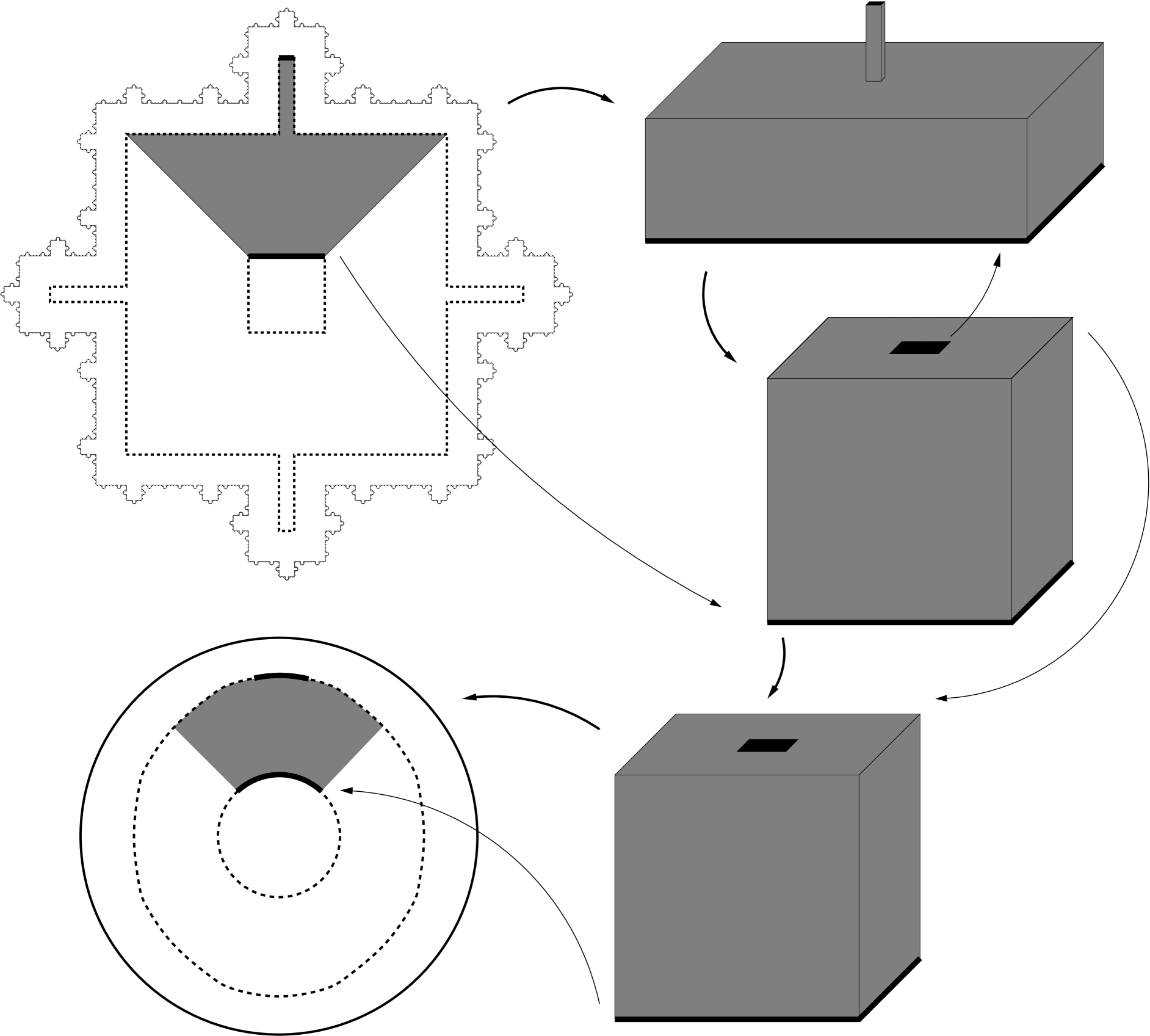
Figure 8. Construction of the extension $f$.

5.2. The Surfaces $\mathcal{R}_{j}$.

It will be convenient to consider distances with respect to the maximum norm in $\mathbb{R}^{3}$. These will be denoted by an $\infty$-subscript, i.e., we write

$$\operatorname{dist}_{\infty}(A,B):=\inf\{\|a-b\|_{\infty}:a\in A,b\in B\}.$$

In the same way we denote by $\operatorname{Hdist}_{\infty}$ the Hausdorff distance with respect to the maximum norm.

For a polyhedral surface $\mathcal{S}_{j}\subset\mathbb{R}^{3}$ homeomorphic to the sphere $\mathbb{S}$, let

(5.2) $$\operatorname{Interior}(\mathcal{S}_{j}):=\text{ bounded component of }\mathbb{R}^{3}\setminus\mathcal{S}_{j}.$$

Recall from Subsection 2.3 that the height of one face $\mathcal{T}$ of the snowball is at most $\frac{1}{2}-\frac{1}{N_{\max}}$. We approximate the snowsphere from the interior by the surfaces

(5.3) $$\mathcal{R}_{j}:=\left\{x\in\operatorname{Interior}(\mathcal{S}_{j}):\operatorname{dist}_{\infty}(x,\mathcal{S}_{j})=c\delta_{j}\right\},$$

where

$$c:=\left(\frac{1}{2}-\frac{1}{2N_{\max}}\right).$$

We chose the maximum norm in the definition of $\mathcal{R}_{j}$ to again get a polyhedral surface. Had we used the Euclidean distance instead, $\mathcal{R}_{j}$ would have some spherical pieces. Note that $c=\frac{1}{2}-\frac{1}{2N_{\max}}=(N_{\max}-1)\frac{1}{2N_{\max}}$. Consider one $\delta_{j}$-square $Q\subset\mathcal{S}_{j}$. Then the set $\{x\in\mathbb{R}^{3}:\operatorname{dist}_{\infty}(x,Q)\geq c\delta_{j}\}$ lives in the grid $\delta_{j}\frac{1}{2N_{\max}}\mathbb{Z}^{3}$. We conclude that

$$\text{the surface }\mathcal{R}_{j}\text{ lives in the grid }\delta_{j}\frac{1}{2N_{\max}}\mathbb{Z}^{3}.$$

In particular $\mathcal{R}_{j}$ is again a polyhedral surface.

Figure 9. $\mathcal{R}_{0},\mathcal{R}_{1},\mathcal{R}_{2}$ and $\mathcal{S}_{0},\mathcal{S}_{1},\mathcal{S}_{2}$.

Figure 9 shows a $2$-dimensional picture (the intersection with the plane $y=\frac{1}{2}$) of $\mathcal{R}_{0},\mathcal{R}_{1},\mathcal{R}_{2}$ (dashed line) and $\mathcal{S}_{0},\mathcal{S}_{1},\mathcal{S}_{2}$ (solid line) for the standard example $\widehat{\mathcal{S}}$ of Subsection 2.5.

We give a more detailed outline of the following subsections:

• In the next subsection we will see that the surfaces $\mathcal{R}_{j}$ “look combinatorially” like $\mathcal{S}_{j}$. More precisely, we will define a bijective projection $\pi_{j}\colon\mathcal{S}_{j}\to\mathcal{R}_{j}$, so the decomposition of $\mathcal{S}_{j}$ into $\delta_{j}$-squares is carried to $\mathcal{R}_{j}$. This shows that the surfaces $\mathcal{R}_{j}$ are topological spheres.

• In Subsection 5.4 we show that $\mathcal{R}_{j}$ and $\mathcal{R}_{j+1}$ are roughly parallel. This enables us to decompose the snowball $\mathcal{B}$ into shells, which are bounded by these surfaces.

• Such a shell is then (Subsection 5.5) decomposed into pieces. Up to scaling there are only finitely many different such pieces that occur.

We orient the approximations $\mathcal{S}_{j}$ by the normal pointing to the unbounded component of $\mathbb{R}^{3}\setminus\mathcal{S}_{j}$. Thus each $\delta_{j}$-square $Q$ from which $\mathcal{S}_{j}$ is built obtains an orientation. The two parts of the double pyramid of $Q$ are called outer and inner pyramids of $Q$ accordingly. To facilitate the discussion we will often map a $\delta_{j}$-square to the unit square $[0,1]^{2}\subset\mathbb{R}^{3}$ by an (orientation preserving) similarity, where the inner pyramid is mapped to $\mathcal{P}^{+}$, the one with tip $(\frac{1}{2},\frac{1}{2},\frac{1}{2})$ (and the tip of the outer one to $(\frac{1}{2},\frac{1}{2},-\frac{1}{2})$). It amounts to setting $\delta_{j}=1$. This normalizing map (defined on all of $\mathbb{R}^{3}$) is denoted by $\Phi=\Phi_{Q}$. It maps other $\delta_{j}$-squares to unit squares in $\mathbb{Z}^{3}$. Let $\Phi(\mathcal{R}_{j}):=\mathcal{R}$. We will often say that we work in the normalized picture, meaning that the local geometry around $Q$ ($\mathcal{S}_{j},\mathcal{R}_{j}$, and so on) was mapped by $\Phi$.

5.3. The $\mathcal{R}_{j}$ are topological Spheres

Here we define a bijective projection

(5.4) $$\pi_{j}\colon\mathcal{S}_{j}\to\mathcal{R}_{j}.$$

We will define $\pi_{j}$ as a map later (see the Remark on page Remark). For now we only have need for the following. We will define $\pi_{j}$ on the $1$-skeleton of $\mathcal{S}_{j}\,$, as well as define $\pi_{j}(Q)$ as a set, for any $\delta_{j}$-square $Q\subset\mathcal{S}_{j}$. The construction will be done locally, meaning we consider one such $\delta_{j}$-square $Q$ at a time.

Assume first that $\mathcal{S}_{j}$ is flat at $Q$, meaning all $\delta_{j}$-squares $Q^{\prime}\subset\mathcal{S}_{j}$ intersecting $Q$ are parallel. In the normalized picture let

(5.5) $$\pi(x_{1},x_{2},0):=(x_{1},x_{2},c)$$

be the projection of $[0,1]^{2}$ to $\mathcal{R}$. Then $\pi_{j}|_{Q}=\Phi_{Q}^{-1}\circ\pi\circ\Phi_{Q}$.

To define $\pi_{j}$ in general first consider a $\delta_{j}$-vertex $v$ of $\mathcal{S}_{j}$ ($v\in\mathcal{S}_{j}\cap\delta_{j}\mathbb{Z}^{3}$). At $v$ several $\delta_{j}$-squares from which $\mathcal{S}_{j}$ is built intersect. The projection of $v$ onto $\mathcal{R}_{j}$ is indicated in Figure 10. Here all possibilities (up to rotations/reflections) of how $\delta_{j}$-squares (drawn in white) can intersect in $v$ are shown. The shaded surfaces are the corresponding surfaces $\mathcal{R}_{j}$. The large dot shows the projection of $v$ onto $\mathcal{R}_{j}$. The formal (somewhat cumbersome) definition is as follows.

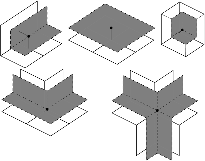
Figure 10. Projections of $v$ onto $\mathcal{R}_{j}$.

Let $\deg_{j}(v)$ be the number of $\delta_{j}$-squares of $\mathcal{S}_{j}$ intersecting in $v$. Two such $\delta_{j}$-squares are neighbors if they share an edge (of size $\delta_{j}$). We have to consider the case when $\deg_{j}(v)=5$ separately. So assume now that $\deg_{j}(v)=3,4,$ or $6$. Consider the planes through the intersecting edges bisecting the angle between neighbors. The intersection of all these planes and $\mathcal{R}_{j}$ is exactly one point $p=:\pi_{j}(v)$ such that $\lVert p-v\rVert_{\infty}=c\delta_{j}$.

Consider now the case $\deg_{j}(v)=5$. Note that the planes as above do not intersect $\mathcal{R}_{j}$ in a single point. Neighbors are either parallel or perpendicular. Consider only the planes through edges of perpendicular neighbors, bisecting their angle. The intersection of all these planes and $\mathcal{R}_{j}$ is exactly one point $p=:\pi_{j}(v)$ such that $\lVert p-v\rVert_{\infty}=c\delta_{j}$.

This defines $\pi_{j}$ for all vertices $v$ of $\mathcal{S}_{j}$. Let us record the properties:

• $\lVert v-\pi_{j}(v)\rVert_{\infty}=c\delta_{j}$.

• Let $v$ be a vertex of a $\delta_{j}$-square $Q\subset\mathcal{S}_{j}$, and let $\pi_{j}(v)$ be the projection onto $\mathcal{R}_{j}$. In the normalized picture (where $v$ mapped to the origin) the possible $x$- and $y$-coordinates of the projection are $c,0,-c$ (the $z$-coordinate is always $c$).

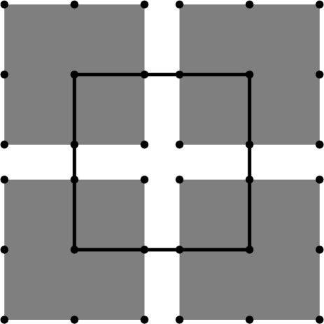
Figure 11. Possibilities of $\pi_{j}(v)$.

There are nine different possibilities for $\pi_{j}(v)$. Figure 11 shows these possibilities for the $4$ vertices of a square. Note that projections of different points lie in disjoint squares. The distance of the squares is given by the following. Consider two different $\delta_{j}$-vertices $v,v^{\prime}\in\mathcal{S}_{j}$. Then

$$\lVert\pi_{j}(v)-\pi_{j}(v^{\prime})\rVert_{\infty}\geq \lVert v-v^{\prime}\rVert_{\infty}-\lVert v-\pi_{j}(v)\rVert_{\infty}-\lVert v^{\prime}-\pi_{j}(v^{\prime})\rVert_{\infty}$$

$$\geq\delta_{j}-2c\delta_{j}=\frac{1}{N_{\max}}\delta_{j}.$$

Remark.

If at vertex $v\in\mathcal{S}_{j}$ the $\delta_{j}$-squares intersect as in the forbidden configuration (see Figure 2), the surface $\mathcal{R}_{j}$ has two corners corresponding to $v$. Exclusion of this case thus simplifies the decomposition considerably.

Let $E$ be an edge of a $\delta_{j}$-square $Q\subset\mathcal{S}_{j}$ with vertices $v,v^{\prime}$. Map $E$ affinely to the line segment with endpoints $\pi_{j}(v)$ and $\pi_{j}(v^{\prime})$. This defines $\pi_{j}$ on $E$, thus on the $1$-skeleton of $\mathcal{S}_{j}$.

Given a $\delta_{j}$-square $Q\subset\mathcal{S}_{j}$ with vertices $v_{1},v_{2},v_{3},v_{4}$, the projection $\pi_{j}(Q)\subset\mathcal{R}_{j}$ will be the quadrilateral with vertices $\pi_{j}(v_{k})$. It will in general not be a rectangle, in fact not even convex. Note also that we did not yet specify how individual points of $Q$ get mapped by $\pi_{j}$.

Lemma 5.1.

The projections $\pi_{j}$ satisfy the following:

1. For every $\delta_{j}$-square $Q\subset\mathcal{S}_{j}$, we have

   $$\operatorname{dist}_{\infty}(Q,\pi_{j}(Q))=\operatorname{Hdist}_{\infty}(Q,\pi_{j}(Q))=c\delta_{j}.$$

2. Consider the sets

   $$R_{j}:=\pi_{j}(Q),$$

   where $Q$ is a $\delta_{j}$-square in the approximation $\mathcal{S}_{j}$. These sets form a decomposition of the surface $\mathcal{R}_{j}$ into quadrilaterals, $\mathcal{R}_{j}=\bigcup R_{j}$. View $\mathcal{R}_{j}$ as a cell complex, where images of $\delta_{j}$-squares/edges/vertices by $\pi_{j}$ are the $2$-,$1$-, and $0$-cells. Then $\mathcal{R}_{j}$ and $\mathcal{S}_{j}$ are isomorphic as cell complexes.

3. The set $\mathcal{R}_{j}$ is a polyhedral surface homeomorphic to the unit sphere $\mathbb{S}$.

4. $\operatorname{Interior}(\mathcal{R}_{j})=\{x\in\operatorname{Interior}(\mathcal{S}_{j}):\operatorname{dist}_{\infty}(x,\mathcal{S}_{j})>c\delta_{j}\}$.

Proof.

To see (1) work in the normalized picture. Let $\pi\colon[0,1]^{2}\to\{z=c\}$ be the map conjugate to $\pi_{j}$ under the normalizing map $\Phi$. Then

$$Q_{*}:=[c,1-c]^{2}\times\{c\}\subset\pi([0,1]^{2})\subset[-c,1+c]^{2}\times\{c\}=:Q^{*};$$

see Figure 11, and Figure 12. Note that

$$c =\operatorname{dist}_{\infty}([0,1]^{2},Q_{*})=\operatorname{Hdist}_{\infty}([0,1]^{2},Q_{*})$$

$$=\operatorname{dist}_{\infty}([0,1]^{2},Q^{*})=\operatorname{Hdist}_{\infty}([0,1]^{2},Q^{*}).$$

The statement follows.

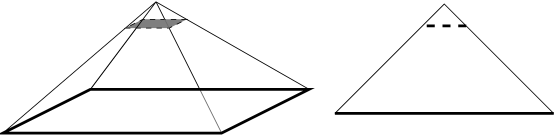
Figure 12. Part of $\mathcal{R}_{j}$.

Property (2) is clear from the construction.

Any homeomorphism $\pi_{j}\colon Q\to\pi_{j}(Q)$, that extends $\pi_{j}|_{\partial Q}$ yields Property (3).

(4) The set $\operatorname{Interior}(\mathcal{S}_{j})\setminus\mathcal{R}_{j}$ has two components by the PL-Schönflies theorem. The sets $\{x\in\operatorname{Interior}(\mathcal{S}_{j}):\operatorname{dist}_{\infty}(x,\mathcal{S}_{j})<c\delta_{j}\},\{x\in\operatorname{Interior}(\mathcal{S}_{j}):\operatorname{dist}_{\infty}(x,\mathcal{S}_{j})>c\delta_{j}\}$ are both non-empty (see Figure 12); pick points in the pyramid $\mathcal{P}^{+}$ above and below $Q_{*}$. Thus these sets are the two components. The statement follows from using PL-Schönflies again. ∎

Applying the same reasoning to the unbounded component of $\mathbb{R}^{3}\setminus\mathcal{S}_{j}$ yields the following.

Corollary 5.2.

The set $\{\operatorname{dist}_{\infty}(x,\mathcal{S}_{j})>c\delta_{j}\}$ has two components, one bounded (by $\mathcal{R}_{j}$) and one unbounded.

5.4. The shells between $\mathcal{R}_{j}$ and $\mathcal{R}_{j+1}$

We will show that the surfaces $\mathcal{R}_{j}$ and $\mathcal{R}_{j+1}$ are roughly parallel. This will enable us to decompose the snowball into shells bounded by two such surfaces.

Lower bounds on the distance will be controlled by $\operatorname{dist}_{\infty}$, while upper bounds of their distance will be controlled by the Hausdorff distance $\operatorname{Hdist}_{\infty}$. Note that $\operatorname{dist}_{\infty}$ is not suited to control upper bounds and that $\operatorname{Hdist}_{\infty}$ is not suited to control lower bounds on the distance.

Two sets $A$ and $B$ are called roughly $\delta$-parallel ($\delta>0$) with constant $C>0$ if

(5.6) $$\operatorname{dist}_{\infty}(A,B)\geq\frac{1}{C}\delta\;\mbox{ and }\operatorname{Hdist}_{\infty}(A,B)\leq C\delta.$$

Lemma 5.3.

The surfaces $\mathcal{S},\mathcal{S}_{j},$ and $\mathcal{R}_{j}$ satisfy

1. $\operatorname{Hdist}_{\infty}(\mathcal{R}_{j},\mathcal{S}_{j})=c\delta_{j}$.
   So $\mathcal{R}_{j}$ and $\mathcal{S}_{j}$ are (roughly) $c\delta_{j}$-parallel with constant $C=1$.

2. $\mathcal{R}_{j}$ and $\mathcal{S}$ are roughly $\delta_{j}$-parallel with constant $C=C(N_{\max})$ (independent of $j$).

3. $\operatorname{Interior}(\mathcal{R}_{j})$ is compactly contained in $\operatorname{Interior}(\mathcal{R}_{j+1})$, i.e.,

   $$\operatorname{Interior}(\mathcal{R}_{0})\Subset\operatorname{Interior}(\mathcal{R}_{1})\Subset\operatorname{Interior}(\mathcal{R}_{2})\Subset\dots\;.$$

4. $\mathcal{R}_{j}$ and $\mathcal{R}_{j+1}$ are roughly $\delta_{j}$-parallel with constant $C=C(N_{\max})$.

5. There is a positive integer $k_{0}$ such that

   $$\{\operatorname{dist}_{\infty}(x,\mathcal{S})>\delta_{j-k_{0}}\}\subset\{\operatorname{dist}_{\infty}(x,\mathcal{R}_{j})>c\delta_{j}\}\subset\{\operatorname{dist}_{\infty}(x,\mathcal{S})>\delta_{j+k_{0}}\},$$

   for all $j\geq k_{0}$.

Proof.

(1) Obviously

$$d_{\mathcal{S}_{j}}(\mathcal{R}_{j})=c\delta_{j};$$

this distance (see (1.2)) is again taken with respect to $\lVert\cdot\rVert_{\infty}$.

It remains to show that $d_{\mathcal{R}_{j}}(\mathcal{S}_{j})\leq c\delta_{j}$. Work again in the normalized picture. As before $Q_{*}=\{z=c\}\cap\mathcal{P}^{+}=[c,1-c]^{2}\times\{c\}\subset\mathcal{R}$; see Figure 12. Since $d_{Q_{*}}([0,1]^{2})=c$ it follows that $d_{\mathcal{R}_{j}}(\mathcal{S}_{j})\leq c\delta_{j}$.

(2) For every $x\in\mathcal{R}_{j}$ we have by (1.5)

$$\operatorname{dist}_{\infty}(x,\mathcal{S}) \geq\operatorname{dist}_{\infty}(x,\mathcal{S}_{j})-\operatorname{Hdist}_{\infty}(\mathcal{S}_{j},\mathcal{S})$$

$$\geq\left(\frac{1}{2}-\frac{1}{2N_{\max}}\right)\delta_{j}-\left(\frac{1}{2}-\frac{1}{N_{\max}}\right)\delta_{j}\mbox{, \quad by \eqref{eq:dSjS}}$$

$$=\frac{1}{2N_{\max}}\delta_{j}.$$

So $\operatorname{dist}_{\infty}(\mathcal{R}_{j},\mathcal{S})\geq\frac{1}{2N_{\max}}\delta_{j}$. Here we see that $c>\left(\frac{1}{2}-\frac{1}{N_{\max}}\right)$ ensures that $\mathcal{R}_{j}$ does not intersect the snowsphere $\mathcal{S}$.

On the other hand,

$$\operatorname{Hdist}_{\infty}(\mathcal{R}_{j},\mathcal{S}) \leq\operatorname{Hdist}_{\infty}(\mathcal{R}_{j},\mathcal{S}_{j})+\operatorname{Hdist}_{\infty}(\mathcal{S}_{j},\mathcal{S})$$

(5.7) $$\leq c\delta_{j}+\left(\frac{1}{2}-\frac{1}{N_{\max}}\right)\delta_{j}\leq\left(1-\frac{1}{N_{\max}}\right)\delta_{j}$$

(5.8) $$\leq\delta_{j},$$

by property (1) and (2.4).

(3) Consider an $x\in\mathbb{R}^{3}$ such that $\operatorname{dist}_{\infty}(x,\mathcal{S}_{j})\geq c\delta_{j}$. Then

$$\operatorname{dist}_{\infty}(x,\mathcal{S}_{j+1}) -c\delta_{j+1}$$

$$\geq \operatorname{dist}_{\infty}(x,\mathcal{S}_{j})-\operatorname{Hdist}_{\infty}(\mathcal{S}_{j},\mathcal{S}_{j+1})-c\delta_{j+1}$$

$$\geq c\delta_{j}-\left(\frac{1}{2}-\frac{3}{2}\frac{1}{N_{j+1}}\right)\delta_{j}-c\delta_{j+1},\quad\text{ by (\ref{eq:HdistSj})}$$

$$= \left[\frac{1}{2}-\frac{1}{2N_{\max}}-\frac{1}{2}+\frac{3}{2}\frac{1}{N_{j+1}}-\left(\frac{1}{2}-\frac{1}{2N_{\max}}\right)\frac{1}{N_{j+1}}\right]\delta_{j}$$

$$\geq \frac{1}{2N_{\max}}\delta_{j}.$$

Thus $\operatorname{dist}_{\infty}(x,\mathcal{S}_{j+1})>c\delta_{j+1}$, and hence

$$\{\operatorname{dist}_{\infty}(x,\mathcal{S}_{0})>c\delta_{0}\}\Subset\{\operatorname{dist}_{\infty}(x,\mathcal{S}_{1})>c\delta_{1}\}\Subset\dots\;.$$

The statement follows from Corollary 5.2 and Lemma 5.1 (4).

(4) One inequality follows immediately from inequality (5.8):

$$\operatorname{Hdist}_{\infty}(\mathcal{R}_{j},\mathcal{R}_{j+1}) \leq\operatorname{Hdist}_{\infty}(\mathcal{R}_{j},\mathcal{S})+\operatorname{Hdist}_{\infty}(\mathcal{S},\mathcal{R}_{j+1})$$

$$\leq\delta_{j}+\delta_{j+1}\leq 2\delta_{j}.$$

To see the second inequality recall inequality (2.3). Together with property (1) this yields

$$\begin{split}\operatorname{dist}_{\infty}(\mathcal{R}_{j},\mathcal{R}_{j+1})&\geq\operatorname{dist}_{\infty}(\mathcal{R}_{j},\mathcal{S}_{j})-\operatorname{Hdist}_{\infty}(\mathcal{S}_{j},\mathcal{S}_{j+1})-\operatorname{Hdist}_{\infty}(\mathcal{S}_{j+1},\mathcal{R}_{j+1})\end{split}$$

$$\begin{split}&\geq\left(\frac{1}{2}-\frac{1}{2N_{\max}}\right)\delta_{j}-\left(\frac{1}{2}-\frac{3}{2N_{j+1}}\right)\delta_{j}\\ &\phantom{XXXXXXXX}-\left(\frac{1}{2}-\frac{1}{2N_{\max}}\right)\delta_{j}\frac{1}{N_{j+1}}\end{split}$$

$$\geq\left(\frac{1}{N_{j+1}}-\frac{1}{2N_{\max}}\right)\delta_{j}\geq\frac{1}{2N_{\max}}\delta_{j}.$$

(5) Pick an $x\in\mathbb{R}^{3}$ such that $\operatorname{dist}_{\infty}(x,\mathcal{R}_{j})>\delta_{j}$. Then

$$\operatorname{dist}_{\infty}(x,\mathcal{S}) \geq\operatorname{dist}_{\infty}(x,\mathcal{R}_{j})-\operatorname{Hdist}_{\infty}(\mathcal{R}_{j},\mathcal{S})$$

$$>\delta_{j}-\left(1-\frac{1}{N_{\max}}\right)\delta_{j}\text{ by (\ref{eq:dRjSvar})}$$

$$=\frac{1}{N_{\max}}\delta_{j}.$$

Now pick $y\in\mathbb{R}^{3}$ with $\operatorname{dist}_{\infty}(y,\mathcal{S})>\delta_{j}$. Then

$$\operatorname{dist}_{\infty}(y,\mathcal{R}_{j}) \geq\operatorname{dist}_{\infty}(y,\mathcal{S})-\operatorname{Hdist}_{\infty}(\mathcal{S},\mathcal{R}_{j})$$

$$>\delta_{j}-\left(1-\frac{1}{N_{\max}}\right)\delta_{j}\text{ by (\ref{eq:dRjSvar})}$$

$$=\frac{1}{N_{\max}}\delta_{j}.$$

Choose $j_{0}$ such that $2^{j_{0}}\geq N_{\max}$. Thus

(5.9) $$\{\operatorname{dist}_{\infty}(x,\mathcal{S})>\delta_{j-j_{0}}\}\subset\{\operatorname{dist}_{\infty}(x,\mathcal{R}_{j})>\delta_{j}\}\subset\{\operatorname{dist}_{\infty}(x,\mathcal{S})>\delta_{j+j_{0}}\},$$

for all $j\geq j_{0}$. Note that $N_{\max}\geq 2$ implies

$$\frac{1}{2}>c=\frac{1}{2}-\frac{1}{2N_{\max}}\geq\frac{1}{4}.$$

Thus $\delta_{j+2}\leq c\delta_{j}<\delta_{j}$ and

(5.10) $$\{\operatorname{dist}_{\infty}(x,\mathcal{R}_{j})>\delta_{j}\}\subset\{\operatorname{dist}_{\infty}(x,\mathcal{R}_{j})>c\delta_{j}\}\subset\{\operatorname{dist}_{\infty}(x,\mathcal{R}_{j})>\delta_{j+2}\}.$$

The statement follows by combining (5.9) and (5.10) with $k_{0}=j_{0}+2$.

∎

By Property (3) of the last lemma we can define for $j\geq 0$ the shells

$$\mathcal{B}_{j}:=\operatorname{clos}\operatorname{Interior}(\mathcal{R}_{j+1})\setminus\operatorname{Interior}(\mathcal{R}_{j}),$$

bounded by $\mathcal{R}_{j}$ and $\mathcal{R}_{j+1}$. Property (4) of the previous lemma controls the “thickness” of these shells. By Property (5) and Corollary 5.2 we obtain the following.

Corollary 5.4.

The bounded component of $\mathbb{R}^{3}\setminus\mathcal{S}$ is

$$\bigcup_{j}\operatorname{Interior}(\mathcal{R}_{j})=\bigcup_{j}\mathcal{B}_{j}\cup\operatorname{Interior}(\mathcal{R}_{0})=\operatorname{int}\mathcal{B}.$$

It is simply connected, since each set $\operatorname{Interior}(\mathcal{R}_{j})$ is (using Lemma 5.3 (3)). Furthermore $\partial\mathcal{B}=\mathcal{S}$.

5.5. Decomposing the Shells

We decompose the shells $\mathcal{B}_{j}$ into pieces. This is the trickiest part of this section.

Fix a $\delta_{j}$-square $Q\subset\mathcal{S}_{j}$. We want to define a set $B(Q)\subset\mathcal{B}_{j}$ “above” $Q$. Work in the normalized picture. Let $\mathcal{R},\mathcal{R}^{\prime}$ be the images of $\mathcal{R}_{j},\mathcal{R}_{j+1}$ under the normalization. The piece of $\mathcal{S}_{j+1}$ bounded by $\partial Q$ maps (under the normalization) to $G$, which is the (correctly oriented) $N_{j+1}$-generator. It is built from squares of side-length $\delta:=1/N_{j+1}$. Call $\pi\colon[0,1]^{2}\to\mathcal{R}$ the map which is conjugate to $\pi_{j}\colon\mathcal{S}_{j}\to\mathcal{R}_{j}$ (under the normalization), and $\pi^{\prime}\colon G\to\mathcal{R}^{\prime}$ the one that is conjugate to $\pi_{j+1}\colon\mathcal{S}_{j+1}\to\mathcal{R}_{j+1}$. Note that we will only use $\pi,\pi^{\prime}$ as maps on $\partial[0,1]^{2}$ and $\pi([0,1]^{2}),\pi^{\prime}([0,1]^{2})$ as sets.

Assume first that all $\delta_{j}$-squares $Q^{\prime}\subset\mathcal{S}_{j}$ intersecting $Q$ are parallel to $Q$. Then $\pi^{\prime}(G)$ is a polyhedral surface bounded by $\partial[0,1]^{2}\times\{\delta c\}$. Also $\pi([0,1]^{2})=[0,1]^{2}\times\{c\}$. Note that by Lemma 5.3 (4) $\pi([0,1]^{2})\cap\pi^{\prime}(G)=\emptyset$. Consider a $\delta$-vertex $v$ in the interior of $G$, i.e., $v\in\delta\mathbb{Z}^{3}\cap G\setminus\partial[0,1]^{2}$. Then $\operatorname{dist}_{\infty}(v,\partial\mathcal{P})\geq\frac{1}{2}\delta$, here $\mathcal{P}$ denotes the double pyramid (see Section 2.1, and Figure 3). Thus

(5.11) $$\operatorname{dist}_{\infty}(\pi^{\prime}(v),\partial\mathcal{P}) \geq\operatorname{dist}_{\infty}(v,\partial\mathcal{P})-\lVert v-\pi^{\prime}(v)\rVert_{\infty}$$

$$\geq\frac{1}{2}\delta-c\delta=\frac{1}{2N_{\max}}\delta,$$ by Subsection 5.3.

Thus $\pi^{\prime}(G)\cup\left([0,1]^{2}\times\{c\}\right)\cup\left(\partial[0,1]^{2}\times[c\delta,c]\right)$ is a polyhedral surface homeomorphic to the sphere $\mathbb{S}$.

Using the PL-Schönflies theorem in $\mathbb{R}^{3}$ once more, we define the standard piece corresponding to the generator $G$ (with given orientation) as the set

(5.12) $$B_{G} =B_{G}([0,1]^{2})$$

$$:=\operatorname{clos}\operatorname{Interior}\pi^{\prime}(G)\cup\left([0,1]^{2}\times\{c\}\right)\cup\left(\partial[0,1]^{2}\times[c\delta,c]\right).$$

See Figure 13 for a two-dimensional picture. The piece $B(Q)$ will be the image of $B_{G}([0,1]^{2})$ under (the inverse of) the normalizing map, where $G=G_{j}$ is the (correctly oriented) generator by which $Q$ was replaced to construct $\mathcal{S}_{j+1}$.

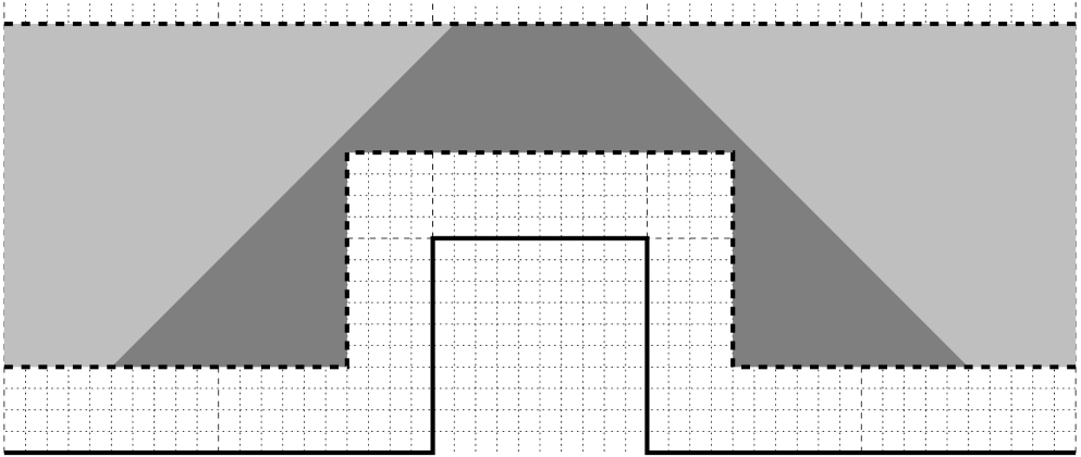
Figure 13. The standard piece $B_{G}$.

Let the $\delta_{j}$-square $Q\subset\mathcal{S}_{j}$ be arbitrary. To define the piece $B(Q)\subset\mathcal{B}_{j}$ we again work first in the normalized picture.

Definition 5.5.

The set $B$ is the one bounded by $\pi([0,1]^{2}),\pi^{\prime}(G)$ and the line segments with endpoints $\pi(v),\pi^{\prime}(v)$ for all $v\in\partial[0,1]^{2}$.

Call $\pi([0,1]^{2})$ the inner side and $\pi^{\prime}(G)$ the outer side of $B$; the outer side is closer to $\mathcal{S}$ than the inner side. We will show that $B$ is bi-Lipschitz to the standard piece $B_{G}$ (5.12).

The following discussion can be paraphrased in the following way: The piece $B$ has a “core” which is identical to the one of $B_{G}$. The “rest” of $B$ has “trivial geometry” (not depending on the generator $G$), which can be used to deform $B$ into $B_{G}$.

Consider a $\delta$-square $Q^{\prime}\subset G$. It will be called an interior square if $Q^{\prime}\cap\partial[0,1]^{2}=\emptyset$ and a boundary square otherwise. From (5.11) we obtain $\operatorname{dist}_{\infty}(Q^{\prime},\partial\mathcal{P})\geq\frac{1}{2N_{\max}}$ for such an interior $\delta$-square $Q^{\prime}\subset G$. Note that each boundary $\delta$-square $Q^{\prime}\subset G$ lies in the $xy$-plane. Define

$$\operatorname{core}(B):=\left\{x\in B:\operatorname{dist}_{\infty}(x,\partial\mathcal{P})\geq\frac{1}{4N_{\max}}\delta\right\}.$$

See Figure 13; here $\operatorname{core}(B_{G})$ is the darker shaded region. We map $\operatorname{core}(B)$ to $\operatorname{core}(B_{G})$ by the identity. The “remaining set” $B\setminus\operatorname{core}(B)$ can be broken up into pieces and mapped to the corresponding piece in $B_{G}$ using Lemma 4.2.

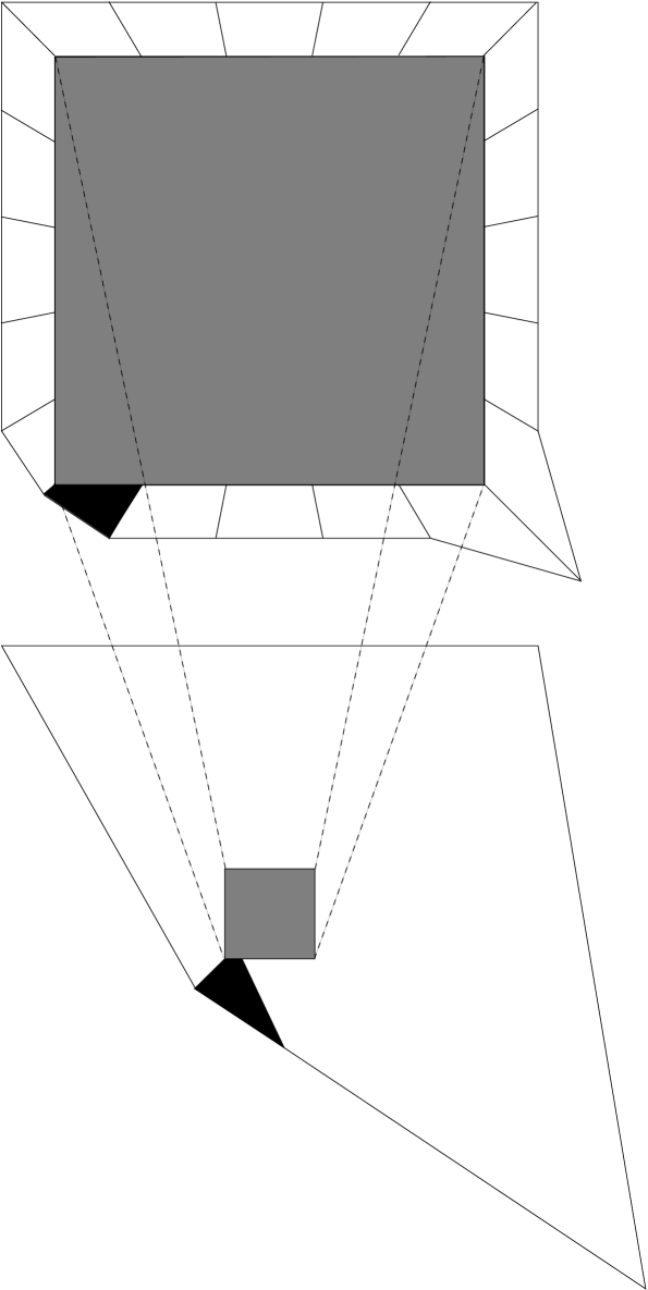
Figure 14. Decomposing $B\setminus\operatorname{core}(B)$.

For the reader who is a stickler we give a precise construction. It is illustrated in Figure 14. The outer side is shown on top, the inner side on the bottom. Thus the picture is “turned around” compared to Figure 13. The set $\operatorname{core}(B)$ is indicated as the shaded region. Note that this is not a situation occurring for our standard example $\widehat{\mathcal{S}}$. The picture is not to scale as well.

First consider the outer side of the remaining piece, i.e., the set $\mathcal{R}^{\prime}\cap(B\setminus\operatorname{core}(B))$. The set $\partial\operatorname{core}(B)\cap\mathcal{R}^{\prime}$ is a square, each side of which we decompose into $N_{j+1}$ line segments (of the same size). The other boundary component is $\pi^{\prime}(\partial G)=\pi^{\prime}(\partial[0,1]^{2})$. The images of the $\delta$-edges decompose it into $4N_{j+1}$ line segments. Connect corresponding line segments (by line segments) to obtain the decomposition of the outer side of $B\setminus\operatorname{core}(B)$ into quadrilaterals.

Now consider the inner side of the remaining piece, i.e., the set $\mathcal{R}\cap(B\setminus\operatorname{core}(B))$. It is bounded by a square ($\partial\operatorname{core}(B)\cap\mathcal{R}$) and the quadrilateral $\pi(\partial[0,1]^{2})$. Each side of the two quadrilaterals gets decomposed into $N_{j+1}$ pieces of the same length. Connecting corresponding edges in the two boundary components decomposes $\mathcal{R}\cap(B\setminus\operatorname{core}(B))$ into quadrilaterals. This is shown only for one quadrilateral in Figure 14.

The set $B\setminus\operatorname{core}(B)$ gets decomposed into pieces between corresponding quadrilaterals in the outer and inner face as in equation (4.7). Use the map from (4.8) to map corresponding pieces of $B\setminus\operatorname{core}(B)$ to $B_{G}\setminus\operatorname{core}(B_{G})$. Note that this piecewise defined map agrees on intersections. A tedious, but elementary computation shows that the maps do not degenerate, i.e., that (4.6) is satisfied.

As an example, we do the computation for the piece bounded by the black quadrilaterals indicated in Figure 14. The $xy$-coordinates of the vertices of the outer (black) quadrilateral (shown on top) are

$$P_{0}^{1} =\delta c\left<1,1\right>, P_{1}^{1}=\delta\left<1,0\right>,$$

$$P_{2}^{1} =\frac{1}{2}\delta\left<1,1\right>+\delta(1-\delta)\left<1,0\right>, P_{3}^{1}=\frac{1}{2}\delta\left<1,1\right>.$$

The ones for the inner (black) quadrilateral (shown at the bottom) are

$$P_{0}^{0} =c\left<1,1\right>,\phantom{XXXXXXXX}P_{1}^{0}=c\left<1,1\right>+\delta\left<1,-2c\right>,$$

$$P_{2}^{0} =\left(c+\frac{1}{2N_{\max}}\delta\right)\left<1,1\right>+\delta\frac{1}{N_{\max}}(1-\delta)\left<1,0\right>,$$

$$P_{3}^{0} =\left(c+\frac{1}{2N_{\max}}\delta\right)\left<1,1\right>.$$

Define $P_{k}^{u}:=(1-u)P_{k}^{0}+uP_{k}^{1},\;u\in[0,1]$, as in Section 4. For $J$ as in (4.6) one computes

$$J\geq\frac{\delta^{2}}{4N_{\max}^{2}}.$$

One checks the non-degeneracy (positivity of $J$) of other pieces and types of vertices by the same type of computation. In this fashion $B\setminus\operatorname{core}(B)$ is decomposed into sets bi-Lipschitz equivalent to the cube $[0,1]^{3}$. Map those to corresponding pieces in the standard piece. Note that the maps agree on intersecting faces by the construction of the maps from (4.8).

We have proved the following.

Lemma 5.6.

There is a bi-Lipschitz map

$$f_{1}=f_{1,B}\colon B\to B_{G}.$$

There are only finitely many different sets $B$ (and $B_{G}$). So we can assume that the maps $f_{1,B}$ have a common bi-Lipschitz constant $L$.

For a $\delta_{j}$-square $Q_{j}\subset\mathcal{S}_{j}$, now define the set $B(Q_{j})\subset\mathcal{B}_{j}$ as the inverse of the set $B$ (defined above) under the normalization.

Note that $[c,1-c]^{3}$ is bounded by $\mathcal{R}_{0}$.

Lemma 5.7.

The sets $B(Q_{j})$ together with the set $[c,1-c]^{3}$ form a Whitney-type decomposition of the snowball; this means

1. $$\bigcup_{\begin{subarray}{c}j\geq 0\\ Q_{j}\subset\mathcal{S}_{j}\end{subarray}}B(Q_{j})\cup[c,1-c]^{3}=\operatorname{int}\mathcal{B}.$$

2. The interiors of the sets $B(Q_{j})$ are pairwise disjoint.

3. $$\operatorname{diam}B(Q_{j})\asymp\operatorname{dist}(B(Q_{j}),\mathcal{S})\asymp\delta_{j},$$

   where $C(\asymp)=C(N_{\max})$.

Proof.

The first statement follows from Corollary 5.4. The second is clear from the construction. The third follows from Lemma 5.3 (2) and (4). ∎

The composition of the normalizing map and the one from Lemma 5.6 is still called

(5.13) $$f_{1}=f_{1,Q}\colon B(Q)\to B_{G}.$$

This map is quasisimilar (see (5.1)), where the scaling factor is $l=1/\delta_{j}$ and the constant $L$ is uniform. In Figure 8 this map, as well as the following ones, is illustrated.

Remark.

The map $f_{1}\colon B(Q)\to B_{G}$ can be used to define

(5.14) $$\pi_{j}\colon\mathcal{S}_{j}\to\mathcal{R}_{j}.$$

Namely, map $Q$ isometrically to $[0,1]^{2}\times\{c\}$, which in turn is mapped to $\pi_{j}(Q)\subset\mathcal{R}_{j}$ by $f_{1}^{-1}$. Formally $\pi_{j}|_{Q}:=f_{1}^{-1}\circ\pi\circ\Phi_{Q}$ ($\Phi_{Q}$ is the normalizing map, $\pi$ from equation (5.5)). The map $\Phi_{Q}$ has to be the same as the one used in the definition of $f_{1}$, so vertices are mapped correctly. Note that this definition agrees with the previous definition of $\pi_{j}$ on the $1$-skeleton of $\mathcal{S}_{j}$ (edges are mapped affinely). The maps $\pi_{j}$ are bi-Lipschitz with a common bi-Lipschitz constant $L$.

Consider two distinct $\delta_{j}$-squares $Q,Q^{*}\subset\mathcal{S}_{j}$. We think of $B_{G}(Q)=f_{1,Q}(B(Q))$ and $B_{G^{*}}(Q^{*})=f_{1,Q^{*}}(B(Q^{*}))$ as being distinct, since they are to be mapped to different sets. Note that $G,G^{*}$ are the same generators, but may have different orientation. There are only finitely many different sets $B_{G}(Q)$ throughout the construction, up to isometries.

Lemma 5.8.

The map $f_{1}$ is compatible on neighbors (i.e., $Q,Q^{*}$ intersecting in a $\delta_{j}$-edge). This means the following. Identify appropriate sides of $B_{G}(Q)$ and $B_{G^{*}}(Q^{*})$ (one of the four sides $\partial[0,1]^{2}\times[\frac{c}{N_{j+1}},c]$). Then $f_{1}=f_{1}^{*}$ on $B(Q)\cap B(Q^{*})$.

Proof.

Work again in the normalized picture. Consider a $v\in\partial[0,1]^{2}$. The boundary of $B$ contains the line segment with endpoints $\pi(v),\pi^{\prime}(v)$. The map $f_{1}$ maps this line segment affinely to $\{v\}\times[\frac{c}{N_{j+1}},c]$. The same is true for the map $f^{*}_{1}$ on the neighboring piece $B^{*}$. ∎

Consider (for a given generator) our standard piece $B_{G}$. Recall from Subsection 5.2 that $\mathcal{R}_{j}$ lives in the grid $\delta_{j}\frac{1}{2N_{\max}}\mathbb{Z}^{3}$. Thus $B_{G}$ lives in the grid $\frac{1}{2N_{j+1}N_{\max}}\mathbb{Z}^{3}$. This is indicated (for our standard example) in Figure 13. The boundary of $B_{G}$ consists of $[0,1]^{2}\times\{c\}$, $\pi^{\prime}(G)$, and four sides perpendicular to the $xy$-plane ($\partial[0,1]^{2}\times[\frac{c}{N_{j+1}},c]$).

Using Corollary 1.2 we can map $B_{G}$ orientation preserving to the unit cube by a bi-Lipschitz map

(5.15) $$f_{2}=f_{2,B_{G}}\colon B_{G}\to[0,1]^{3}.$$

We further require that $f_{2}$ maps

• $[0,1]^{2}\times\{c\}$ (the inner side) isometrically to $[0,1]^{2}\times\{0\}$;

• $\pi^{\prime}(G)$ (the outer side) to $[0,1]^{2}\times\{1\}$;

• the sides $\partial[0,1]^{2}\times[\frac{c}{N_{j+1}},c]$ affinely to $\partial[0,1]^{2}\times[0,1]$.

To see that we can make these further assumptions, either go through the proof of the PL-Schönflies theorem or post-compose with a map from Lemma 4.5.

As before we think of images of $f_{2}$ as distinct, i.e., $f_{2}(B_{G}(Q))=[0,1]^{3}=[0,1]^{3}(Q)$. Since there are only finitely many different sets $B_{G}$ (up to isometries), we can assume that all maps $f_{2}$ have a common bi-Lipschitz constant $L$.

It will be convenient to restrict our attention to the surfaces $\mathcal{R}_{j}$ (and their images). Recall the sets $R_{j}:=\pi_{j}(Q_{j})$ from the decomposition of the surfaces $\mathcal{R}_{j}$ (Lemma 5.1 (2)), where $Q_{j}\subset\mathcal{S}_{j}$ is a $\delta_{j}$-square. Define

(5.16) $$\phi_{R_{j}}\colon R_{j}\to[0,1]^{2}=[0,1]^{2}\times\{0\}\quad\text{ by }$$

$$\phi_{R_{j}}:=f_{2}\circ f_{1}|_{R_{j}},$$

where $f_{1}=f_{1,Q_{j}},f_{2}=f_{2,B_{G_{j}}}$; the inner side of the piece $B(Q_{j})$ is mapped here. The maps $\phi_{R_{j}}$ are quasisimilarities with scaling factor $l=1/\delta_{j}$ and uniform constant $L$. Again we think of the squares $[0,1]^{2}(R_{j}):=\phi_{R_{j}}(R_{j})$ as being distinct.

We now turn our attention to how the outer side of the piece $B(Q_{j})$ is mapped. Let $R_{j+1}$ be a set from the decomposition of $\mathcal{R}_{j+1}$ contained in (the outer side of) $B(Q_{j})$. Let

(5.17) $$T_{j+1}:=f_{2}\circ f_{1}(R_{j+1})\subset[0,1]^{2}\times\{1\},$$

where $f_{1}=f_{1,Q_{j}},f_{2}=f_{2,B_{G_{j}}}$ as before. All such sets decompose $[0,1]^{2}\times\{1\}$, the “top face” of the cube. To later be able to “put adjacent shells together” in a compatible way, we introduce the following maps:

(5.18) $$\psi_{T_{j+1}} \colon T_{j+1}\to[0,1]^{2}=[0,1]^{2}\times\{0\},\text{ defined by}$$

$$\psi_{T_{j+1}} :=\phi_{R_{j+1}}\circ f_{1}^{-1}\circ f_{2}^{-1}$$

on $T_{j+1}$. Note that in this expression $f_{1}=f_{1,Q_{j}},f_{2}=f_{2,B_{G_{j}}}$, and $\phi_{R_{j+1}}=f_{2,Q_{j+1}}\circ f_{1,B_{G_{j+1}}}$ ($R_{j+1}=\pi_{j+1}(Q_{j+1})$). This means we are comparing how $R_{j+1}$ is mapped as a set in the outer side of the piece $B(Q_{j})$ versus how it is mapped as the inner side of the piece $B(Q_{j+1})$. There are only finitely many different sets $T_{j+1}$, thus the maps $\psi_{T_{j+1}}$ have a common bi-Lipschitz constant $L$. Figure 8 again illustrates the map. Note however that the picture is incorrect insofar as $\psi_{T_{j+1}}$ maps between cubes $[0,1]^{3}(Q_{j}),[0,1]^{3}(Q_{j+1})$ coming from pieces in different shells $\mathcal{B}_{j},\mathcal{B}_{j+1}$.

Remark.

In the construction of the maps $f_{1}$ and $f_{2}$ the symmetry of the generators was not used. We merely used the facts that there are only finitely many different ones and that they fit inside the double pyramid.

Guide to notation.

We mapped pieces $B(Q)$ and quadrilaterals $R_{j}$ from the decomposition of the snowball $\mathcal{B}$ to “normalized” ones (cubes, squares). In the next section these cubes will be mapped into the unit ball $\mathbb{B}$. Maps $\mathcal{B}\to[0,1]^{3}$ are denoted by $\phi$. Maps $[0,1]^{3}\to\mathbb{B}$ will be denoted by $\varphi$. Intermediate maps $[0,1]^{3}\to[0,1]^{3}$ are denoted by $\psi$. Note that $\phi,\psi,\varphi$ are maps on surfaces, namely on $\mathcal{R}_{j}$ and images of them. Again the reader is advised to consult Figure 8.

6. Reassembling the Unit Ball

6.1. Conformal Triangles

Recall how in Subsection 3.2 uniformization of the $j$-th approximation $\mathcal{S}_{j}$ was used to decompose the sphere $\mathbb{S}=\{\lvert x\rvert=1\}$ conformally into $j$-tiles $X^{\prime}$

$$\mathbb{S}=\bigcup_{X^{\prime}\in\mathbf{X}^{\prime}_{j}}X^{\prime}.$$

Since it is easier to deal with simplices, we will decompose each conformal square $X^{\prime}$ into $4$ triangles. Divide the unit square $[0,1]^{2}$ along the diagonals into $4$ triangles and map them to $X^{\prime}\in\mathbf{X}^{\prime}_{j}$ by the conformal map $[0,1]^{2}\to X^{\prime}$ (normalized by mapping vertices to vertices).

Alternatively we could divide each $\delta_{j}$-square in the $j$-th approximation $\mathcal{S}_{j}$ along the diagonals into $4$ $\delta_{j}$-triangles and use uniformization on this polyhedral surface to get the decomposition of the sphere $\mathbb{S}$ into conformal $j$-triangles. Denote the set of these conformal $j$-triangles by $\widetilde{\mathbf{X}}_{j}$. Again $\widetilde{\mathbf{X}}_{j}$ forms a conformal tiling, i.e., every $\widetilde{X}\in\widetilde{\mathbf{X}}_{j}$ is a conformal reflection of its neighbors along shared sides. Figure 15 shows the conformal $1$-triangles of our main example $\widehat{\mathcal{S}}$. It is again conformally correct up to numerical errors. Compare this picture with Figure 6.

Each conformal $j$-triangle has edges and vertices via the conformal map. Again we speak of edges and vertices of order $j$ (or $j$-edges and $j$-vertices).

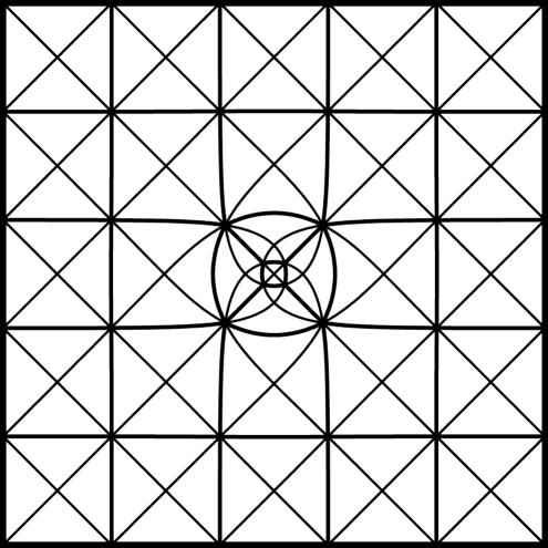
Figure 15. Conformal $1$-triangles of $\widehat{\mathcal{S}}$.

It is true that each conformal $(j+1)$-triangle is contained in exactly one conformal $j$-triangles. So the conformal $(j+1)$-triangles subdivide the conformal $j$-triangles. We do not need to prove this here.

Let $\widetilde{X}$ be a conformal $j$-triangle, $\widetilde{Y}\in\widetilde{\mathbf{X}}_{j}$ have non-empty intersection with $\widetilde{X}$, and $\widetilde{X}\subset X^{\prime}\in\mathbf{X}^{\prime}_{j}$ be the $j$-tile containing it. Then using the same argument as in Lemma 3.7

(6.1) $$\operatorname{diam}\widetilde{Y}\asymp\operatorname{diam}\widetilde{X}\asymp\operatorname{diam}X^{\prime}.$$

Here $C(\asymp)=C(N_{\max})$.

Map the triangulation of $\mathcal{S}_{j}$ by $\pi_{j}$ (5.14) to the surface $\mathcal{R}_{j}$; images of $\delta_{j}$-triangles are called $\widetilde{R}_{j}$. We have obtained a triangulation of $\mathcal{R}_{j}=\bigcup\widetilde{R}_{j}$. Each quadrilateral $R_{j}$ thus gets divided into $4$ sets $\widetilde{R}_{j}$.

Identify a quarter of the square $[0,1]^{2}$ with the standard $2$-simplex $\Delta$ (4.13); then $\phi_{R_{j}}(\widetilde{R}_{j})=\Delta=\Delta(\widetilde{R}_{j})$ (see (5.16) as well as the definition of $\pi_{j}$ (5.14)). We equip each such $2$-simplex with the metric $\lVert\cdot\rVert_{\Delta}$ from (4.14) (so they are all isometric).

Every set $\widetilde{R}_{j}$ gets mapped by $\pi_{j}^{-1}$ to a $\delta_{j}$-triangle in $\mathcal{S}_{j}$, which the uniformization maps to a conformal $j$-triangle $\widetilde{X}_{j}\subset\mathbb{S}$. We call $\widetilde{X}_{j}$ the conformal triangle corresponding to $\widetilde{R}_{j}$ and write $\widetilde{X}_{j}=\widetilde{X}_{j}(\widetilde{R}_{j})$. By the same procedure vertices and edges of $\widetilde{R}_{j}$ are mapped to the corresponding edges and vertices of $\widetilde{X}_{j}$.

Similarly every $R_{j}$ (from the decomposition of $\mathcal{R}_{j}$ in Lemma 5.1 (2)) is mapped by $\pi^{-1}_{j}$ to a $\delta_{j}$-square $Q_{j}\subset\mathcal{S}_{j}$, which in turn is mapped by the uniformization to the corresponding $j$-tile $X^{\prime}_{j}=X^{\prime}_{j}(R_{j})\in\mathbf{X}^{\prime}_{j}$.

6.2. Overview of the Decomposition of the unit Ball

Before getting into details let us give a brief overview of this section. We will decompose the open unit ball $\operatorname{int}\mathbb{B}=\{\lvert x\rvert<1\}$ into shells $\{\rho_{j}\leq\operatorname{dist}(x,\mathbb{S})\leq\rho_{j+1}\}$, which get decomposed into sets of the form

$$\{(\omega,\rho)\in\mathbb{S}\times[0,1]=\mathbb{B}:\omega\in X_{j}^{\prime},\;\rho_{j}\leq\rho\leq\rho_{j+1}\},$$

where $X_{j}^{\prime}\in\mathbf{X}^{\prime}_{j}$ (using spherical coordinates). We will map cubes (being images of the pieces $B(Q_{j})$) to these sets.

To assure quasiconformality we need $\operatorname{diam}X_{j}^{\prime}\!\asymp\rho_{j+1}-\rho_{j}$. Since $\operatorname{diam}X_{j}^{\prime}/\!\operatorname{diam}Y_{j}^{\prime}$ (where $X_{j}^{\prime},Y_{j}^{\prime}\in\mathbf{X}^{\prime}_{j}$) is neither bounded above nor below, radii will not be constant on $\mathbb{S}$, but rather we will have $\rho_{j}=\rho_{j}(\omega)$.

In the next subsection our main concern is that neighboring pieces $B(Q_{j})$ and $B(P_{j})$ (where the $\delta_{j}$-squares $Q_{j}$ and $P_{j}$ are neighbors) are mapped in a compatible way, i.e., the maps agree on the intersecting face.

In Subsection 6.4 we make sure that pieces “on top of each other” are mapped in a compatible way. More precisely, given a $\delta_{j}$-square $Q_{j}\subset\mathcal{S}_{j}$ and a $\delta_{j+1}$-square $Q_{j+1}\subset G(Q_{j})\subset\mathcal{S}_{j+1}$, we require that the maps on $B(Q_{j})$ and $B(Q_{j+1})$ agree on their intersection. Here $G(Q_{j})$ is the scaled generator replacing $Q_{j}$ in the construction of $\mathcal{S}_{j+1}$.

6.3. Constructing the Maps $\varphi_{\widetilde{X}}\colon\Delta\to\widetilde{X}$

First we will construct maps $\varphi_{\widetilde{X}}$ from the $2$-simplex $\Delta$ to a conformal $j$-triangle $\widetilde{X}$.

We could of course use the Riemann map for this. The downside is that this map will in general have singularities at the vertices, which would make the extension to the cube $[0,1]^{3}$ somewhat difficult (though most likely doable). We choose a different approach here; $\varphi_{\widetilde{X}}$ will be a quasisimilarity (see (5.1)) with scaling factor $l\asymp\operatorname{diam}\widetilde{X}$ and uniform constant $L$. This makes extension of the map easier. We have to make sure that the maps are compatible on neighbors $\widetilde{X},\widetilde{Y}\in\widetilde{\mathbf{X}}_{j}$. More precisely, if $\Delta^{\prime}$ is a reflection of $\Delta$ along one of its edges $E=\Delta\cap\Delta^{\prime}$ which is mapped to the common edge of $\widetilde{X}$ and $\widetilde{Y}$ by the maps $\varphi_{\widetilde{X}}\colon\Delta\to\widetilde{X}$ and $\varphi_{\widetilde{Y}}\colon\Delta^{\prime}\to\widetilde{Y}$

$$\varphi_{\widetilde{X}}(E)=\widetilde{X}\cap\widetilde{Y}=\varphi_{\widetilde{Y}}(E),$$

then

(6.2) $$\varphi_{\widetilde{X}}|_{E}=\varphi_{\widetilde{Y}}|_{E}.$$

If we used the Riemann maps for $\varphi_{\widetilde{X}}$ and $\varphi_{\widetilde{Y}}$ instead, this would follow immediately by the reflection principle.

Note that by construction the number of conformal $j$-triangles intersecting in a $j$-vertex is always even. Consider one such $j$-triangle $\widetilde{X}$. If at its vertices $2n$, $2m$, and $2l$ $j$-triangles intersect (in counterclockwise order), the angles are $\frac{\pi}{n}$, $\frac{\pi}{m}$, and $\frac{\pi}{l}$. We say $\widetilde{X}$ is of type $(n,m,l)$. Consider a neighborhood of $\widetilde{X}$

$$U(\widetilde{X}):=\operatorname{int}\>\bigcup\{\widetilde{Z}\in\widetilde{\mathbf{X}}_{j}:\widetilde{X}\cap\widetilde{Z}\neq\emptyset\}.$$

One can get $U(\widetilde{X})$ by repeated reflection. Therefore the Riemann map $\psi\colon\widetilde{X}\to\widetilde{Y}$ between two conformal triangles $\widetilde{X}$ and $\widetilde{Y}$ of the same type (normalized by mapping vertices to corresponding vertices) extends to these neighborhoods $\overline{\psi}\colon U(\widetilde{X})\to U(\widetilde{Y})$. Since $\widetilde{X}$ is compactly contained in $U(\widetilde{X})$, $\psi$ is quasisimilar by Koebe distortion. For each occurring type $(n,m,l)$ we fix one conformal triangle $X(n,m,l)$ of this type. There are only finitely many $X(n,m,l)$. We will now construct bi-Lipschitz maps

$$\varphi\colon\Delta\to X(n,m,l).$$

By composing with a Riemann map $\psi=\psi_{\widetilde{Y}}\colon X(n,m,l)\to\widetilde{Y}$ as above ($\widetilde{Y}$ is of type $(n,m,l)$), we get a quasisimilarity

(6.3) $$\varphi_{\widetilde{Y}}:=\psi\circ\varphi\colon\Delta\to\widetilde{Y}$$

for any conformal triangle $\widetilde{Y}$. The scaling factor of $\varphi_{\widetilde{Y}}$ is $l=|\psi^{\prime}(x)|\asymp\operatorname{diam}\widetilde{Y}$ for any $x\in X(n,m,l)$, and the bi-Lipschitz constant $L$ of $\varphi_{\widetilde{Y}}$ is uniform (by Koebe).

Initially the maps $\varphi$ will only be defined on the boundary $\partial\Delta$ of $\Delta$. In fact, let us first define $\varphi$ just on one edge of $\Delta$. For simplicity we assume this edge to be $[0,1]\subset\mathbb{R}^{2}$ and $\Delta\subset\mathbb{R}^{2}$. Now consider an edge $E^{\prime}\subset\partial\widetilde{X}$ of a conformal triangle $\widetilde{X}\in\widetilde{\mathbf{X}}_{j}$. We say $E^{\prime}$ is of type $(n,m)$ if $\widetilde{X}$ has angles $\frac{\pi}{n}$ and $\frac{\pi}{m}$ (in counterclockwise order as a boundary of $\widetilde{X}$) at the vertices of $E^{\prime}$. For an edge $E^{\prime}$ of order $j$ consider a neighborhood

$$U(E^{\prime}):=\operatorname{int}\>\bigcup\{\widetilde{Z}\in\widetilde{\mathbf{X}}_{j}:\widetilde{Z}\cap E^{\prime}\neq\emptyset\}.$$

Let $\widetilde{X}$ be a conformal triangle of type $(n,m,l)$ and $\widetilde{Y}$ one of type $(n,m,\tilde{l})$. Then the conformal map $\varphi\colon\widetilde{X}\to\widetilde{Y}$ (normalized by mapping $1$st, $2$nd, and $3$rd vertex onto each other) extends to a map $\overline{\varphi}\colon U(E^{\prime})\to U(F^{\prime})$, where $E^{\prime}\subset\partial\widetilde{X}$ and $F^{\prime}\subset\partial\widetilde{Y}$ are the edges of type $(n,m)$. So $\varphi$ is a quasisimilarity on $E^{\prime}$ by Koebe.

For each occurring type $(n,m)$ of an edge, we define $T(n,m)\subset\mathbb{R}^{2}$ to be a (fixed)

• circular arc triangle, meaning all its edges are circular arcs.

• One edge of $T(n,m)$ is $[0,1]\subset\mathbb{R}^{2}$, which is of type $(n,m)$. We think of $[0,1]$ as the image of the edge $[0,1]\subset\partial\Delta$ under the identity.

• $T(m,n)$ is the reflection of $T(n,m)$ along the line $x=\frac{1}{2}$. This means we can put $T(n,m)$ in the upper and $T(m,n)$ in the lower half plane, such that $T(m,n)=\overline{T(n,m)}$ ($\bar{z}$ denotes complex conjugation). In particular $T(n,n)$ is symmetric with respect to $x=\frac{1}{2}$.

The third angle of $T(n,m)$ is arbitrary. The third condition will ensure compatibility in the sense of equation (6.2), as will be seen in the next lemma. For the edge $E\subset X(n,m,l)$ of type $(n,m)$ we define the map $\varphi_{E}\colon[0,1]\to E$ by $\varphi_{E}:=\zeta|_{[0,1]}$, where $\zeta\colon T(n,m)\to X(n,m,l)$ is the Riemann map (normalized by mapping vertices to vertices, in particular vertices with angles $\frac{\pi}{n}$ and $\frac{\pi}{m}$ onto each other). By the above consideration $\varphi_{E}$ is bi-Lipschitz. Using the same procedure on the other edges we get a bi-Lipschitz map $\varphi\colon\partial\Delta\to\partial X(n,m,l)$ (here we are using the fact that $X(n,m,l)$ has no zero angles). It is well known that we can extend this to a bi-Lipschitz map $\varphi\colon\Delta\to X(n,m,l)$ (Theorem A in [Tuk80]).

Lemma 6.1.

The maps $\varphi_{\widetilde{X}}\colon\Delta\to\widetilde{X}$, defined by equation (6.3), are compatible in the sense of equation (6.2), meaning the maps on intersecting edges “agree”.

Proof.

The proof is illustrated in Figure 16. Let $\widetilde{X}$ and $\widetilde{Y}$ be two neighboring $j$-triangles. Let $\widetilde{X}$ be of type $(n,m,l)$ and $\widetilde{Y}$ be of type $(m,n,\tilde{l})$. Let $E^{\prime}=F^{\prime}=\partial\widetilde{X}\cap\partial\widetilde{Y}$, where $E^{\prime}\subset\partial\widetilde{X}$ is an edge of type $(n,m)$ and $F^{\prime}\subset\partial\widetilde{Y}$ is an edge of type $(m,n)$. As before, assume that $\varphi_{\widetilde{X}}$ maps $[0,1]\subset\partial\Delta$ to $E^{\prime}$. By construction we have

$$\varphi_{\widetilde{X}}|_{[0,1]}=\phi|_{[0,1]},$$

where $\phi$ is the Riemann map from $T(n,m)$ to $\widetilde{X}$ (normalized by mapping vertices to vertices, in particular vertices with angles $\frac{\pi}{n}$ and $\frac{\pi}{m}$ onto each other). By the reflection principle $\phi$ extends to $T(m,n)$, which is mapped conformally to $\widetilde{Y}$ (and maps vertices to vertices). By definition we get

$$\varphi_{\widetilde{X}}|_{[0,1]}=\varphi_{\widetilde{Y}}|_{[0,1]}.$$

∎

Figure 16. Defining $\varphi$.

Recall that we identified the $2$-simplex $\Delta$ with a quarter of the square $[0,1]^{2}$. Thus from the maps $\varphi_{\widetilde{X}}$ we get maps

(6.4) $$\varphi_{X_{j}^{\prime}}\colon[0,1]^{2}\to X_{j}^{\prime},$$

for every $j$-tile $X_{j}^{\prime}$. They are quasisimilarities (5.1) with scaling factor $l=\operatorname{diam}X^{\prime}_{j}$ and uniform constant $L$, since the maps $\varphi_{\widetilde{X}}$ are (see (6.3)). The lemma above means that these maps are well defined and compatible in the sense of (6.2) (with simplices replaced by squares, and conformal triangles replaced by tiles). This means that when identifying a unit square adjacent to $[0,1]^{2}$ with the square that $\varphi_{Y^{\prime}_{j}}$ maps to a neighbor $Y^{\prime}_{j}$ of $X^{\prime}_{j}$, the maps $\varphi_{X^{\prime}_{j}},\varphi_{Y^{\prime}_{j}}$ agree on the intersecting edge. In this case the simplex $\Delta^{\prime}$ from (6.2) is a reflection of $\Delta$ along this edge.

6.4. Connecting adjacent Layers

The map $f$ will be defined on the surfaces $\mathcal{R}_{j}$ first. In this subsection we define their $\omega$-coordinates (of the spherical coordinates $(\omega,\rho)\in\mathbb{S}\times[0,1]$). In the next subsection the radial-coordinate will be defined.

Consider one quadrilateral $R_{j}\subset\mathcal{R}_{j}$ (see Lemma 5.1 (2) and (5.16)). The $\omega$-coordinate of $f|_{{R}_{j}}$ is given as the composition of the maps

(6.5) $$\phi_{R_{j}}\colon{R}_{j}\to[0,1]^{2}\text{ and }\varphi_{X^{\prime}_{j}}\colon[0,1]^{2}\to X^{\prime}_{j}.$$

Here of course ${X}^{\prime}_{j}={X}^{\prime}_{j}({R}_{j})\in{\mathbf{X}}^{\prime}_{j}$, and vertices were mapped to corresponding ones. This means that the maps $\varphi_{X^{\prime}_{j}}$ (6.4) are normalized to map vertices correctly in the above composition.

The following construction is done to ensure that points in $\mathcal{R}_{j+1}=\mathcal{B}_{j}\cap\mathcal{B}_{j+1}$ are mapped to the same points when the two shells $\mathcal{B}_{j}$ and $\mathcal{B}_{j+1}$ are mapped. The reader may first want to skip the remainder of this section, and return here before reading through (6.13).

Recall how in the last section the snowball was decomposed into pieces $B(Q_{j})$, each of which was mapped to the unit cube. Recall the decomposition of the top face of the cube into sets $T_{j+1,k}$ (5.17).

Construct a map $\psi\colon[0,1]^{2}=[0,1]^{2}\times\{1\}\to[0,1]^{2}=[0,1]^{2}\times\{1\}$ in the following way. Let $T_{j+1}\subset[0,1]^{2}\times\{1\}\subset[0,1]^{3}=f_{2}\circ f_{1}(B(Q_{j}))$ be a set from the decomposition of the top face of the unit cube. Let $R_{j+1}$ be the set from the decomposition of $\mathcal{R}_{j+1}$ corresponding to $T_{j+1}$ ($f_{2}\circ f_{1}(R_{j+1})=T_{j+1}$). On each set $T_{j+1}$ the map $\psi$ is defined as the composition of the maps $\psi_{T_{j+1}}\colon T_{j+1}\to[0,1]^{2}$ (5.18), $\varphi_{X^{\prime}_{j+1}}\colon[0,1]^{2}\to X^{\prime}_{j+1}$ (6.4), and $\varphi^{-1}_{X^{\prime}_{j}}$. Here $\varphi_{X^{\prime}_{j}}\colon[0,1]^{2}\to X^{\prime}_{j}\supset X^{\prime}_{j+1}$, and $X^{\prime}_{j+1}=X^{\prime}_{j+1}(R_{j+1})$,

(6.6) $$\psi=\psi_{Q_{j}}:=\varphi_{X^{\prime}_{j}}^{-1}\circ\varphi_{X^{\prime}_{j+1}}\circ\psi_{T_{j+1}}.$$

The map $\psi$ is well defined by Lemma 6.1, meaning on intersections of neighbors $T_{j+1,k}\cap T_{j+1,l}$ the two maps agree.

Lemma 6.2.

The above defined map

$$\psi\colon[0,1]^{2}\to[0,1]^{2}$$

is bi-Lipschitz with uniform bi-Lipschitz constant.

Proof.

The maps $\psi_{T_{j+1}}$ are uniformly bi-Lipschitz, and the maps $\varphi_{X^{\prime}_{j+1}}$ and $\varphi_{X^{\prime}_{j}}$ are both quasisimilar with scaling factor $\operatorname{diam}X^{\prime}_{j}$ and uniform bi-Lipschitz constant ($\operatorname{diam}X^{\prime}_{j+1}\asymp\operatorname{diam}X^{\prime}_{j}$ by Corollary 3.8). To show that $\psi$ is bi-Lipschitz consider $x,y\in[0,1]^{2}$. Break up the line segment between $x$ and $y$ into segments that lie in one set $T_{j+1,k}$:

$$|x-y|=\sum_{k=0}^{M}|x_{k}-x_{k+1}|,$$

where $x_{0}=x$, $x_{M}=y$, and $x_{k},x_{k+1}\in T_{j+1,k}$. Then

$$|\psi(x)-\psi(y)| \leq\sum_{k}|\psi(x_{k})-\psi(x_{k+1})|$$

$$\leq\sum_{k}L|x_{k}-x_{k+1}|\leq L|x-y|.$$

The other inequality follows by reversing the above argument. ∎

Now we use the Alexander trick from Lemma 4.4 to construct a bi-Lipschitz map

(6.7) $$f_{3}=f_{3,Q_{j}}\colon[0,1]^{3}\to[0,1]^{3}$$

such that $f_{3}=\operatorname{id}$ on $[0,1]^{2}\times\{0\}$ and $\psi=\psi_{Q_{j}}$ on the top face $[0,1]^{2}\times\{1\}$. The map $f_{3}$ is uniformly bi-Lipschitz, since $\psi$ is.

6.5. Reassembling the unit Ball

In this subsection $\widetilde{X}_{j}$ will always denote a conformal $j$-triangle (and $\widetilde{X}_{j+1}$ a conformal $(j+1)$-triangle etc.) and $X^{\prime}_{j}$ always denotes a $j$-tile. To ensure that constants do not explode we will require that appearing constants are uniform, meaning they depend only on $N_{\max}$ (and not on the particular $j$-triangle at hand). We call a Lipschitz map with uniform Lipschitz constant uniformly Lipschitz; similarly for bi-Lipschitz maps.

Let $v$ be a vertex of $\widetilde{X}_{j}$. We define

$$d_{j}(v):=\max_{v\in\widetilde{Y}\in\widetilde{\mathbf{X}}^{\prime}_{j}}\operatorname{diam}\widetilde{Y}.$$

Neighboring $j$-triangles have comparable sizes by (6.1), so

(6.8) $$d_{j}(v)\asymp\operatorname{diam}\widetilde{X}_{j},$$

where $C(\asymp)$ is a uniform constant. Consider a conformal $(j+n)$-triangle $\widetilde{X}_{j+n}$, such that $\widetilde{X}_{j+n}\cap\widetilde{X}_{j}\neq\emptyset$. Using Lemma 3.3 and (6.1) we have $\operatorname{diam}\widetilde{X}_{j+n}\lesssim\lambda^{n}\operatorname{diam}\widetilde{X}_{j}$ for a fixed $\lambda<1$. Thus there is an $n\geq 1$ such that

$$\frac{d_{j+n}(v)}{d_{j}(w)}\leq c_{1}<1,$$

for every vertex $v$ of $\widetilde{X}_{j+n}$ and vertex $w$ of $\widetilde{X}_{j}$ ($c_{1}$ is a uniform constant). Assume $n=1$; otherwise we would redo the construction of the snowball by “doing $n$ steps at once.” More precisely, consider the $n$-th approximation of one face of the snowball $\mathcal{T}_{n}$ as an $\widetilde{N}_{1}$-generator ($\widetilde{N}_{1}=N_{1}\cdot\ldots\cdot N_{n}$), replace each $\delta_{n}$-face by a scaled copy of an $\widetilde{N}_{2}$-generator ($\widetilde{N}_{2}=N_{n+1}\cdot\ldots\cdot N_{2n}$) and so on. Note that the $\widetilde{N}_{j}$-generators need not be symmetric with respect to the diagonals, since we did allow the replacement of $\delta_{j}$-squares with scaled copies of $N_{j+1}$-generators with arbitrary orientation. There will be not only one $\widetilde{N}_{j}$-generator, but several (though finitely many). Still the embedding and the decomposition work exactly as before. See the Remark on page Remark.

So we have

(6.9) $$0<c_{0}\leq\frac{d_{j+1}(v)}{d_{j}(w)}\leq c_{1}<1$$

for vertices $v\in\widetilde{X}_{j+1}$, and $w\in\widetilde{X}_{j}$ where $\widetilde{X}_{j+1}\cap\widetilde{X}_{j}\neq\emptyset$ ($c_{0}$ and $c_{1}$ are uniform constants). The left inequality follows from Corollary 3.8 and (6.1). For a vertex $v\in\widetilde{X}_{j}$ define

$$\rho_{j}(v):=1-\frac{1}{2}d_{j}(v),$$

which will be the radius at $v$ of the $j$-th sphere which is decomposed into $j$-triangles. The factor $\frac{1}{2}$ ensures that $\rho_{0}>0$. Let $v_{0},v_{1},v_{2}$ be the vertices of $\widetilde{X}_{j}$, and let $\varphi=\varphi_{\widetilde{X}_{j}}\colon\Delta\to\widetilde{X}_{j}$ be the map defined in Subsection 6.3, normalized by $\varphi(e_{k})=v_{k}$ (see (4.13)). For $\omega=\varphi(x_{0}e_{0}+x_{1}e_{1}+x_{2}e_{2})\in\widetilde{X}_{j}$ define

$$\rho_{j}(\omega):=x_{0}\rho_{j}(v_{0})+x_{1}\rho_{j}(v_{1})+x_{2}\rho_{j}(v_{2}).$$

Note that compatibility of the maps $\varphi$ (Lemma 6.1) ensures that $\rho_{j}$ is well defined on the sphere $\mathbb{S}$.

Consider the decomposition of the unit sphere into conformal $0$-triangles $\widetilde{X}_{0}$. Since all conformal $0$-triangles $\widetilde{X}_{0}$ have the same size, we have

(6.10) $$\rho_{0}(\omega)=\operatorname{const}=:\rho_{0},$$

for all $\omega\in\mathbb{S}$. Each conformal $0$-triangle $\widetilde{X}_{0}$ is contained in one $0$-tile $X^{\prime}_{0}$, which is compactly contained in one hemisphere. Thus $\operatorname{diam}\widetilde{X}_{0}<2$ and $0<\rho_{0}<1$.

Now consider the map

$$f_{4}=f_{4,X^{\prime}_{j}}\colon[0,1]^{3}\to\{(\omega,\rho):\omega\in X^{\prime}_{j},\rho_{j}(\omega)\leq\rho\leq\rho_{j+1}(\omega)\}$$

defined by

(6.11) $$f_{4}(x,t):=\big{(}\varphi(x),(1-t)\rho_{j}(\varphi(x))+t\rho_{j+1}(\varphi(x))\big{)},$$

where $\varphi=\varphi_{X^{\prime}_{j}}$ from equation (6.4). The right hand side is expressed in spherical coordinates.

Lemma 6.3.

The map $f_{4}$ is a quasisimilarity

$$\frac{1}{L}\lvert(x,t)-(y,s)\rvert\leq\frac{1}{l}\lvert f_{4}(x,t)-f_{4}(y,s)\rvert\leq L\lvert(x,t)-(y,s)\rvert,$$

with uniform bi-Lipschitz constant $L$ and scaling factor $l=\operatorname{diam}X^{\prime}_{j}$.

Proof.

We will show that the maps $\phi:=\frac{1}{\operatorname{diam}X^{\prime}_{j}}\varphi$, $\widetilde{\rho}_{0}:=\frac{1}{\operatorname{diam}X^{\prime}_{j}}\rho_{j}$ and $\widetilde{\rho}_{1}:=\frac{1}{\operatorname{diam}X^{\prime}_{j}}\rho_{j+1}$ satisfy the conditions of Lemma 4.6.

$\bullet\;\phi$ is uniformly bi-Lipschitz.

This is obvious from the fact that $\varphi=\varphi_{X^{\prime}_{j}}$ is quasisimilar with scaling factor $l=\operatorname{diam}X^{\prime}_{j}$ and uniform constant $L$.

$\bullet\;\widetilde{\rho}_{0}$ is uniformly Lipschitz.

For $a_{0},a_{1},a_{2}\in\mathbb{R}$ consider the map

$$h(x_{0}e_{0}+x_{1}e_{1}+x_{2}e_{2}):=x_{0}a_{0}+x_{1}a_{1}+x_{2}a_{2}$$

on $\Delta$. One checks directly that $h$ is Lipschitz with constant $2\max_{n,m}|a_{n}-a_{m}|$ (in the $\lVert\cdot\rVert_{\Delta}$-metric on $\Delta$). By (6.8) and (6.1) we obtain

$$\left|\rho_{j}(v_{n})-\rho_{j}(v_{m})\right|\leq C\operatorname{diam}X^{\prime}_{j}$$

for vertices $v_{n},v_{m}\in X^{\prime}_{j}$ and a uniform constant $C$. So $\max_{n,m}|\widetilde{\rho}_{0}(v_{n})-\widetilde{\rho}_{0}(v_{m})|\leq C$. Since $\phi$ is uniformly bi-Lipschitz by the above, we obtain that $\widetilde{\rho}_{0}$ is uniformly Lipschitz.

$\bullet\;\widetilde{\rho}_{1}$ is uniformly Lipschitz

As before and using Corollary 3.8, it follows that $\widetilde{\rho}_{1}$ is uniformly Lipschitz on any $X^{\prime}_{j+1}\subset X^{\prime}_{j}$. Since $\varphi$ is quasisimilar with $l=\operatorname{diam}X^{\prime}_{j}$ and uniform $L$, one obtains exactly as in the proof of Lemma 6.2 that $\widetilde{\rho}_{1}\circ\varphi$ is Lipschitz on $[0,1]^{2}$, with Lipschitz constant $\widetilde{L}\lesssim\operatorname{diam}X^{\prime}_{j}$. The claim follows.

$\bullet\;\widetilde{\rho}_{0}+m\leq\widetilde{\rho}_{1}\leq\widetilde{\rho}_{0}+M$ (with uniform constants $m,M>0$)

Fix a conformal $j$-triangle $\widetilde{X}_{j}$. Let

$$d_{j,\max}:=\max d_{j}(w), d_{j,\min}:=\min d_{j}(w),$$

$$d_{j+1,\max}:=\max d_{j+1}(v), d_{j+1,\min}:=\min d_{j+1}(v),$$

where the maxima/minima are taken over all $j$-vertices $w\in\widetilde{X}_{j}$, and $(j+1)$-vertices $v\in\widetilde{X}_{j+1}$, where $\widetilde{X}_{j+1}\cap\widetilde{X}_{j}\neq\emptyset$.

By equation (6.9) we have for all $\omega\in\widetilde{X}_{j}$

$$\rho_{j+1}(\omega) \geq 1-\frac{1}{2}d_{j+1,\max}\geq 1-\frac{1}{2}c_{1}d_{j,\min}$$

$$\geq\rho_{j}(\omega)+\frac{1}{2}(1-c_{1})d_{j,\min},$$

as well as

(6.12) $$\rho_{j+1}(\omega) \leq 1-\frac{1}{2}d_{j+1,\min}\leq 1-\frac{1}{2}c_{0}d_{j,\max}$$

$$\leq\rho_{j}(\omega)+\frac{1}{2}(1-c_{0})d_{j,\max}.$$

Note that $d_{j,\min}\asymp d_{j,\max}\asymp\operatorname{diam}X^{\prime}_{j}$, where $C(\asymp)$ is uniform. The claim follows.

Let $\overline{\phi}$ be the extension of $\phi$ from Lemma 4.6. It is uniformly bi-Lipschitz.

The map $f_{4}$ is a composition of the extension $\overline{\phi}$, a scaling by the factor $\operatorname{diam}X^{\prime}_{j}$, and the map $\overline{\psi}$ from Lemma 4.7. Here $r=\rho_{0},R=1$ and $\psi=\operatorname{id}\colon X^{\prime}_{j}\to X^{\prime}_{j}$; thus $\overline{\psi}$ is uniformly bi-Lipschitz. This finishes the proof of the lemma.

∎

Let

$$B^{\prime}(X^{\prime}_{j}):=f_{4,X^{\prime}_{j}}([0,1]^{3})=f_{4}\circ f_{3}\circ f_{2}\circ f_{1}(B(Q_{j})),$$

where $f_{1}=f_{1,Q_{j}},f_{2}=f_{2,B_{G_{j}}},f_{3}=f_{3,Q_{j}}$, and $X^{\prime}_{j}$ is the $j$-tile corresponding to the cylinder $X_{j}(Q_{j})$. The following follows directly from the definition of $f_{4}$.

Lemma 6.4.

The sets $B^{\prime}(X^{\prime}_{j})$ together with the set $\{\lvert x\rvert\leq\rho_{0}\}$ form a Whitney decomposition of the unit ball $\mathbb{B}$.

1. $$\bigcup_{j,X^{\prime}_{j}\in\mathbf{X}^{\prime}_{j}}B^{\prime}(X^{\prime}_{j})\cup\rho_{0}\mathbb{B}=\operatorname{int}\mathbb{B}.$$

2. The interiors of the sets $B^{\prime}(X^{\prime}_{j})$ are pairwise disjoint.

3. $$\operatorname{diam}X^{\prime}_{j} \asymp\operatorname{diam}B^{\prime}(X^{\prime}_{j})$$

   $$\asymp\operatorname{dist}(B^{\prime}(X^{\prime}_{j}),\mathbb{S})=\operatorname{dist}(B^{\prime}(X^{\prime}_{j}),X^{\prime}_{j})$$

   $$\asymp\operatorname{Hdist}(B^{\prime}(X^{\prime}_{j}),X^{\prime}_{j}),$$

   where $C(\asymp)=C(N_{\max})$.

Proof.

The first two assertions are clear. From expressions (6.8) and Corollary 3.8 we obtain ($X^{\prime}_{j+1}\subset X^{\prime}_{j}$)

$$\operatorname{dist}(B^{\prime}(X^{\prime}_{j}),X^{\prime}_{j})\asymp\operatorname{diam}X^{\prime}_{j+1}\asymp\operatorname{diam}X^{\prime}_{j}$$

immediately. From expression (6.12) we obtain

$$\operatorname{diam}B^{\prime}(X^{\prime}_{j})\asymp\operatorname{diam}X^{\prime}_{j}.$$

It is obvious that $\operatorname{dist}(B^{\prime}(X^{\prime}_{j}),X^{\prime}_{j})=\operatorname{dist}(B^{\prime}(X^{\prime}_{j}),\mathbb{S})$. The two expressions above imply $\operatorname{Hdist}(B^{\prime}(X^{\prime}_{j}),X^{\prime}_{j})\asymp\operatorname{diam}X^{\prime}_{j}$. ∎

6.6. Defining the Map $f$

On each set $B(Q_{j})$ the map $f$ is defined as

$$f:=f_{4}\circ f_{3}\circ f_{2}\circ f_{1}.$$

Here $f_{1}=f_{1,Q_{j}},f_{2}=f_{2,B_{G_{j}}},f_{3}=f_{3,Q_{j}},f_{4,X^{\prime}_{j}}$, where $X^{\prime}_{j}$ is the $j$-tile corresponding to the cylinder $X_{j}(Q_{j})$. We need to check that $f$ is well defined.

Lemma 6.5.

The map $f$ is well defined on $\bigcup_{j\geq 0}\mathcal{B}_{j}$.

Proof.

• Consider first neighboring $\delta_{j}$-squares $Q_{j},Q^{*}_{j}\subset\mathcal{S}_{j}$. Map the sets $R_{j}:=\pi_{j}(Q_{j}),R^{*}_{j}:=\pi_{j}(Q^{*}_{j})\subset\mathcal{R}_{j}$ as inner sides of the pieces $B(Q_{j}),B(Q^{*}_{j})\subset\mathcal{B}_{j}$. Let $f$ be as above, and let $f^{*}$ be the corresponding map for $B(Q^{*}_{j})$. Note that the $\omega$-coordinate of $f$ is $\varphi_{X^{\prime}_{j}}\circ\phi_{R_{j}}$ on $R_{j}$ by construction, where $X^{\prime}_{j}=X^{\prime}_{j}(R_{j})\in\mathbf{X}^{\prime}_{j}$ (see (5.16), (6.4), (6.7), and (6.11)). The maps $\phi_{R_{j}},\phi_{R^{*}_{j}}$ are affine on (the line segment) $R_{j}\cap R^{*}_{j}$. Let $Y^{\prime}_{j}$ be the $j$-tile corresponding to $R^{*}_{j}$. The maps $\varphi_{R_{j}},\varphi_{R^{*}_{j}}$ are compatible by Lemma 6.1. The $\omega$-coordinates of $f$ and $f^{*}$ thus agree on $R_{j}\cap R^{*}_{j}$.

  Since the radii $\rho_{j}$ were well defined on $\mathbb{S}$, it follows that $f=f^{*}$ on $R_{j}\cap R^{*}_{j}$.

• We next check compatibility of different layers. Let $R_{j+1}$ be a set from the decomposition of $\mathcal{R}_{j+1}$ (Lemma 5.1 (2)). Let $B(Q_{j})\subset\mathcal{B}_{j},B(Q_{j+1})\subset\mathcal{B}_{j+1}$ be the pieces containing $R_{j+1}$, so $B(Q_{j})\cap B(Q_{j+1})=R_{j+1}$. Here $Q_{j},Q_{j+1}$ denote $\delta_{j}$-, $\delta_{j+1}$-squares in $\mathcal{S}_{j},\mathcal{S}_{j+1}$. Let $f,f_{1},f_{2}$ be as above, and let $f^{\prime}$ be the map corresponding to $B(Q_{j+1})$.

  Let $R_{j}=\pi_{j}(Q_{j})$ be the inner side of $B(Q_{j})$, and let $X^{\prime}_{j}=X^{\prime}_{j}(R_{j})\in\mathbf{X}^{\prime}_{j},X^{\prime}_{j+1}=X^{\prime}_{j+1}(R_{j+1})\in\mathbf{X}^{\prime}_{j+1}$ be the tiles corresponding to $R_{j},R_{j+1}$. Finally let $T_{j+1}=f_{2}\circ f_{1}(R_{j+1})$ (see (5.17)). The $\omega$-coordinate of $f$ on $R_{j+1}$ is the $\omega$-coordinate of $f_{4,X^{\prime}_{j}}\circ f_{3,Q_{j}}\circ f_{2,B_{G_{j}}}\circ f_{1,Q_{j}}|_{R_{j+1}}$, which is given by

  (6.13) $$\varphi_{X^{\prime}_{j}} \circ\psi_{Q_{j}}\circ f_{2,B_{G_{j}}}\circ f_{1,Q_{j}}$$ by (6.11) and (6.7),

  $$=\varphi_{X^{\prime}_{j+1}}\circ\psi_{T_{j+1}}\circ f_{2,B_{G_{j}}}\circ f_{1,Q_{j}}$$ by (6.6),

  $$=\varphi_{X^{\prime}_{j+1}}\circ\phi_{R_{j+1}} \text{ by (\ref{eq:defpsiTj})}.$$

  This is equal to the $\omega$-coordinate of $f^{\prime}$ on $R_{j+1}$ as above. It is clear that the radii of $f$ and $f^{\prime}$ agree on $R_{j+1}$ from the construction. Thus $f=f^{\prime}$ on $R_{j+1}$.

• It remains to show that $f$ is well defined on neighboring pieces $B(Q_{j})$, $B(Q^{*}_{j})\subset\mathcal{B}_{j}$. Here the notation from (1) is used again. Maps $f,f_{1},f_{2},f_{3},f_{4}$ are the ones corresponding to $B(Q_{j})$, $f^{*},f^{*}_{1},f^{*}_{2},f^{*}_{3},f^{*}_{4}$ the ones corresponding to $B(Q^{*}_{j})$.

  By Lemma 5.8 it holds that $f_{1}=f^{*}_{1}$ on $B(Q_{j})\cap B(Q^{*}_{j})$ (where appropriate sides of $B_{G}(Q_{j})$ and $B_{G^{*}}(Q^{*}_{j})$ are identified).

  The fact that $f_{2}=f^{*}_{2}$ on $B_{G}(Q_{j})\cap B_{G^{*}}(Q^{*}_{j})$ is clear (again with proper identification of sides). The map is an affine map from a rectangle to a square.

  Now consider the maps $\psi_{Q_{j}},\psi_{Q^{*}_{j}}$ from Subsection 6.4. The intersection of their domains is (after proper identification) one edge of $[0,1]^{2}\times\{1\}$. From (2) and Lemma 6.1 we obtain that $f_{3}=f^{*}_{3}=\psi_{Q_{j}}=\psi_{Q^{*}_{j}}$ on this edge. This implies that $f_{3}=f^{*}_{3}$ on the intersecting square (in which the properly identified unit cubes intersect); see Lemma 4.4.

  Finally $f_{4}=f^{*}_{4}$ on the intersecting square (with proper identification). This follows again by Lemma 6.1 and the construction. Thus $f=f^{*}$ on $B(Q_{j})\cap B(Q^{*}_{j})$.

∎

It remains to define $f$ on the cube $[c,1-c]^{3}\subset[0,1]^{3}$, which is the cube bounded by (see Subsection 5.2) $\mathcal{R}_{0}=\{x\in\mathcal{B}:\operatorname{dist}_{\infty}(x,\partial[0,1]^{3})=c\}$ (recall that $c=\frac{1}{2}-\frac{1}{2N_{\max}}$).

The map $f$ maps $\mathcal{R}_{0}$ bi-Lipschitz to $\rho_{0}\mathbb{S}$. Extend this map radially to $[c,1-c]^{3}$ using (a variant of) Lemma 4.5. The extension is bi-Lipschitz on $[c,1-c]^{3}$.

On the complement of the snowball $\mathcal{B}$ the map $f$ is defined analogously. The snowsphere is approximated from the outside by the surfaces

$$\mathcal{R}^{+}_{j}:=\{x\notin\mathcal{B}:\operatorname{dist}_{\infty}(x,\mathcal{S}_{j})=c\delta_{j}\}.$$

The shells

$$\mathcal{B}^{+}_{j}:=\{x\notin\mathcal{B}:\operatorname{dist}_{\infty}(x,\mathcal{S}_{j})\leq c\delta_{j}\text{ and }\operatorname{dist}_{\infty}(x,\mathcal{S}_{j+1})\geq c\delta_{j+1}\}$$

are decomposed as before and mapped to

$$\{(\omega,\rho):\rho^{+}_{j+1}(\omega)\leq\rho(\omega)\leq\rho^{+}_{j}(\omega)\},$$

where $\rho^{+}_{j}(v):=1+\frac{1}{2}d_{j}(v)$ for vertices $v\in X^{\prime}_{j}$ and extended to the sphere $\mathbb{S}$ as before. Again the maps are piecewise quasisimilarities with uniform bi-Lipschitz constant.

One gets a map from the the cube $[-c,1+c]^{3}$ to the ball $\rho^{+}_{0}\mathbb{B}$ as before. Extending this map to $\mathbb{R}^{3}$ is easy. For example, given $x_{0}\in\partial[-c,1+c]^{3}$ map the ray $\{tx_{0}:t\geq 1\}$ linearly to the ray $\{tf(x_{0}):t\geq 1\}$. It is straightforward to check that this extension is bi-Lipschitz on $\mathbb{R}^{3}\setminus(-c,1+c)^{3}$ (use (4.12)).

7. Proof of the main Theorem

7.1. Combinatorial Distance

We want to express the distance between a point in the interior of the snowball $x\in\operatorname{int}\mathcal{B}\setminus(c,1-c)^{3}$ and a point on the snowsphere $y\in\mathcal{S}$ in purely combinatorial terms.

Let $Q_{k}\subset\mathcal{S}_{k}$ be a $\delta_{k}$-square such that $x\in B(Q_{k})$ (see Subsection 5.5). Let $X_{k}=X_{k}(Q_{k})\subset\mathcal{S}$ be the $k$-cylinder having base $Q_{k}$. Recall the definition of $j(x,y)$ (2.6) to set

$$j:=\sup_{z\in X_{k}}j(z,y).$$

Note that $j=\infty$ if $y\in X_{k}$. Finally let $n:=\min\{k,j\}\in\mathbb{N}$.

Lemma 7.1.

With notation as above

$$\lvert x-y\rvert\asymp\delta_{n},$$

where $C(\asymp)=C(N_{\max})$.

Proof.

By definition of $n$ there exists $z\in X_{k}$ and $(n-1)$-cylinders $Z_{n-1}\ni z,Y_{n-1}\ni y$ that are not disjoint. Thus

$$\lvert x-y\rvert\leq \operatorname{diam}B(Q_{k})+\operatorname{dist}(B(Q_{k}),X_{k})$$

$$+\operatorname{diam}X_{k}+\operatorname{diam}Z_{n-1}+\operatorname{diam}Y_{n-1}$$

$$\lesssim \;\delta_{k}+\delta_{k}+\delta_{k}+\delta_{n-1}+\delta_{n-1}$$

$$\lesssim \;\delta_{n},$$

by Lemma 5.7 (3).

To see the other inequality we first need to fix the relevant constants. Let $C_{0}=C(\asymp)$ be the constant from Lemma 2.4. In particular

$$\lvert y-z\rvert\geq\frac{1}{C_{0}}\delta_{j},$$

for all $z\in X_{k}$. Let $C_{1}=C(\asymp)$ be the constant from Lemma 5.3 (2); in particular

$$\operatorname{Hdist}(X_{k},B(Q_{k}))\leq C_{1}\delta_{k}.$$

Let the integer $k_{0}=k_{0}(C_{0},C_{1})=k_{0}(N_{\max})\geq 0$ be such that

$$C_{2}:=\frac{1}{C_{0}}-C_{1}2^{-k_{0}}>0.$$

Case 1: $n\leq k\leq n+k_{0}$. Then

$$\lvert x-y\rvert\geq\operatorname{dist}(B(Q_{k}),\mathcal{S})\asymp\delta_{k}\asymp\delta_{n}.$$

Case 2: $k>n+k_{0}$. Then $n=j$ and

$$\delta_{k} =\delta_{j}\frac{1}{N_{j+1}}\times\dots\times\frac{1}{N_{k}}\leq\delta_{j}2^{-k_{0}},\text{ yielding }$$

$$\lvert x-y\rvert \geq\operatorname{dist}(y,B(Q_{k}))$$

$$\geq\operatorname{dist}(y,X_{k})-\operatorname{Hdist}(X_{k},B(Q_{k}))\text{ by (\ref{eq:triag_dist})}$$

$$\geq\frac{1}{C_{0}}\delta_{j}-C_{1}\delta_{k}\geq\left(\frac{1}{C_{0}}-C_{1}2^{-k_{0}}\right)\delta_{j}=C_{2}\delta_{n}.$$

∎

Next we express the distance of images by $f$ in combinatorial terms. Images of $x,y,B=B(Q_{k}),X_{k}$ are denoted by $x^{\prime},y^{\prime},B^{\prime}=B^{\prime}(X^{\prime}_{k}),X^{\prime}_{k}$. So $x^{\prime}\in B^{\prime},y^{\prime}\in\mathbb{S}$. The numbers $k,j,$ and $n$ are the same as before.

Lemma 7.2.

With notation as before,

$$\lvert x^{\prime}-y^{\prime}\rvert\asymp\operatorname{diam}X^{\prime}_{n},$$

where $X^{\prime}_{k}\subset X^{\prime}_{n}\in\mathbf{X}^{\prime}_{n}$, and $C(\asymp)=C(N_{\max})$.

Proof.

The argument is almost the same as in the previous proof. Throughout the whole proof $X^{\prime}_{l}$ will denote an $l$-tile satisfying $X^{\prime}_{l}\cap X^{\prime}_{k}\neq\emptyset$.

There is a point $z^{\prime}\in X^{\prime}_{k}$ and $(n-1)$-tiles $Z^{\prime}_{n-1}\ni z^{\prime}$, $Y^{\prime}_{n-1}\ni y^{\prime}$ that are not disjoint. Hence by Lemma 6.4 (3) (as well as Lemma 3.7 and Corollary 3.8)

$$\lvert x^{\prime}-y^{\prime}\rvert\leq \operatorname{diam}B^{\prime}+\operatorname{dist}(B^{\prime},X^{\prime}_{k})$$

$$+\operatorname{diam}X^{\prime}_{k}+\operatorname{diam}Z^{\prime}_{n-1}+\operatorname{diam}Y^{\prime}_{n-1}$$

$$\lesssim \operatorname{diam}X^{\prime}_{k}+\operatorname{diam}X^{\prime}_{k}+\operatorname{diam}X^{\prime}_{k}+\operatorname{diam}X^{\prime}_{n-1}+\operatorname{diam}X^{\prime}_{n-1}$$

$$\lesssim \operatorname{diam}X^{\prime}_{n}.$$

For the other inequality let $C_{0}=C(N_{\max})$ be the constant from Lemma 3.10. In particular

$$\operatorname{dist}(y^{\prime},X^{\prime}_{k})\geq\frac{1}{C_{0}}\operatorname{diam}X^{\prime}_{j}.$$

We set the right hand side to $0$ if $y^{\prime}\in X^{\prime}_{k}$ ($\Leftrightarrow j=\infty$). The constant $C_{1}=C(N_{\max})$ is obtained from Lemma 6.4 (3) such that

$$\operatorname{Hdist}(X^{\prime}_{k},B^{\prime}(X^{\prime}_{k}))\leq C_{1}\operatorname{diam}X^{\prime}_{k}.$$

Let $0<c_{1}<1$ be the constant from expression (6.9); in particular

$$\operatorname{diam}X^{\prime}_{k}\leq c_{1}^{k_{0}}\operatorname{diam}X^{\prime}_{k-k_{0}}.$$

Choose the integer $k_{0}=(C_{0},C_{1})=C(N_{\max})\geq 0$ such that

$$C_{2}:=\frac{1}{C_{0}}-C_{1}c_{1}^{k_{0}}>0.$$

Case 1: $n\leq k\leq n+k_{0}$. Then (by Corollary 3.8)

$$\lvert x^{\prime}-y^{\prime}\rvert\geq\operatorname{dist}(B^{\prime}(X^{\prime}_{k}),\mathbb{S})\asymp\operatorname{diam}X^{\prime}_{k}\asymp\operatorname{diam}X^{\prime}_{n}.$$

Case 2: $k>n+k_{0}$. Then $n=j$ and

$$\lvert x^{\prime}-y^{\prime}\rvert \geq\operatorname{dist}(y^{\prime},B^{\prime}(X^{\prime}_{k}))$$

$$\geq\operatorname{dist}(y^{\prime},X^{\prime}_{k})-\operatorname{Hdist}(X^{\prime}_{k},B^{\prime}(X^{\prime}_{k}))$$

$$\geq\frac{1}{C_{0}}\operatorname{diam}X^{\prime}_{j}-C_{1}\operatorname{diam}X^{\prime}_{k}$$

$$\geq\frac{1}{C_{0}}\operatorname{diam}X^{\prime}_{n}-C_{1}\operatorname{diam}X^{\prime}_{n+k_{0}}$$

$$\geq\left(\frac{1}{C_{0}}-C_{1}c_{1}^{k_{0}}\right)\operatorname{diam}X^{\prime}_{n}=C_{2}\operatorname{diam}X^{\prime}_{n}.$$

∎

Remark (1).

If $x\in\mathcal{S}$ (equivalently $x^{\prime}\in\mathbb{S}$) set $k=\infty$. The statements of the last two lemmas remain valid with $j=n$ (by Lemma 2.4 and Lemma 3.10).

Remark (2).

Analogous statements of the last two lemmas hold if $x$ ($x^{\prime}$) is outside the snowball (the unit ball).

Remark (3).

Recall from the proof of the last lemma that there is $z^{\prime}\in X^{\prime}_{k}$ and non-disjoint $(n-1)$-tiles $Y^{\prime}_{n-1}\ni y^{\prime},Z^{\prime}_{n-1}\ni z^{\prime}$. Thus (using Lemma 3.7 and Corollary 3.8)

(7.1) $$\operatorname{diam}Y^{\prime}_{n}\asymp\operatorname{diam}X^{\prime}_{n}$$

for any $n$-tile $Y^{\prime}_{n}\ni y^{\prime}$.

We note the following (using Lemma 3.3 as well).

Corollary 7.3.

The map $f\colon\mathbb{R}^{3}\to\mathbb{R}^{3}$ is a homeomorphism.

7.2. Proof of Theorem 1B

The map $f$ is quasisimilar (5.1) with uniform constant $L$ on $\mathbb{R}^{3}\setminus\mathcal{S}$ by construction. Thus it is quasiconformal on $\mathbb{R}^{3}\setminus\mathcal{S}$ by definition (1.1).

It remains to show quasiconformality on $\mathcal{S}$. Let $y\in\mathcal{S}$ and $x,z\in[-c,1+c]^{3}\setminus(c,1-c)^{3}$. The number $n$ is defined as in the last section, the number $m$ analogously for the points $z,y$. Let $x^{\prime},y^{\prime},z^{\prime}$ be the images of $x,y,z$ under $f$. Throughout the proof $Y^{\prime}_{l}$ will always denote an $l$-tile containing $y^{\prime}$. The $n$-tile $X^{\prime}_{n}$ is the one from Lemma 7.2, the $m$-tile $Z^{\prime}_{m}$ the corresponding one for the points $z^{\prime},y^{\prime}$. Assume

$$\lvert y-x\rvert =\lvert y-z\rvert.$$

This implies by Lemma 7.1 and Remarks (1) and (2)

$$\delta_{n} \asymp\delta_{m},\text{ hence}$$

$$n-k_{0} \leq m\leq n+k_{0},$$

for a constant integer $k_{0}=k_{0}(N_{\max})$. Thus

$$\operatorname{diam}Y^{\prime}_{n} \asymp\operatorname{diam}Y^{\prime}_{m},$$

by Corollary 3.8. By Remark (3) from the last section

$$\operatorname{diam}X^{\prime}_{n} \asymp\operatorname{diam}Y^{\prime}_{n}\asymp\operatorname{diam}Y^{\prime}_{m}\asymp\operatorname{diam}Z^{\prime}_{m},\text{ and so}$$

$$\lvert y^{\prime}-x^{\prime}\rvert \asymp\lvert y^{\prime}-z^{\prime}\rvert,$$

by Lemma 7.2. This finishes the proof.

∎

8. Open Problems

The main open problem remains to geometrically characterize quasiballs/quasispheres. This seems to be a very hard problem in $\mathbb{R}^{3}$ and out of reach at the moment in $\mathbb{R}^{n}$, $n\geq 4$.

The snowspheres constructed here have (many) rectifiable curves. This contrasts with the surfaces constructed in [DT99] (see also [Bis99]). They admit parametrizations $f\colon\mathbb{R}^{2}\to\mathbb{R}^{3}$ satisfying $\lvert f(x)-f(y)\rvert\asymp\lvert x-y\rvert^{\alpha}$. Here $\alpha=1-\epsilon$ with a (tiny) $\epsilon>0$. One may think of such a parametrization as being uniformly expanding. Are there uniformly expanding maps $f\colon\mathbb{R}^{2}\to\mathbb{R}^{3}$ such that the Hausdorff-dimension of the image is arbitrarily close to $3$? This means that $\alpha$ is arbitrarily close to $2/3$.

The same question can be asked in more generality: are there maps $f\colon\mathbb{R}^{n}\to\mathbb{R}^{m}$, $n<m$, satisfying $\lvert f(x)-f(y)\rvert\asymp\lvert x-y\rvert^{\alpha}$, where $\alpha$ is arbitrarily close to $n/m$? It is relatively easy to construct such a map for $n=1,m=2$ (see [Roh01]). This implies that the answer is yes for $m=2n$. The general case however seems to be quite difficult.

References

- [Ahl63] Lars V. Ahlfors. Quasiconformal reflections. Acta Math., 109:291–301, 1963.
- [Ahl73] Lars V. Ahlfors. Conformal invariants. Topics in geometric function theory. McGraw-Hill Series in Higher Mathematics. New York etc.: McGraw-Hill Book Company., 1973.
- [Bis99] Christopher J. Bishop. A quasisymmetric surface with no rectifiable curves. Proc. Amer. Math. Soc., 127(7):2035–2040, 1999.
- [BK02] Mario Bonk and Bruce Kleiner. Quasisymmetric parametrizations of two-dimensional metric spheres. Invent. Math., 150(1):127–183, 2002.
- [Can94] James W. Cannon. The combinatorial Riemann mapping theorem. Acta Math., 173(2):155–234, 1994.
- [Car54] Constantin Carathéodory. Theory of functions of a complex variable. Vol. 2. Chelsea Publishing Company, New York, 1954.
- [CFP01] James W. Cannon, William J. Floyd, and Walter R. Parry. Finite subdivision rules. Conform. Geom. Dyn., 5:153–196 (electronic), 2001.
- [CG93] Lennart Carleson and Theodore W. Gamelin. Complex Dynamics. New York: Springer, 1993.
- [DT99] Guy David and Tatiana Toro. Reifenberg flat metric spaces, snowballs, and embeddings. Math. Ann., 315(4):641–710, 1999.
- [DT02] Tobin A. Driscoll and Lloyd N. Trefethen. Schwarz-Christoffel mapping. Cambridge University Press., 2002.
- [Hei01] Juha Heinonen. Lectures on analysis on metric spaces. Universitext. Springer-Verlag, New York, 2001.
- [HK98] Juha Heinonen and Pekka Koskela. Quasiconformal maps in metric spaces with controlled geometry. Acta Math., 181(1):1–61, 1998.
- [Mey02] Daniel Meyer. Quasisymmetric embedding of self similar surfaces and origami with rational maps. Ann. Acad. Sci. Fenn. Math, 27(2):461–484, 2002.
- [Mil99] John Milnor. Dynamics in one complex variable. Introductory lectures. Friedr. Vieweg & Sohn, Braunschweig, 1999.
- [Moi77] Edwin E. Moise. Geometric topology in dimensions and . Springer-Verlag, New York, 1977. Graduate Texts in Mathematics, Vol. 47.
- [Roh01] Steffen Rohde. Quasicircles modulo bilipschitz maps. Rev. Mat. Iberoamericana, 17(3):643–659, 2001.
- [Tuk80] Pekka Tukia. The planar Schönflies theorem for Lipschitz maps. Ann. Acad. Sci. Fenn. Ser. A I Math., 5:49–72, 1980.
- [TV80] Pekka Tukia and Jussi Väisälä. Quasisymmetric embeddings of metric spaces. Ann. Acad. Sci. Fenn. Ser. A I Math., 5(5):97–114, 1980.
- [Väi71] Jussi Väisälä. Lectures on n-dimensional quasiconformal mappings. Berlin-Heidelberg-New York: Springer-Verlag., 1971.
- [Väi99] Jussi Väisälä. The free quasiworld. Freely quasiconformal and related maps in Banach spaces. In Quasiconformal geometry and dynamics (Lublin, 1996), volume 48 of Banach Center Publ., pages 55–118. Polish Acad. Sci., Warsaw, 1999.