Double-Lepton Polarization Asymmetries in $B\rightarrow K_{1}l^{+}l^{-}$ Decay in Universal Extra Dimension Model

B. B. Şirvanlı
Gazi University, Faculty of Arts and Science, Department of Physics

06100, Teknikokullar Ankara, Turkey
Abstract

Double-lepton polarization asymmetries for the exclusive decay $B\rightarrow K_{1}l^{+}l^{-}$ in the Universal Extra Dimension (UED) Model is studied. It is obtained that double-lepton polarization asymmetries are very sensitive to the UED model parameters. Experimental measurements of double lepton polarizations can give valuable information on the physics beyond the Standard Model (SM).

PACS number(s):12.60.–i, 13.20.–v, 13.20.He

1 Introduction

The rare B-meson decays pointed out by the flavor-changing neutral currents (FCNC) have been significant channels for acquiring knowledge on the SM parameter and analyzing the new physics predictions. Rare B meson decays are not allowed at the tree level in the SM and seem at loop level. By rare B decays, one generally comprehend Cabibbo-suppressed $b\rightarrow u$ transitions or flavour-changing neutral currents (FCNC) $b\rightarrow s$ or $b\rightarrow d$. So rare decays are significant testing basic of the SM and take an important part in the search for new physics. The examinations of different FCNC processes can be used to determine different fundamental parameters of SM like elements of the Cabibbo-Kobayashi-Maskawa (CKM) matrix , various decay constants etc. Between testing SM the FCNC processes can be very important for discovering indirect effects of possible TeV scale extensions of SM. Therefore,we examine bβ†’q​(q=d,s)β†’π‘π‘žπ‘žπ‘‘π‘ b\rightarrow q(q=d,s) transitions in terms of an effective Hamiltonian. For observing to the new physics in these decays, there are two different ways. First of all, the differences in the Wilson coefficients form the ones existing in the SM. And the second one the new operator in the effective Hamiltonian which are absent in the SM. All decay channels of B meson include many physically quantities which are very useful testing for the SM and investigating for new physics beyond the SM. Exclusive processes such as $B\rightarrow K(K^{*})l^{+}l^{-}$ and $B\rightarrow\gamma l^{+}l^{-}$ decays [4, 5, 6, 7, 8] have been studied extensive in literature . Colangelo et al. have studied $B\rightarrow K(K^{*})l^{+}l^{-}$ decays in framework of one Universal Extra Dimension model (ACD),proposed in the Ref. [16] and analyzed the branching ratio and forward-backward asymmetry . In meanwhile, in the Ref. [14] the single lepton polarizations is studied for $\mu$ for the $B\rightarrow K_{1}l^{+}l^{-}$ decay in UED model. The Branching ratios (BR) of the Semileptonic decays $\mathcal{B}(B\rightarrow K^{*}l^{+}l^{-})=7.8\pm 1.2\times 10^{-7}$ [2] and $\mathcal{B}(B\rightarrow Kl^{+}l^{-})=5.5\pm 0.02\times 10^{-7}$ [1] have been measured by BELLE [1] and BaBar [2] collaborations. It is noted that the measurement of the polarization of the $b\rightarrow s$ decay can provide important information about more observables. Some of the single lepton polarization asymmetries can be too small to be observed. Since it might not provide number of observables for control the structure of the effective Hamiltonian,we calculate to double lepton polarization for more observables [9]. Among the different models of physics beyond the SM, extra dimensions is very interesting models. Since the extra dimension model contain of gravity, they give to clue on the hierarchy problem and a connection with string theory. The model of Appelquist, Cheng and Dobrescu (ACD) [10, 11, 20] with one universal extra dimension (UED), where all the SM particles can propagate in the extra dimension. Compactification of the extra dimension leads to Kaluza-Klein model in the four-dimension. In the extra dimension model, we have extra free parameter is $1/R$,which is inverse of the compactification radius. With the aid of $1/R$, we can determined all the masses of the KK particles and their interactions with SM particles. In the meanwhile, If we have not tree level contribution of KK states to the low energy processes, KK parity is conservation in ACD model at scale $\mu\ll 1/R$.

In this work, we study the double-lepton polarization asymmetries for the $B\rightarrow K_{1}l^{+}l^{-}$ decay in the UED model. In section 2, we shortly examine ACD model. In section 3, we obtain matrix element for the $B\rightarrow K_{1}l^{+}l^{-}$ decay. In section 4, Double lepton polarization for the $B\rightarrow K_{1}l^{+}l^{-}$ decay are calculated. Section 5 is devoted to the numerical analysis and discussion of our results.

2 $B\rightarrow K_{1}l^{+}l^{-}$ Decay in ACD Model

Before calculation of the double lepton polarizations few words about the ACD model. This model is the minimal extension of the SM to the $4+\delta$ dimensions. We consider simple case which is $\delta=1$. In the universe, we have 3 space + 1 time dimensions and one possibility is the propagation of gravity in whole ordinary plus extra dimensional universe. The five-dimensional ACD model with a single UED uses orbifold compactification, the fifth dimension $y$ that is compactified in a circle of radius $R$, with points $y=0$ and $y=\pi R$ that are fixed points of the orbifolds [11, 12, 13, 14]. The Lagrangian in ACD model can be written as:

$\displaystyle\mathcal{L}=\int d^{4}xdy\{\mathcal{L}_{A}+\mathcal{L}_{H}+\mathcal{L}_{F}+\mathcal{L}_{Y}\}$

where

$\displaystyle\mathcal{L}_{A}$ $\displaystyle=$ $\displaystyle-\frac{1}{4}W^{MNa}W_{MN}^{a}-\frac{1}{4}B^{MN}B_{MN}$
$\displaystyle\mathcal{L}_{H}$ $\displaystyle=$ (π’ŸM​ϕ)β€ β€‹π’ŸMβ€‹Ο•βˆ’V​(Ο•)superscriptsuperscriptπ’Ÿπ‘€italic-ϕ†subscriptπ’Ÿπ‘€italic-ϕ𝑉italic-Ο•\displaystyle(\mathcal{D}^{M}\phi)^{\dagger}\mathcal{D}_{M}\phi-V(\phi)
$\displaystyle\mathcal{L}_{F}$ $\displaystyle=$ $\displaystyle\overline{\mathcal{Q}}(i\Gamma^{M}\mathcal{D}_{M})\mathcal{Q}+\overline{u}(i\Gamma^{M}\mathcal{D}_{M})u+\overline{\mathcal{D}}(i\Gamma^{M}\mathcal{D}_{M})\mathcal{D}$
$\displaystyle\mathcal{L}_{Y}$ $\displaystyle=$ $\displaystyle-\overline{\mathcal{Q}}\widetilde{Y}_{u}\phi^{c}u-\overline{\mathcal{Q}}\widetilde{Y}_{d}\phi\mathcal{D}+h.c..$

where $M$ and $N$ are the five-dimensional Lorentz indices which can run from $0,1,2,3,5$. $W_{MN}^{a}=\partial_{M}W_{N}^{a}-\partial_{N}W_{M}^{a}+\widetilde{g}\varepsilon^{abc}W_{M}^{b}W_{N}^{c}$ are the field strength tensor for the $SU(2)_{L}$ electroweak group, $B_{MN}=\partial_{M}B_{N}-\partial_{N}B_{M}$ are that of the $U(1)$ group. $\mathcal{D}_{M}=\partial_{M}-i\widetilde{g}W_{M}^{a}T^{a}-i\widetilde{g}^{{}^{\prime}}B_{M}Y$ is the covariant derivative, where $\widetilde{g}$ and $\widetilde{g}^{{}^{\prime}}$ are the five-dimensional gauge couplings for the $SU(2)_{L}$ and $U(1)$ groups. $\Gamma^{M}$ are five-dimensional matrices which is $\Gamma^{\mu}=\gamma^{\mu}$ , $\mu=0,1,2,3$ and $\Gamma^{5}=i\gamma^{5}$. $F(x_{t},y)$ is the periodic function of $y$ which is $1/R$. It can be written as follow:

$\displaystyle F(x_{t},y)=F_{0}(x_{t})+\sum_{n=1}^{+\infty}F_{n}(x_{t},x_{n})$

where $x_{t}=\frac{m_{t}^{2}}{m_{w}^{2}}$, $x_{n}=\frac{m_{n}^{2}}{m_{w}^{2}}$ and $m_{n}=n/R$. These function can be found in [10,15].

3 Effective Hamiltonian for $B\rightarrow K_{1}l^{+}l^{-}$ Decay

At quark level, the exclusive $B\rightarrow K_{1}l^{+}l^{-}$ decay is described by bβ†’s​l+​lβˆ’β†’π‘π‘ superscript𝑙superscript𝑙b\rightarrow sl^{+}l^{-} transition governed by effective Hamiltonian:

$\displaystyle{\cal H}_{eff}$ $\displaystyle=$ $\displaystyle-4\frac{G_{F}}{\sqrt{2}}V_{tb}V_{ts}^{*}\sum_{i=1}^{10}C_{i}(\mu)O_{i}(\mu)$ (1)

where $O_{i}$’s are local quark operators and $C_{i}$’s are Wilson coefficients. $G_{F}$ is the Fermi constant and $V_{ij}$ are elements of the Cabibbo-Kobayashi-Maskawa (CKM) matrix element for $B\rightarrow K_{1}l^{+}l^{-}$ decay is obtained by bβ†’s​l+​lβˆ’β†’π‘π‘ superscript𝑙superscript𝑙b\rightarrow sl^{+}l^{-} sandwiching transition amplitude between initial and final meson states. Using effective Hamiltonian the matrix element of the $B\rightarrow K_{1}l^{+}l^{-}$ decay which can be written as follows:

$\displaystyle\mathcal{M}$ $\displaystyle=$ $\displaystyle\frac{G_{F}\alpha}{2\sqrt{2}\pi}V_{tb}V_{ts}^{*}\Bigg{\{}-2m_{b}C^{eff}_{7}\overline{s}i\sigma_{\mu\nu}q^{\nu}(1+\gamma_{5})b\overline{l}\gamma^{\mu}l$ (2)
$\displaystyle+$ $\displaystyle C^{eff}_{9}\overline{s}\gamma_{\mu}(1-\gamma_{5})b\overline{l}\gamma^{\mu}l+C_{10}\overline{s}\gamma_{\mu}(1-\gamma_{5})b\overline{l}\gamma^{\mu}\gamma_{5}l\Bigg{\}}$

where $s=q^{2}$, q is the momentum transfer, $q=p_{1}+p_{2}=p_{B}-p_{K_{1}}$. Here, $p_{1}$, $p_{2}$, $p_{B}$ and $p_{K_{1}}$ are the four-momenta of the leptons, $B$ meson and $K_{1}$ meson respectively. Already the free quark decay amplitude $\mathcal{M}$ contains certain long-distance effects which usually are absorbed into a redefinition of the Wilson coefficient. These coefficients in UED are calculated by Ref.[11] and [12] which can be written as follows,

$\displaystyle C^{0}_{7}(\mu_{w})$ $\displaystyle=$ $\displaystyle-\frac{1}{2}D^{{}^{\prime}}(x_{t},1/R),$
$\displaystyle C_{9}(\mu)$ $\displaystyle=$ $\displaystyle P^{NDR}_{0}+\frac{Y(x_{t},1/R)}{sin^{2}\theta_{w}}-4Z(x_{t},1/R)+P_{E}E(x_{t},1/R),$
$\displaystyle C_{10}$ $\displaystyle=$ $\displaystyle-\frac{Y(x_{t},1/R)}{sin^{2}\theta_{w}}$ (3)

where $P^{NDR}_{0}=2.60\pm 0.25$ and referring to leading log approximation. Explicit expression the functions of the detail $D^{{}^{\prime}}(x_{t},1/R),Y(x_{t},1/R)$ and $Z(x_{t},1/R)$ are calculated in Ref.[11, 12, 16]. From Eq.(2) it follows that, for obtaining matrix element for the $B\rightarrow K_{1}l^{+}l^{-}$ decay we need to know following matrix elements ⟨K1​(k,Ξ΅)|s¯​γμ​(Ξ³5)​b|B​(p)⟩quantum-operator-productsubscript𝐾1π‘˜πœ€Β―π‘ subscriptπ›Ύπœ‡subscript𝛾5𝑏𝐡𝑝\left<K_{1}(k,\varepsilon)\left|\bar{s}\gamma_{\mu}(\gamma_{5})b\right|B(p)\right> and ⟨K1​(k,Ξ΅)|s¯​i​σμ​ν​qν​b|B​(p)⟩quantum-operator-productsubscript𝐾1π‘˜πœ€Β―π‘ π‘–subscriptπœŽπœ‡πœˆsuperscriptπ‘žπœˆπ‘π΅π‘\left<K_{1}(k,\varepsilon)\left|\bar{s}i\sigma_{\mu\nu}q^{\nu}b\right|B(p)\right>. These matrix elements in terms of form factors are parametrized as

⟨K1​(k,Ξ΅)|s¯​γμ​b|B​(p)⟩quantum-operator-productsubscript𝐾1π‘˜πœ€Β―π‘ subscriptπ›Ύπœ‡π‘π΅π‘\displaystyle\left<K_{1}(k,\varepsilon)\left|\bar{s}\gamma_{\mu}b\right|B(p)\right> $\displaystyle=$ $\displaystyle i\varepsilon^{*}_{\mu}(m_{B}+m_{K_{1}})V_{1}(s)-(p+k)_{\mu}(\varepsilon^{*}.q)\frac{V_{2}(s)}{m_{B}+m_{K_{1}}}$ (4)
$\displaystyle-$ $\displaystyle q_{\mu}(\varepsilon.q)\frac{2m_{K_{1}}}{s}[V_{3}(s)-V_{0}(s)]~{},$
⟨K1​(k,Ξ΅)|s¯​γμ​γ5​b|B​(p)⟩quantum-operator-productsubscript𝐾1π‘˜πœ€Β―π‘ subscriptπ›Ύπœ‡subscript𝛾5𝑏𝐡𝑝\displaystyle\left<K_{1}(k,\varepsilon)\left|\bar{s}\gamma_{\mu}\gamma_{5}b\right|B(p)\right> $\displaystyle=$ 2​i​ϡμ​ν​α​βmB+mK1β€‹Ξ΅βˆ—Ξ½β€‹pα​kβ​A​(s)2𝑖subscriptitalic-Ο΅πœ‡πœˆπ›Όπ›½subscriptπ‘šπ΅subscriptπ‘šsubscript𝐾1superscriptπœ€absent𝜈superscript𝑝𝛼superscriptπ‘˜π›½π΄π‘ \displaystyle\frac{2i\epsilon_{\mu\nu\alpha\beta}}{m_{B}+m_{K_{1}}}\varepsilon^{*\nu}p^{\alpha}k^{\beta}A(s) (5)
⟨K1​(k,Ξ΅)|s¯​i​σμ​ν​qν​b|B​(p)⟩quantum-operator-productsubscript𝐾1π‘˜πœ€Β―π‘ π‘–subscriptπœŽπœ‡πœˆsuperscriptπ‘žπœˆπ‘π΅π‘\displaystyle\left<K_{1}(k,\varepsilon)\left|\bar{s}i\sigma_{\mu\nu}q^{\nu}b\right|B(p)\right> $\displaystyle=$ $\displaystyle\Bigg{[}(m_{B}^{2}-m_{K_{1}}^{2})\varepsilon_{\mu}-(\varepsilon.q)(p+k)_{\mu}\Bigg{]}F_{2}(s)$ (6)
$\displaystyle+$ $\displaystyle(\varepsilon^{*}.q)\Bigg{[}q_{\mu}-\frac{s}{m_{B}^{2}-m_{K_{1}}^{2}}(p+k)_{\mu}\Bigg{]}F_{3}(s)~{},$
⟨K1​(k,Ξ΅)|s¯​i​σμ​ν​qν​γ5​b|B​(p)⟩quantum-operator-productsubscript𝐾1π‘˜πœ€Β―π‘ π‘–subscriptπœŽπœ‡πœˆsuperscriptπ‘žπœˆsubscript𝛾5𝑏𝐡𝑝\displaystyle\left<K_{1}(k,\varepsilon)\left|\bar{s}i\sigma_{\mu\nu}q^{\nu}\gamma_{5}b\right|B(p)\right> $\displaystyle=$ $\displaystyle-i\epsilon_{\mu\nu\alpha\beta}\varepsilon^{*\nu}k^{\beta}F_{1}(s)$ (7)

where $\varepsilon$ is the polarization vector of the $K_{1}$ meson. The form factors entering Eq.(4) and (5) are estimated in [18, 19].

$\displaystyle V_{1}(s)$ $\displaystyle=$ $\displaystyle\frac{V_{1}(0)}{(1-s/m^{2}_{B^{*}_{A}})(1-s/m^{{}^{\prime}2}_{B^{*}_{A}})}\Bigg{(}1-\frac{s}{m_{B}^{2}-m_{K_{1}}^{2}}\Bigg{)}$ (8)
$\displaystyle V_{2}(s)$ $\displaystyle=$ $\displaystyle\frac{\tilde{V_{2}}(0)}{(1-s/m^{2}_{B^{*}_{A}})(1-s/m^{{}^{\prime}2}_{B^{*}_{A}})}-\frac{2m_{K_{1}}}{m_{B}-m_{K_{1}}}\frac{V_{0}(0)}{(1-s/m^{2}_{B})(1-s/m^{{}^{\prime}2}_{B})}$ (9)
$\displaystyle V_{3}(s)$ $\displaystyle=$ $\displaystyle\frac{m_{B}+m_{K_{1}}}{2m_{K_{1}}}V_{1}(s)-\frac{m_{B}-m_{K_{1}}}{2m_{K_{1}}}V_{2}(s)$ (10)
$\displaystyle A(s)$ $\displaystyle=$ $\displaystyle\frac{A(0)}{(1-s/m^{2}_{B})(1-s/m^{{}^{\prime}2}_{B})}$ (11)

We can also define to the other matrix elements of the $B\rightarrow K_{1}l^{+}l^{-}$ decay in terms of penguin form factors. Using the Ward identities following relationship between form factors, we get

$\displaystyle F_{1}(s)$ $\displaystyle=$ βˆ’(mbβˆ’ms)(mB+mK1)​2​A​(s)subscriptπ‘šπ‘subscriptπ‘šπ‘ subscriptπ‘šπ΅subscriptπ‘šsubscript𝐾12𝐴𝑠\displaystyle-\frac{(m_{b}-m_{s})}{(m_{B}+m_{K_{1}})}2A(s) (12)
$\displaystyle F_{2}(s)$ $\displaystyle=$ βˆ’(mb+ms)(mBβˆ’mK1)​V1​(s)subscriptπ‘šπ‘subscriptπ‘šπ‘ subscriptπ‘šπ΅subscriptπ‘šsubscript𝐾1subscript𝑉1𝑠\displaystyle-\frac{(m_{b}+m_{s})}{(m_{B}-m_{K_{1}})}V_{1}(s) (13)
$\displaystyle F_{3}(s)$ $\displaystyle=$ 2​mK1s​(mb+ms)​[V3​(s)βˆ’V0​(s)]2subscriptπ‘šsubscript𝐾1𝑠subscriptπ‘šπ‘subscriptπ‘šπ‘ delimited-[]subscript𝑉3𝑠subscript𝑉0𝑠\displaystyle\frac{2m_{K_{1}}}{s}(m_{b}+m_{s})[V_{3}(s)-V_{0}(s)] (14)

In order to avoid the kinematical singularity in the matrix element at $s=0$ we demand $F_{1}(0)=2F_{2}(0)$. The corresponding values at $s=0$ are given by [14, 17, 18, 19],

$\displaystyle A(0)$ $\displaystyle=$ $\displaystyle-(0.52\pm 0.05)$
$\displaystyle V_{1}(0)$ $\displaystyle=$ $\displaystyle-(0.24\pm 0.02)$
$\displaystyle\tilde{V_{1}}(0)$ $\displaystyle=$ $\displaystyle-(0.39\pm 0.03)$
$\displaystyle V_{0}(0)$ $\displaystyle=$ $\displaystyle-(0.29\pm 0.04)$
$\displaystyle A_{1}(0)$ $\displaystyle=$ $\displaystyle(0.23\pm 0.02)$
$\displaystyle\tilde{A_{2}}(0)$ $\displaystyle=$ $\displaystyle(0.33\pm 0.05)$ (15)

Using Eq.(4),(5)(6) and (7) for the matrix element of the $B\rightarrow K_{1}l^{+}l^{-}$ decay we set,

$\displaystyle\mathcal{M}$ $\displaystyle=$ $\displaystyle\frac{G_{F}\alpha}{2\sqrt{2}\pi}V_{tb}V_{ts}^{*}m_{B}\Bigg{\{}\Bigg{[}A(\hat{s})\epsilon_{\mu\nu\alpha\beta}\epsilon^{*\nu}p^{\alpha}_{B}p^{\beta}_{K_{1}}-iB(\hat{s})\epsilon^{*}_{\mu}+iC(\hat{s})(\epsilon^{*}.p_{B})(p_{B}+p_{K_{1}})_{\mu}$ (16)
$\displaystyle+$ $\displaystyle iD(\hat{s})(\epsilon^{*}.p_{B})q_{\mu}\Bigg{]}(\bar{l}\gamma^{\mu}l)+\Bigg{[}E(\hat{s})\epsilon_{\mu\nu\alpha\beta}\epsilon^{*\nu}p^{\alpha}_{B}p^{\beta}_{K_{1}}-iF(\hat{s})\epsilon^{*}_{\mu}$
$\displaystyle+$ $\displaystyle iG(\hat{s})(\epsilon^{*}.p_{B})(p_{B}+p_{K_{1}})_{\mu}+iH(\hat{s})(\epsilon^{*}.p_{B})q_{\mu}\Bigg{]}(\bar{l}\gamma^{\mu}\gamma^{5}l)\Bigg{\}}$

where

$\displaystyle A(\hat{s})$ $\displaystyle=$ $\displaystyle-\frac{2A(\hat{s})}{1+\frac{m_{K_{1}}}{m_{B}}}C^{eff}_{9}(\hat{s})+\frac{2m_{b}}{m_{B}\hat{s}}C^{eff}_{7}F_{1}(\hat{s})$
$\displaystyle B(\hat{s})$ $\displaystyle=$ $\displaystyle(1+\frac{m_{K_{1}}}{m_{B}})\Bigg{[}C^{eff}_{9}(\hat{s})V_{1}(\hat{s})+\frac{2m_{b}}{m_{B}\hat{s}}C^{eff}_{7}(1-\frac{m_{K_{1}}}{m_{B}})\Bigg{]}$
$\displaystyle C(\hat{s})$ $\displaystyle=$ $\displaystyle\frac{1}{(1-(\frac{m_{K_{1}}}{m_{B}})^{2})}\Bigg{\{}C^{eff}_{9}(\hat{s})V_{2}(\hat{s})+\frac{2m_{b}}{m_{B}}C^{eff}_{7}\Bigg{[}F_{3}(\hat{s})+\frac{1-(\frac{m_{K_{1}}}{m_{B}})^{2}}{\hat{s}}F_{2}(\hat{s})\Bigg{]}\Bigg{\}}$
$\displaystyle D(\hat{s})$ $\displaystyle=$ $\displaystyle\frac{1}{\hat{s}}\Bigg{[}\Bigg{(}C^{eff}_{9}(\hat{s})(1+\frac{m_{K_{1}}}{m_{B}})V_{1}(\hat{s})-(1-\frac{m_{K_{1}}}{m_{B}})V_{2}(\hat{s})-2\frac{m_{K_{1}}}{m_{B}}V_{0}(\hat{s})\Bigg{)}-2\frac{2m_{b}}{m_{B}}C^{eff}_{7}F_{3}(\hat{s})\Bigg{]}$
$\displaystyle E(\hat{s})$ $\displaystyle=$ $\displaystyle-\frac{2A(\hat{s})}{1+\frac{m_{K_{1}}}{m_{B}}}C_{10}$
$\displaystyle F(\hat{s})$ $\displaystyle=$ $\displaystyle(1+\frac{m_{K_{1}}}{m_{B}})C_{10}V_{1}(\hat{s})$
$\displaystyle G(\hat{s})$ $\displaystyle=$ $\displaystyle\frac{1}{(1+\frac{m_{K_{1}}}{m_{B}})}C_{10}V_{2}(\hat{s})$
$\displaystyle H(\hat{s})$ $\displaystyle=$ $\displaystyle\frac{1}{\hat{s}}\Bigg{[}C_{10}(\hat{s})(1+\frac{m_{K_{1}}}{m_{B}})V_{1}(\hat{s})-(1-\frac{m_{K_{1}}}{m_{B}})V_{2}(\hat{s})-2\frac{m_{K_{1}}}{m_{B}}V_{0}(\hat{s})\Bigg{]}$ (17)

Having the explicit expression for the matrix element for the $B\rightarrow K_{1}l^{+}l^{-}$ decay, the next task is the calculation its differential decay rate. In the center of mass frame (CM) of the dileptons $l^{+}l^{-}$, where we take z=c​o​sβ€‹ΞΈπ‘§π‘π‘œπ‘ πœƒz=cos\theta and $\theta$ is the angle between the momentum of the $B$ meson and that of $l^{-}$, differential decay width is found to belike follows,

$\displaystyle\frac{d\Gamma}{d\hat{s}}(B\rightarrow K_{1}l^{+}l^{-})=\frac{G_{F}^{2}\alpha^{2}|V_{tb}V_{ts}^{*}|^{2}}{8m_{B}^{4}\pi^{2}}\Delta$ (18)

where $\lambda=r^{2}+(-1+\hat{s})^{2}-2r(1+\hat{s})$ with $\hat{s}=q^{2}/m_{B}^{2}$ and $r=m_{l}^{2}/m_{B}^{2}$ and $\hat{m_{l}}=m_{l}/m_{B}$. $s=q^{2}$ is the dilepton invariant mass. The function $\Delta$ is defined as follows:

$\displaystyle\Delta$ $\displaystyle=$ $\displaystyle\frac{2}{3}m_{B}^{2}\Bigg{\{}2m_{B}^{4}(2\hat{m_{l}}^{2}+\hat{s})\lambda|A|^{2}+\frac{1}{r\hat{s}}(2\hat{m_{l}}^{2}+\hat{s})(r^{2}+(-1+\hat{s})^{2}+2r(-1+5\hat{s}))|B|^{2}$ (19)
$\displaystyle+$ 1r​s^​mB4​(2​ml^2+s^)​λ2​|C|2βˆ’2​mB4​(4​ml^2βˆ’s^)​λ​|E|21π‘Ÿ^𝑠superscriptsubscriptπ‘šπ΅42superscript^subscriptπ‘šπ‘™2^𝑠superscriptπœ†2superscript𝐢22superscriptsubscriptπ‘šπ΅44superscript^subscriptπ‘šπ‘™2^π‘ πœ†superscript𝐸2\displaystyle\frac{1}{r\hat{s}}m_{B}^{4}(2\hat{m_{l}}^{2}+\hat{s})\lambda^{2}|C|^{2}-2m_{B}^{4}(4\hat{m_{l}}^{2}-\hat{s})\lambda|E|^{2}
$\displaystyle+$ $\displaystyle\frac{1}{r\hat{s}}\Bigg{[}\hat{s}\Bigg{(}r^{2}+(-1+\hat{s})^{2}+2r(-1+5\hat{s})\Bigg{)}+2\hat{m_{l}}^{2}\Bigg{(}r^{2}+(-1+\hat{s})^{2}-2r(1+13\hat{s}\Bigg{)}\Bigg{]}|F|^{2}$
$\displaystyle+$ 1r​s^​[mB4​s^​λ2+2​ml^2​(1+r2+4​s^βˆ’2​s^2+r​(βˆ’2+4​s^))]​|G|2+1r​6​mB4​ml^2​s^​λ​|H|21π‘Ÿ^𝑠delimited-[]superscriptsubscriptπ‘šπ΅4^𝑠superscriptπœ†22superscript^subscriptπ‘šπ‘™21superscriptπ‘Ÿ24^𝑠2superscript^𝑠2π‘Ÿ24^𝑠superscript𝐺21π‘Ÿ6superscriptsubscriptπ‘šπ΅4superscript^subscriptπ‘šπ‘™2^π‘ πœ†superscript𝐻2\displaystyle\frac{1}{r\hat{s}}\Bigg{[}m_{B}^{4}\hat{s}\lambda^{2}+2\hat{m_{l}}^{2}(1+r^{2}+4\hat{s}-2\hat{s}^{2}+r(-2+4\hat{s}))\Bigg{]}|G|^{2}+\frac{1}{r}6m_{B}^{4}\hat{m_{l}}^{2}\hat{s}\lambda|H|^{2}
$\displaystyle+$ 1r​s^​2​mB2​(2​ml^2+s^)​(r3+(βˆ’1+s^)3βˆ’r2​(3+s^)βˆ’r​(βˆ’3+2​s^+s^2))​R​e​(Bβˆ—β€‹C)1π‘Ÿ^𝑠2superscriptsubscriptπ‘šπ΅22superscript^subscriptπ‘šπ‘™2^𝑠superscriptπ‘Ÿ3superscript1^𝑠3superscriptπ‘Ÿ23^π‘ π‘Ÿ32^𝑠superscript^𝑠2𝑅𝑒superscript𝐡𝐢\displaystyle\frac{1}{r\hat{s}}2m_{B}^{2}(2\hat{m_{l}}^{2}+\hat{s})\Bigg{(}r^{3}+(-1+\hat{s})^{3}-r^{2}(3+\hat{s})-r(-3+2\hat{s}+\hat{s}^{2})\Bigg{)}Re(B^{*}C)
$\displaystyle+$ $\displaystyle\frac{1}{r\hat{s}}\Bigg{[}2m_{B}^{2}\lambda\Bigg{(}2\hat{m_{l}}^{2}(-1+r-2\hat{s})+\hat{s}(-1+r+\hat{s})\Bigg{)}\Bigg{]}Re(F^{*}G)$
$\displaystyle-$ $\displaystyle\frac{1}{r}12m_{B}^{2}\hat{m_{l}}^{2}\lambda Re(F^{*}H)-\frac{1}{r}12m_{B}^{4}\hat{m_{l}}^{2}\lambda(-1+r)Re(G^{*}H)\Bigg{\}}$

4 Lepton Polarization Asymmetries

Now, we would like to discuss the lepton polarizations in the $B\rightarrow K_{1}l^{+}l^{-}$ decays. For calculation of the double lepton polarization asymmetries, in the rest frame of $l^{+}l^{-}$, unit vectors $s_{i}^{\mp\mu}$ ($i=L,T,N$) are defined as [8, 13]

sLβˆ’ΞΌsuperscriptsubscriptπ‘ πΏπœ‡\displaystyle s_{L}^{-\mu} $\displaystyle=$ $\displaystyle(0,\vec{e}_{L}^{-})=\left(0,\frac{\vec{p}_{-}}{\left|\vec{p}_{-}\right|}\right)~{},$
sTβˆ’ΞΌsuperscriptsubscriptπ‘ π‘‡πœ‡\displaystyle s_{T}^{-\mu} $\displaystyle=$ $\displaystyle(0,\vec{e}_{T}^{-})=\left(0,\vec{e}_{L}^{-}\times\vec{e}_{N}^{-}\right)~{},$
sNβˆ’ΞΌsuperscriptsubscriptπ‘ π‘πœ‡\displaystyle s_{N}^{-\mu} $\displaystyle=$ $\displaystyle(0,\vec{e}_{N}^{-})=\left(0,\frac{\vec{p_{K_{1}}}\times\vec{p}_{-}}{|\vec{p_{K_{1}}}\times\vec{p}_{-}|}\right)~{},$
sL+ΞΌsuperscriptsubscriptπ‘ πΏπœ‡\displaystyle s_{L}^{+\mu} $\displaystyle=$ $\displaystyle(0,\vec{e}_{L}^{+})=\left(0,\frac{\vec{p}_{+}}{\left|\vec{p}_{+}\right|}\right)~{},$
sT+ΞΌsuperscriptsubscriptπ‘ π‘‡πœ‡\displaystyle s_{T}^{+\mu} $\displaystyle=$ $\displaystyle(0,\vec{e}_{T}^{+})=\left(0,\vec{e}_{L}^{+}\times\vec{e}_{N}^{+}\right)~{},$
sN+ΞΌsuperscriptsubscriptπ‘ π‘πœ‡\displaystyle s_{N}^{+\mu} $\displaystyle=$ $\displaystyle(0,\vec{e}_{N}^{+})=\left(0,\frac{\vec{p_{K_{1}}}\times\vec{p}_{+}}{|\vec{p_{K_{1}}}\times\vec{p}_{+}|}\right)~{}.$ (20)

where $\vec{p}_{\pm}$ and $\vec{p}_{K_{1}}$ are the three-momenta of the leptons $l^{+}l^{-}$ and $K_{1}$ meson in the center of mass frame (CM) of $l^{+}l^{-}$ system, respectively. The longitudinal unit vector $S_{L}$ is boosted to the CM frame $l^{+}l^{-}$ under the Lorentz transformation:

$\displaystyle(s_{L}^{\mp\mu})_{CM}=(\frac{\left|\vec{p}_{\mp}\right|}{m_{l}},\frac{E_{l}\vec{p}_{\mp}}{m_{l}\left|\vec{p}_{\mp}\right|})~{},$ (21)

where $\vec{p}_{+}=-\vec{p}_{-}$, $E_{l}$ and $m_{l}$ are the energy and mass of leptons in the CM frame, respectively. The transversal and normal unit vectors $s_{T}^{\mp\mu}$, $s_{N}^{\mp\mu}$ are not changed under the Lorentz boost. The double lepton polarization asymmetries are defined as:

$\displaystyle P_{i}^{\mp}(s)=\frac{\frac{d\Gamma}{ds}(\vec{n}^{\mp}=\vec{e}_{i}^{\mp})-\frac{d\Gamma}{ds}(\vec{n}^{\mp}=-\vec{e}_{i}^{\mp})}{\frac{d\Gamma}{ds}(\vec{n}^{\mp}=\vec{e}_{i}^{\mp})+\frac{d\Gamma}{ds}(\vec{n}^{\mp}=-\vec{e}_{i}^{\mp})}$ (22)

where $\vec{n}^{\mp}$ is the unit vectors in the rest frame of the lepton. The next step, we calculated double-lepton polarization asymmetries which is define as $P_{ij}$:

$\displaystyle P_{LL}$ $\displaystyle=$ $\displaystyle\frac{1}{\Delta}\frac{2}{3}m_{B}^{2}\Bigg{\{}2m_{B}^{4}(2\hat{m_{l}}^{2}-\hat{s})\lambda|A|^{2}+\frac{1}{r\hat{s}}(2\hat{m_{l}}^{2}-\hat{s})(r^{2}+(-1+\hat{s})^{2}+2r(-1+5\hat{s}))|B|^{2}$ (23)
$\displaystyle+$ 1r​s^​mB4​(2​ml^2βˆ’s^)​λ2​|C|2+2​mB4​(4​ml^2βˆ’s^)​λ​|E|21π‘Ÿ^𝑠superscriptsubscriptπ‘šπ΅42superscript^subscriptπ‘šπ‘™2^𝑠superscriptπœ†2superscript𝐢22superscriptsubscriptπ‘šπ΅44superscript^subscriptπ‘šπ‘™2^π‘ πœ†superscript𝐸2\displaystyle\frac{1}{r\hat{s}}m_{B}^{4}(2\hat{m_{l}}^{2}-\hat{s})\lambda^{2}|C|^{2}+2m_{B}^{4}(4\hat{m_{l}}^{2}-\hat{s})\lambda|E|^{2}
$\displaystyle-$ $\displaystyle\frac{1}{r\hat{s}}\Bigg{[}\hat{s}\Bigg{(}r^{2}+(-1+\hat{s})^{2}+2r(-1+5\hat{s})\Bigg{)}-2\hat{m_{l}}^{2}\Bigg{(}5r^{2}+5(-1+\hat{s})^{2}+2r(-5+7\hat{s}\Bigg{)}\Bigg{]}|F|^{2}$
$\displaystyle-$ 1r​s^​[mB4​s^​λ2βˆ’2​ml^2​(5+5​r2βˆ’4​s^+2​s^2βˆ’2​r​(5+2​s^))]​|G|2+1r​6​mB4​ml^2​s^​λ​|H|21π‘Ÿ^𝑠delimited-[]superscriptsubscriptπ‘šπ΅4^𝑠superscriptπœ†22superscript^subscriptπ‘šπ‘™255superscriptπ‘Ÿ24^𝑠2superscript^𝑠22π‘Ÿ52^𝑠superscript𝐺21π‘Ÿ6superscriptsubscriptπ‘šπ΅4superscript^subscriptπ‘šπ‘™2^π‘ πœ†superscript𝐻2\displaystyle\frac{1}{r\hat{s}}\Bigg{[}m_{B}^{4}\hat{s}\lambda^{2}-2\hat{m_{l}}^{2}(5+5r^{2}-4\hat{s}+2\hat{s}^{2}-2r(5+2\hat{s}))\Bigg{]}|G|^{2}+\frac{1}{r}6m_{B}^{4}\hat{m_{l}}^{2}\hat{s}\lambda|H|^{2}
$\displaystyle+$ 1r​s^​2​mB2​(2​ml^2βˆ’s^)​(r3+(βˆ’1+s^)3βˆ’r2​(3+s^)βˆ’r​(βˆ’3+2​s^+s^2))​R​e​(Bβˆ—β€‹C)1π‘Ÿ^𝑠2superscriptsubscriptπ‘šπ΅22superscript^subscriptπ‘šπ‘™2^𝑠superscriptπ‘Ÿ3superscript1^𝑠3superscriptπ‘Ÿ23^π‘ π‘Ÿ32^𝑠superscript^𝑠2𝑅𝑒superscript𝐡𝐢\displaystyle\frac{1}{r\hat{s}}2m_{B}^{2}(2\hat{m_{l}}^{2}-\hat{s})\Bigg{(}r^{3}+(-1+\hat{s})^{3}-r^{2}(3+\hat{s})-r(-3+2\hat{s}+\hat{s}^{2})\Bigg{)}Re(B^{*}C)
$\displaystyle+$ $\displaystyle\frac{1}{r\hat{s}}\Bigg{[}2m_{B}^{2}\lambda\Bigg{(}2\hat{m_{l}}^{2}(-5+5r+2\hat{s})-\hat{s}(-1+r+\hat{s})\Bigg{)}\Bigg{]}Re(F^{*}G)$
$\displaystyle-$ $\displaystyle\frac{1}{r}12m_{B}^{2}\hat{m_{l}}^{2}\lambda Re(F^{*}H)-\frac{1}{r}12m_{B}^{4}\hat{m_{l}}^{2}\lambda(-1+r)Re(G^{*}H)\Bigg{\}}$
$\displaystyle P_{NN}$ $\displaystyle=$ $\displaystyle\frac{1}{\Delta}\frac{2}{3}m_{B}^{2}\Bigg{\{}m_{B}^{4}(-4\hat{m_{l}}^{2}+\hat{s})\lambda|A|^{2}+\frac{1}{r\hat{s}}\Bigg{(}\hat{s}\lambda+2\hat{m_{l}}^{2}(r^{2}+(-1+\hat{s})^{2}+2r(-1+5\hat{s}))\Bigg{)}|B|^{2}$ (24)
$\displaystyle-$ 1r​s^​mB4​(2​ml^2+s^)​λ2​|C|2+mB4​(4​ml^2βˆ’s^)​λ​|E|2+1r​s^​(2​ml^2+s^)​λ​|F|21π‘Ÿ^𝑠superscriptsubscriptπ‘šπ΅42superscript^subscriptπ‘šπ‘™2^𝑠superscriptπœ†2superscript𝐢2superscriptsubscriptπ‘šπ΅44superscript^subscriptπ‘šπ‘™2^π‘ πœ†superscript𝐸21π‘Ÿ^𝑠2superscript^subscriptπ‘šπ‘™2^π‘ πœ†superscript𝐹2\displaystyle\frac{1}{r\hat{s}}m_{B}^{4}(2\hat{m_{l}}^{2}+\hat{s})\lambda^{2}|C|^{2}+m_{B}^{4}(4\hat{m_{l}}^{2}-\hat{s})\lambda|E|^{2}+\frac{1}{r\hat{s}}(2\hat{m_{l}}^{2}+\hat{s})\lambda|F|^{2}
$\displaystyle+$ 1r​s^​[mB4​s^​λ2+2​ml^2​(1+r2+4​s^βˆ’2​s^2+2​r​(βˆ’2+4​s^))]​|G|2+1r​6​mB4​ml^2​s^​λ​|H|21π‘Ÿ^𝑠delimited-[]superscriptsubscriptπ‘šπ΅4^𝑠superscriptπœ†22superscript^subscriptπ‘šπ‘™21superscriptπ‘Ÿ24^𝑠2superscript^𝑠22π‘Ÿ24^𝑠superscript𝐺21π‘Ÿ6superscriptsubscriptπ‘šπ΅4superscript^subscriptπ‘šπ‘™2^π‘ πœ†superscript𝐻2\displaystyle\frac{1}{r\hat{s}}\Bigg{[}m_{B}^{4}\hat{s}\lambda^{2}+2\hat{m_{l}}^{2}(1+r^{2}+4\hat{s}-2\hat{s}^{2}+2r(-2+4\hat{s}))\Bigg{]}|G|^{2}+\frac{1}{r}6m_{B}^{4}\hat{m_{l}}^{2}\hat{s}\lambda|H|^{2}
$\displaystyle-$ 1r​s^​2​mB2​(2​ml^2+s^)​(r3+(βˆ’1+s^)3βˆ’r2​(3+s^)βˆ’r​(βˆ’3+2​s^+s^2))​R​e​(Bβˆ—β€‹C)1π‘Ÿ^𝑠2superscriptsubscriptπ‘šπ΅22superscript^subscriptπ‘šπ‘™2^𝑠superscriptπ‘Ÿ3superscript1^𝑠3superscriptπ‘Ÿ23^π‘ π‘Ÿ32^𝑠superscript^𝑠2𝑅𝑒superscript𝐡𝐢\displaystyle\frac{1}{r\hat{s}}2m_{B}^{2}(2\hat{m_{l}}^{2}+\hat{s})\Bigg{(}r^{3}+(-1+\hat{s})^{3}-r^{2}(3+\hat{s})-r(-3+2\hat{s}+\hat{s}^{2})\Bigg{)}Re(B^{*}C)
$\displaystyle+$ $\displaystyle\frac{1}{r\hat{s}}\Bigg{[}2m_{B}^{2}\lambda\Bigg{(}2\hat{m_{l}}^{2}(-1+r-2\hat{s})+\hat{s}(-1+r+\hat{s})\Bigg{)}\Bigg{]}Re(F^{*}G)$
$\displaystyle-$ $\displaystyle\frac{1}{r}12m_{B}^{2}\hat{m_{l}}^{2}\lambda Re(F^{*}H)-\frac{1}{r}12m_{B}^{4}\hat{m_{l}}^{2}\lambda(-1+r)Re(G^{*}H)\Bigg{\}}$
$\displaystyle P_{TT}$ $\displaystyle=$ $\displaystyle\frac{1}{\Delta}\frac{2}{3}m_{B}^{2}\Bigg{\{}m_{B}^{4}(4\hat{m_{l}}^{2}+\hat{s})\lambda|A|^{2}+\frac{1}{r\hat{s}}\Bigg{(}-\hat{s}\lambda+2\hat{m_{l}}^{2}(r^{2}+(-1+\hat{s})^{2}+2r(-1+5\hat{s}))\Bigg{)}|B|^{2}$ (25)
$\displaystyle+$ 1r​s^​mB4​(2​ml^2βˆ’s^)​λ2​|C|2+mB4​(4​ml^2βˆ’s^)​λ​|E|21π‘Ÿ^𝑠superscriptsubscriptπ‘šπ΅42superscript^subscriptπ‘šπ‘™2^𝑠superscriptπœ†2superscript𝐢2superscriptsubscriptπ‘šπ΅44superscript^subscriptπ‘šπ‘™2^π‘ πœ†superscript𝐸2\displaystyle\frac{1}{r\hat{s}}m_{B}^{4}(2\hat{m_{l}}^{2}-\hat{s})\lambda^{2}|C|^{2}+m_{B}^{4}(4\hat{m_{l}}^{2}-\hat{s})\lambda|E|^{2}
$\displaystyle+$ 1r​s^​λ​(βˆ’10​ml2+s^)​|F|21π‘Ÿ^π‘ πœ†10superscriptsubscriptπ‘šπ‘™2^𝑠superscript𝐹2\displaystyle\frac{1}{r\hat{s}}\lambda(-10m_{l}^{2}+\hat{s})|F|^{2}
$\displaystyle+$ 1r​s^​[mB4​s^​λ2βˆ’2​ml^2​(5+5​r2βˆ’4​s^+2​s^2βˆ’2​r​(5+2​s^))]​|G|2βˆ’1r​6​mB4​ml^2​s^​λ​|H|21π‘Ÿ^𝑠delimited-[]superscriptsubscriptπ‘šπ΅4^𝑠superscriptπœ†22superscript^subscriptπ‘šπ‘™255superscriptπ‘Ÿ24^𝑠2superscript^𝑠22π‘Ÿ52^𝑠superscript𝐺21π‘Ÿ6superscriptsubscriptπ‘šπ΅4superscript^subscriptπ‘šπ‘™2^π‘ πœ†superscript𝐻2\displaystyle\frac{1}{r\hat{s}}\Bigg{[}m_{B}^{4}\hat{s}\lambda^{2}-2\hat{m_{l}}^{2}(5+5r^{2}-4\hat{s}+2\hat{s}^{2}-2r(5+2\hat{s}))\Bigg{]}|G|^{2}-\frac{1}{r}6m_{B}^{4}\hat{m_{l}}^{2}\hat{s}\lambda|H|^{2}
$\displaystyle+$ 1r​s^​2​mB2​(2​ml^2βˆ’s^)​(r3+(βˆ’1+s^)3βˆ’r2​(3+s^)βˆ’r​(βˆ’3+2​s^+s^2))​R​e​(Bβˆ—β€‹C)1π‘Ÿ^𝑠2superscriptsubscriptπ‘šπ΅22superscript^subscriptπ‘šπ‘™2^𝑠superscriptπ‘Ÿ3superscript1^𝑠3superscriptπ‘Ÿ23^π‘ π‘Ÿ32^𝑠superscript^𝑠2𝑅𝑒superscript𝐡𝐢\displaystyle\frac{1}{r\hat{s}}2m_{B}^{2}(2\hat{m_{l}}^{2}-\hat{s})\Bigg{(}r^{3}+(-1+\hat{s})^{3}-r^{2}(3+\hat{s})-r(-3+2\hat{s}+\hat{s}^{2})\Bigg{)}Re(B^{*}C)
$\displaystyle+$ $\displaystyle\frac{1}{r\hat{s}}\Bigg{[}2m_{B}^{2}\lambda\Bigg{(}-2\hat{m_{l}}^{2}(-5+5r+2\hat{s})+\hat{s}(-1+r+\hat{s})\Bigg{)}\Bigg{]}Re(F^{*}G)$
$\displaystyle+$ $\displaystyle\frac{1}{r}12m_{B}^{2}\hat{m_{l}}^{2}\lambda Re(F^{*}H)+\frac{1}{r}12m_{B}^{4}\hat{m_{l}}^{2}\lambda(-1+r)Re(G^{*}H)\Bigg{\}}$
$\displaystyle P_{LN}$ $\displaystyle=$ $\displaystyle\frac{1}{\Delta}\frac{1}{r\sqrt{\hat{s}}}m_{B}^{2}\hat{m_{l}}\pi\sqrt{\lambda}\Bigg{[}(-1+r+\hat{s})Im(B^{*}F)+m_{B}^{2}\lambda Im(C^{*}F)$ (26)
$\displaystyle+$ mB2​(βˆ’1+r)​(βˆ’1+r+s^)​I​m​(Bβˆ—β€‹G)+mB4​(βˆ’1+r)​λ​I​m​(Cβˆ—β€‹G)superscriptsubscriptπ‘šπ΅21π‘Ÿ1π‘Ÿ^π‘ πΌπ‘šsuperscript𝐡𝐺superscriptsubscriptπ‘šπ΅41π‘Ÿπœ†πΌπ‘šsuperscript𝐢𝐺\displaystyle m_{B}^{2}(-1+r)(-1+r+\hat{s})Im(B^{*}G)+m_{B}^{4}(-1+r)\lambda Im(C^{*}G)
$\displaystyle-$ $\displaystyle m_{B}^{2}\hat{s}(-1+r+\hat{s})Im(B^{*}H)-m_{B}^{4}\hat{s}\lambda Im(C^{*}H)\Bigg{]}$
$\displaystyle P_{LT}$ $\displaystyle=$ $\displaystyle\frac{1}{\Delta}\frac{1}{\sqrt{\hat{s}}}m_{B}^{2}\hat{m_{l}}\pi\lambda\sqrt{1-\frac{4\hat{m_{l}}^{2}}{\hat{s}}}\Bigg{(}-\frac{1}{r}(-1+r+\hat{s})|F|^{2}-\frac{1}{r}m_{B}^{4}(-1+r)\lambda|G|^{2}+2m_{B}^{2}\hat{s}Re(B^{*}E)$ (27)
$\displaystyle+$ $\displaystyle 2m_{B}^{2}\hat{s}Re(A^{*}F)-\frac{1}{r}m_{B}^{2}(2+2r^{2}+\hat{s}^{2}-r(4+\hat{s}))Re(F^{*}G)+\frac{1}{r}m_{B}^{2}\hat{s}(-1+r+\hat{s})Re(F^{*}H)$
$\displaystyle+$ $\displaystyle\frac{1}{r}m_{B}^{4}\hat{s}\lambda Re(G^{*}H)\Bigg{)}$
$\displaystyle P_{TL}$ $\displaystyle=$ $\displaystyle\frac{1}{\Delta}\frac{1}{\sqrt{\hat{s}}}m_{B}^{2}\hat{m_{l}}\pi\lambda\sqrt{1-\frac{4\hat{m_{l}}^{2}}{\hat{s}}}\Bigg{(}-\frac{1}{r}(-1+r+\hat{s})|F|^{2}-\frac{1}{r}m_{B}^{4}(-1+r)\lambda|G|^{2}-2m_{B}^{2}\hat{s}Re(B^{*}E)$ (28)
$\displaystyle-$ $\displaystyle 2m_{B}^{2}\hat{s}Re(A^{*}F)-\frac{1}{r}m_{B}^{2}(2+2r^{2}-3\hat{s}+\hat{s}^{2}-r(4+\hat{s}))Re(F^{*}G)+\frac{1}{r}m_{B}^{2}\hat{s}(-1+r+\hat{s})Re(F^{*}H)$
$\displaystyle+$ $\displaystyle\frac{1}{r}m_{B}^{4}\hat{s}\lambda Re(G^{*}H)\Bigg{)}$
$\displaystyle P_{TN}$ $\displaystyle=$ $\displaystyle\frac{1}{\Delta}\frac{-4m_{B}^{2}\lambda}{3r}\sqrt{1-\frac{4\hat{m_{l}}^{2}}{\hat{s}}}\Bigg{[}-m_{B}^{4}r\hat{s}Im(A^{*}E)+Im(B^{*}F)+m_{B}^{2}\Bigg{(}(-1+r+\hat{s})Im(C^{*}F)$ (29)
$\displaystyle+$ $\displaystyle(-1+r+\hat{s})Im(B^{*}G)+m_{B}^{2}\lambda Im(C^{*}G)\Bigg{)}\Bigg{]}$
$\displaystyle P_{NL}$ $\displaystyle=$ $\displaystyle\frac{1}{\Delta}\frac{1}{r\sqrt{\hat{s}}}m_{B}^{2}\hat{m_{l}}\pi\lambda\Bigg{[}-(-1+r+\hat{s})Im(B^{*}F)-m_{B}^{2}\lambda Im(C^{*}F)$ (30)
$\displaystyle-$ mB2​(βˆ’1+r)​(βˆ’1+r+s^)​I​m​(Bβˆ—β€‹G)βˆ’mB4​(βˆ’1+r)​λ​I​m​(Cβˆ—β€‹G)superscriptsubscriptπ‘šπ΅21π‘Ÿ1π‘Ÿ^π‘ πΌπ‘šsuperscript𝐡𝐺superscriptsubscriptπ‘šπ΅41π‘Ÿπœ†πΌπ‘šsuperscript𝐢𝐺\displaystyle m_{B}^{2}(-1+r)(-1+r+\hat{s})Im(B^{*}G)-m_{B}^{4}(-1+r)\lambda Im(C^{*}G)
$\displaystyle+$ $\displaystyle m_{B}^{2}\hat{s}(-1+r+\hat{s})Im(B^{*}H)+m_{B}^{2}\hat{s}\lambda Im(C^{*}H)\Bigg{]}$
$\displaystyle P_{NT}$ $\displaystyle=$ $\displaystyle\frac{1}{\Delta}\frac{4m_{B}^{2}\lambda}{3r}\sqrt{1-\frac{4\hat{m_{l}}^{2}}{\hat{s}}}\Bigg{[}-m_{B}^{4}r\hat{s}Im(A^{*}E)+Im(B^{*}F)+m_{B}^{2}\Bigg{(}(-1+r+\hat{s})Im(C^{*}F)$ (31)
$\displaystyle+$ $\displaystyle(-1+r+\hat{s})Im(B^{*}G)+m_{B}^{2}\lambda Im(C^{*}G)\Bigg{)}\Bigg{]}$

5 Numerical analysis and discussion

In this section, we present our numerical results on the double lepton polarization asymmetries for the $B\rightarrow K_{1}l^{+}l^{-}$ decays. First, we present the values of input parameters are:

$\displaystyle m_{B}=5.28\,GeV\,,\,m_{B^{*}}=5.32\,GeV\,,m_{K_{1}}=1.402\,GeV\,,\,$
mb=4.8​G​e​V,ms=0.13​G​e​V,mΞΌ=0.105​G​e​V,mΟ„=1.77​G​e​V,formulae-sequencesubscriptπ‘šπ‘4.8𝐺𝑒𝑉formulae-sequencesubscriptπ‘šπ‘ 0.13𝐺𝑒𝑉formulae-sequencesubscriptπ‘šπœ‡0.105𝐺𝑒𝑉subscriptπ‘šπœ1.77𝐺𝑒𝑉\displaystyle m_{b}=4.8\,GeV\,,m_{s}=0.13\,GeV\,,m_{\mu}=0.105\,GeV\,,m_{\tau}=1.77\,GeV\,,
$\displaystyle|V_{tb}V^{*}_{ts}|=0.04\,\,,\,\,\alpha^{-1}=137\,,\,\,G_{F}=1.17\times 10^{-5}\,GeV^{-2}\,,\,\,\tau_{B}=1.53\times 10^{-12}\,s.$ (32)

The $B\rightarrow K$ transition form factors are the main input parameters in performing the numerical analysis, which are embedded into the expressions of the double-lepton polarization asymmetries. For them we have used their expression given by Eq. (8-15). The differential decay rate for $B\rightarrow K_{1}l^{+}l^{-}$ can be defined in terms of integration on $\hat{s}$, which is determined to the range of the $4\hat{m_{l}}^{2}\leq s\leq(m_{B}-m_{K_{1}})^{2}$.

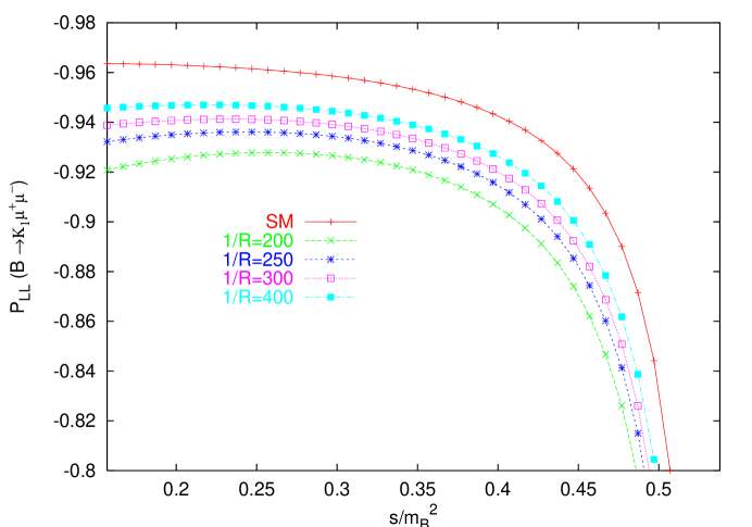
In Fig.1, we present the dependence of the PL​Lsubscript𝑃𝐿𝐿P_{LL} for the Bβ†’K1​μ+β€‹ΞΌβˆ’β†’π΅subscript𝐾1superscriptπœ‡superscriptπœ‡B\rightarrow K_{1}\mu^{+}\mu^{-} decay as a function of s/mB2𝑠superscriptsubscriptπ‘šπ΅2s/m_{B}^{2}. We see that, PL​Lsubscript𝑃𝐿𝐿P_{LL} in UED compatible with the SM result. Increasing s^^𝑠\hat{s}, PL​Lsubscript𝑃𝐿𝐿P_{LL} is moderate for the low of s^^𝑠\hat{s}. The effect of KK contribution in the Wilson coefficient are consistent for 1/R=200​G​e​V1𝑅200𝐺𝑒𝑉1/R=200GeV at low value of s^^𝑠\hat{s}. 1/R=200​G​e​V1𝑅200𝐺𝑒𝑉1/R=200GeV value is greater than 1/R=400​G​e​V1𝑅400𝐺𝑒𝑉1/R=400GeV. 
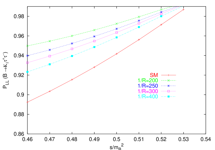
In Fig.2, Double lepton longitudinal polarization asymmetries for the Bβ†’K1​τ+β€‹Ο„βˆ’β†’π΅subscript𝐾1superscript𝜏superscript𝜏B\rightarrow K_{1}\tau^{+}\tau^{-} decay is presented, From this figure is follows, UED model prediction coincide with the SM result. One can see that the value of the longitudinal polarization is different in the low of s^^𝑠\hat{s} for the Bβ†’K1​τ+β€‹Ο„βˆ’β†’π΅subscript𝐾1superscript𝜏superscript𝜏B\rightarrow K_{1}\tau^{+}\tau^{-} decay. While 1/R=200​G​e​V1𝑅200𝐺𝑒𝑉1/R=200GeV value is max in the UED model, The SM result is approximately two times lower than this value.
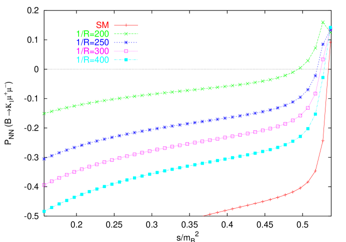
 In Fig.3, For the Bβ†’K1​μ+β€‹ΞΌβˆ’β†’π΅subscript𝐾1superscriptπœ‡superscriptπœ‡B\rightarrow K_{1}\mu^{+}\mu^{-} decay, we analysis to the normal polarizations. We obtained good result at the 1/R=200​G​e​V1𝑅200𝐺𝑒𝑉1/R=200GeV in UED model. We can see that the effect of extra dimension are very noticeable at the small value of s^^𝑠\hat{s}. When the value of s^^𝑠\hat{s} close to 0.20.20.2, all the value of normal polarization is coincide with each other. In s^=0.36^𝑠0.36\hat{s}=0.36, the value of 1/R=200​G​e​V1𝑅200𝐺𝑒𝑉1/R=200GeV is five times bigger than SM result. 
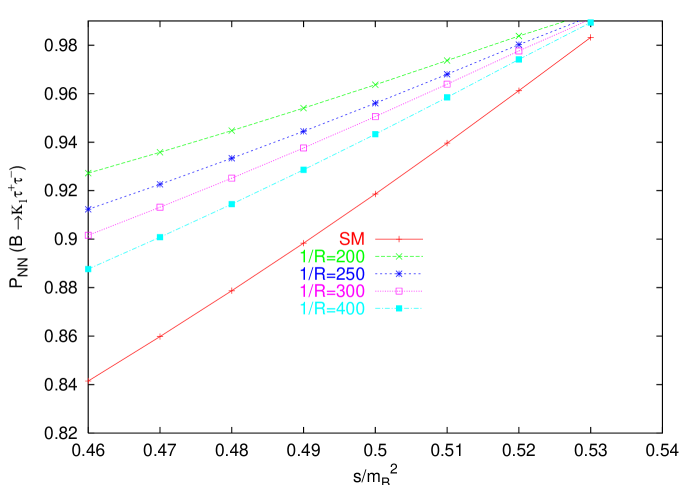
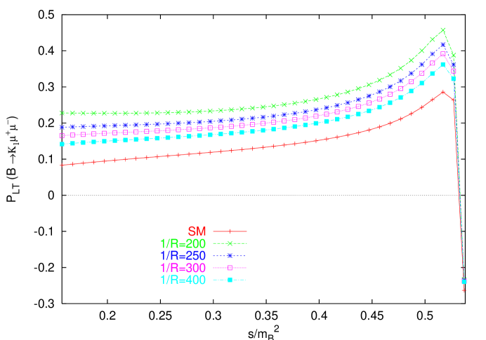
But in Fig.4, for the Bβ†’K1​τ+β€‹Ο„βˆ’β†’π΅subscript𝐾1superscript𝜏superscript𝜏B\rightarrow K_{1}\tau^{+}\tau^{-} decay, it is similar to the PL​Lsubscript𝑃𝐿𝐿P_{LL} result. 
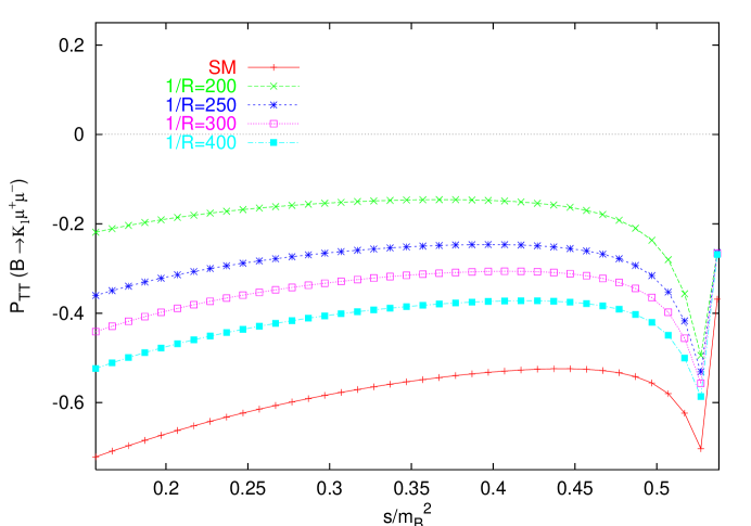
In Fig.5, We examine to the transversal polarization for the Bβ†’K1​μ+β€‹ΞΌβˆ’β†’π΅subscript𝐾1superscriptπœ‡superscriptπœ‡B\rightarrow K_{1}\mu^{+}\mu^{-} decay. At the 1/R=200​G​e​V1𝑅200𝐺𝑒𝑉1/R=200GeV value, we compared to that of the SM prediction PT​Tsubscript𝑃𝑇𝑇P_{TT} is larger from SM. Again, the effects of extra dimension are distinguished at the small value of momentum transfer s^^𝑠\hat{s} where PT​Tsubscript𝑃𝑇𝑇P_{TT} is minimum. For the s^=0.53^𝑠0.53\hat{s}=0.53 value, all polarization values are decreases. 
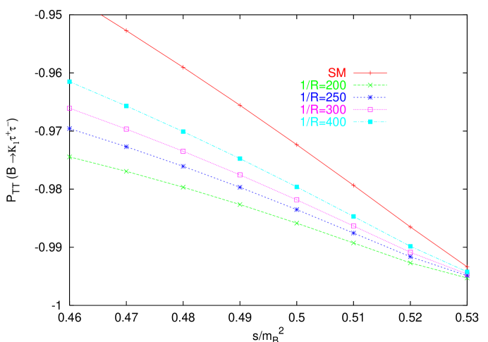
In Fig.6, We analysis to transversal polarization as a function of the s^^𝑠\hat{s} for the Bβ†’K1​τ+β€‹Ο„βˆ’β†’π΅subscript𝐾1superscript𝜏superscript𝜏B\rightarrow K_{1}\tau^{+}\tau^{-} decay. We observe a little contributions from UED model, especially in the 1/R=400​G​e​V1𝑅400𝐺𝑒𝑉1/R=400GeV value. But UED model is better than SM in this figure. All model values come together with the SM result in the s^=0.53^𝑠0.53\hat{s}=0.53 
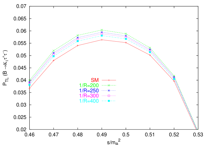
value. In Fig.7, we investigate PL​Tsubscript𝑃𝐿𝑇P_{LT} polarization. We see that increasing s^^𝑠\hat{s}, PL​Tsubscript𝑃𝐿𝑇P_{LT} increase until s^=0.5​G​e​V2^𝑠0.5𝐺𝑒superscript𝑉2\hat{s}=0.5GeV^{2}. After this value of s^^𝑠\hat{s} two models are decrease until s^=0.55​G​e​V2^𝑠0.55𝐺𝑒superscript𝑉2\hat{s}=0.55GeV^{2}. (PL​T)U​E​D=2​(PL​T)S​Msubscriptsubscriptπ‘ƒπΏπ‘‡π‘ˆπΈπ·2subscriptsubscript𝑃𝐿𝑇𝑆𝑀(P_{LT})_{UED}=2(P_{LT})_{SM} at 1/R=200​G​e​V1𝑅200𝐺𝑒𝑉1/R=200GeV. So It is also very useful for establishing new physics. In Fig.8, We show our predictions for the PT​Lsubscript𝑃𝑇𝐿P_{TL} for Bβ†’K1​τ+β€‹Ο„βˆ’β†’π΅subscript𝐾1superscript𝜏superscript𝜏B\rightarrow K_{1}\tau^{+}\tau^{-} decay. We get |(PT​L)U​E​D|>|(PT​L)S​M|subscriptsubscriptπ‘ƒπ‘‡πΏπ‘ˆπΈπ·subscriptsubscript𝑃𝑇𝐿𝑆𝑀|(P_{TL})_{UED}|>|(P_{TL})_{SM}|. This result can serve as a good test for discrimination of two models. The other polarizations for the Bβ†’K1​l+​lβˆ’β†’π΅subscript𝐾1superscript𝑙superscript𝑙B\rightarrow K_{1}l^{+}l^{-} decay, we have imaginary part and therefore there is no interference terms between SM and UED model contributions.

In conclusion, we have studied the double-lepton polarization asymmetries in the UED model. We obtain different double-lepton polarization asymmetries which is very sensitive to the UED model. It has been shown that all these physical observebles are very sensitive to the existence of new physics beyond SM and their experimental measurements can give valuable information on it.

Acknowledgements

The author would like to thank T. M. Aliev, M. SavcΔ± and A. Ozpineci for useful discussions during the course of the work.

Refer to caption
Figure 1: The dependence of the Longitudinal polarization,for $B\rightarrow K_{1}\mu^{+}\mu^{-}$ decay, as a function of the $\hat{s}$ .
Refer to caption
Figure 2: The dependence of the Longitudinal polarization,for $B\rightarrow K_{1}\tau^{+}\tau^{-}$ decay, as a function of the $\hat{s}$ . .
Refer to caption
Figure 3: The dependence of the Normal polarization,for $B\rightarrow K_{1}\mu^{+}\mu^{-}$ decay, as a function of the $\hat{s}$ .
Refer to caption
Figure 4: The dependence of the Normal polarization,for $B\rightarrow K_{1}\tau^{+}\tau^{-}$ decay, as a function of the $\hat{s}$ .
Refer to caption
Figure 5: The dependence of the Transversal polarization,for $B\rightarrow K_{1}\mu^{+}\mu^{-}$ decay, as a function of the $\hat{s}$ .
Refer to caption
Figure 6: The dependence of the Transversal polarization,for $B\rightarrow K_{1}\tau^{+}\tau^{-}$ decay, as a function of the $\hat{s}$ .
Refer to caption
Figure 7: The dependence of the $P_{LT}$ polarization,for $B\rightarrow K_{1}\mu^{+}\mu^{-}$ decay, as a function of the $\hat{s}$ .
Refer to caption
Figure 8: The dependence of the $P_{TL}$ polarization,for $B\rightarrow K_{1}\tau^{+}\tau^{-}$ decay, as a function of the $\hat{s}$ .

References

  • [1] K. Abe, et al.,Belle Collaboration Prep, hep-ex/0410006, (2004) .
  • [2] B. Aubert, et al.,BaBar Collaboration Phys. Rev. Lett. 93, 081802, (2004) .
  • [3] T. Mannel and S. Recksiegel, J. Phys., G 24 (1998) 979.
  • [4] A. Ali, P. Ball, L. T. Handoko and G. Hiller, Phys. Rev., D 61 (2000) 074024 [arXiv : hep-ph/9910221].
  • [5] T. M. Aliev, M. K. Cakmak and M.Savci, Nucl. Phys. ,B 607 (2001) 305 [arXiv : hep-ph/0009133]; T. M. Aliev, A. Ozpineci, M. Savci and C. Yuce, Phys. Rev. ,D 66 (2002) 115006 [arXiv : hep-ph/0208128].
  • [6] F.Kruger and E. Lunghi, Phys. Rev. ,D 63 (2001) 014013 [arXiv : hep-ph/0008210].
  • [7] S. Rai Choudhury, N. Gaur and N. Mahojan Phys. Rev.,D 66, (2002) 054003.
  • [8] U. O. Yilmaz, B. B. Sirvanli and G. Turan, Nucl. Phys.,B 692 (2004) 249 [arXiv : hep-ph/0407006].
  • [9] W. Bensalem, D. London, N. Sinha and R. Sinha, Phys. Rev. ,D 67 (2003) 034007.
  • [10] T. Appelquist, H. C. Cheng and B. A. Dobrescu, Phys. Rev ,D 64 (2001) 035002.
  • [11] A. J. Buras, M. Sprander and A. Weiler, Nucl. Phys. ,B 660 (2003) 225.
  • [12] A. J. Buras, A. Poschenrieder, M. Sprander and A. Weiler, Nucl. Phys. ,B 678 (2004) 455.
  • [13] T. M. Aliev, M. Savci and B. B. Sirvanli, Eur. Phys. J.,C 52,(2007) 375-382 [arXiv : hep-ph/0608143].
  • [14] I. Ahmed, M. A. Paracha and M. J. Aslam Eur. Phys. J.,C 54,(2008) 591-599 [arXiv : hep-ph/08020740].
  • [15] A. J. Buras et al. Nucl. Phys.,B 424 (1994) 374.
  • [16] P. Colangelo, F. De Fazio, R. Ferrendes, T. N. Pham, Prep : hep-ph/ 0604029,(2006).
  • [17] M. A. Paracha, I. Ahmed, M. J. Aslam, Eur. Phys. J. ,C 52 (2007) 967-973 [arXiv : hep-ph/07070733].
  • [18] A. H. S. Gilani, Riazuddin and T. A. Al-Aithan, JHEP,09 (2003) 065.
  • [19] C. A. Dominguez, N. Paver and Riazuddin, Phys. Lett. ,B 214 (1988) 459.
  • [20] A. Saddique, M. J. Aslam and C.D. L , [arXiv : hep-ph/08030192].