IFJPAN-IV-2008-6

Markovian MC simulation of QCD evolution at NLO level with minimum $k_{T}$ ^⋆

P. Stokłosa^a, W. Płaczek^b, and M. Skrzypek^a

^aInstitute of Nuclear Physics IFJ-PAN,
ul. Radzikowskiego 152, 31-342 Cracow, Poland.
^bMarian Smoluchowski Institute of Physics, Jagiellonian University,
ul. Reymonta 4, 30-059 Cracow, Poland.

We present two Monte Carlo algorithms of the Markovian type which solve the modified QCD evolution equations at the NLO level. The modifications with respect to the standard DGLAP evolution concern the argument of the strong coupling constant $\alpha_{S}$. We analyze the $z$-dependent argument and then the $k_{T}$-dependent one. The evolution time variable is identified with the rapidity. The two algorithms are tested to the $0.05$% precision level. We find that the NLO corrections in the evolution of parton momentum distributions with $k_{T}$-dependent coupling constant are of the order of 10 to 20%, and in a small $x$ region even up to 30%, with respect to the LO contributions.

IFJPAN-IV-2008-6

^⋆The project is partly supported by the EU grant MTKD-CT-2004-510126, realized in the partnership with the CERN Physics Department and by the Polish Ministry of Science and Information Society Technologies grant No 620/E-77/6.PR UE/DIE 188/2005-2008.

1 Introduction

With the first LHC results coming soon the precision of the QCD calculations becomes an important issue. As usuall, one finds two approaches to the calculations: fixed-order calculations and resumed to all orders Monte Carlo (MC) parton showers. The fixed-order results are impressive. Let us give a few examples of such calculations: the splitting functions, calculated up to NNLO level [1, 2] or various differential and semi-inclusive distributions, calculated in the NNLO and even NNNLO approximation see e.g. [3, 4, 5]. On the other hand, the MC parton shower approach, indispensable in describing complicated experimental signal selection procedures, does not achieve such a high precision. In fact, the complete NLO level has not been reached yet by any of the available MC parton shower codes. In most of the cases these codes are based on some form of an improved LO approximation, see e.g. [6, 7, 8, 9, 10]. Another approach is based on combining the NLO matrix element with the LO parton shower [11, 12].

Some time ago some of us started the MC parton shower project with the ambitious goal of reaching the NLO precision level. The project is based on the DGLAP evolution equation [13] at the NLO level [14, 15, 16, 17]. We began by creating two different algorithms, and then constructing two MC programs, that solve the evolution equation and simulate the one-hemisphere collinear parton shower. First algorithm, called EvolFMC (Markovian Monte Carlo), is based on the principle of a Markovian process. It generates the DGLAP-type evolution of Parton Distribution Functions (PDFs) up to the NLO level including both gluons and quarks. In Ref. [18] we have shown for the first time that with the aid of modern CPU such a MC code can solve the LO evolution equations with the precision below $10^{-3}$, i.e. comparable or even better than the other numerical methods. This study has been extended to the NLO evolution in Ref. [19]. The second algorithm called CMC is an entirely new type of an algorithm, an example of a wider class that we named ”Constrained Markovian Monte Carlo”. CMC is designed to solve the Markovian evolution with superimposed constraint on both $x$ and flavor type of the outgoing parton [20, 21]. Such an evolution with predefined end-point, mandatory for the simulation of the resonant processes, is an alternative for the commonly used workaround solution of this problem based on the so-called ”backward evolution” [22]. The ultimate goal is to combine two initial-state non-collinear NLO constrained evolutions (in two hemispheres) together with the hard process into one NLO parton shower for the Drell-Yan-type processes, either in full agreement with the DGLAP evolution or including effects of a modified-DGLAP type.

The EvolFMC code includes also the modified DGLAP evolutions in which the argument of the coupling constant is replaced by more complicated functions of $x$, $x^{\prime}$ and $Q^{2}$ [23, 24, 25, 26, 27]. In particular, the use of $k_{T}$ as the argument is known to effectively resum some of the higher order soft corrections [23, 26, 28]. For this reason it is the preferred choice of most of the MC parton shower codes. The $k_{T}$ is used as an argument also by the CCFM evolution equation [29]. This equation is designed to effectively interpolate between the DGLAP evolution in the large $x$ region and the BFKL-type behavior in the low $x$ region. The CCFM equation uses, apart from the modified arguments of coupling constant and angular ordering, also the ”non-Sudakov form factor”, important in the small $x$ region.

In the case of the developed by us EvolFMC code the option of modified argument of the coupling constant has been so far implemented only in the LO approximation [30, 31]. This is a significant limitation since both the NLO kernels and the $k_{T}$-dependent coupling constant are important for the final precision of the parton shower. In the present paper we will fill in this gap and present the NLO extension of the $k_{T}$-dependent EvolFMC code. In this scheme the evolution variable is understood to be the rapidity of emitted partons, ensuring the angular ordering. We will discuss also another choice of the argument: $Q(1-z)$. It is based on the variant of the CCFM equation, called the ”one-loop” CCFM [32, 33]. Of course, $Q(1-z)$ is only one of a few $z$-dependent functions that have been used in the literature [24, 25, 34].

The primary role of the presented here Markovian NLO code would be to serve as a powerfull testing device capable of reproducing independently any of the above evolution types. In particular, the emulation of the CCFM equation would be possible, if the collinear evolution is supplied with the transverse momenta and the ”non-Sudakov form factor” is added. Another area of application of such a Markovian MC would be in performing fits of the PDFs to the $F_{2}$ data. We have demonstrated recently [35] that using MC codes for the purpose of fitting is feasible with the modern computer power. Finally, for the simulation of the final-state parton shower, the Markovian algorithm without constraints is directly applicable.

Let us digress here that the standard evolution kernels of the collinear factorisation, either LO or NLO, are used in the normal integrated form, i.e. as functions of the $x$ and $t$ variables only. This is of course the well-established and extremely successful DGLAP approach. Nonetheless, for more exclusive observables at the LHC, it will be necessary to include the effects of transverse momenta beyond the collinear approximation. Some attempts in this direction have already been made, for example by the above mentioned MC$@$NLO [11, 12], the GR$@$PPA project [36, 37] or the CCFM-based [29] CASCADE project [38].

Another interesting approach is based on the idea of ”exclusive” DGLAP kernels in which the internal degrees of freedom are not integrated out analytically, but instead simulated (i.e. integrated) by the MC parton shower itself [39].

Finally, let us comment on yet another class of MC algorithms solving the evolution equations – the veto algorithms [40, 41, 42]. They are based on a Markovian evolution with additional internal pseudo-emission loop. Thanks to this feature it is enough to compute an approximate Sudakov form factor, instead of the exact one, for each of the generated events and the algorithm becomes faster. On the negative side, the average multiplicity of the generated partons is much higher. We did not use the veto scheme in this work. The main reason for this is that, as discussed earlier, we consider Markovian-type algorithms primarily as a testing device for the constrained Markovian algorithms. In these latter cases the veto algorithm does not apply and the Sudakov form factors must be calculated. For that reason we preferred to have the Sudakov form factors implemented (and mutually tested) in both approaches.

This paper is organized as follows. In the next Section we introduce all necessary notation, briefly present the general formalism of the Markovian MC solutions of the evolution equations and define two particular evolution schemes that we are interested in. In the following two Sections we describe in detail the MC algorithms that solve the above two evolutions by means of the collinear Markovian parton shower. We present two algorithms, main and auxiliary (mostly for tests), for each of the schemes. As the simpler ones we discuss in detail the $Q(1-z)$-type algorithms, whereas in the description of the $k_{T}$-dependent ones we focus mostly on the modifications with respect to the $Q(1-z)$-type algorithms. In Section 5 we present numerical results: first we discuss the choice of the counter term and input parameters, then we briefly describe a variety of technical tests that we performed in order to establish the technical precision of the EvolFMC code, and finally we compare and discuss various types of evolution. The Summary Section concludes the paper.

2 General framework

In this paper we will follow the general formulation of the evolution equation and its solutions in terms of the Markovian MC presented in Ref. [42]. In order to establish the notation let us recall here basic definitions and formulas. For more complete presentation we refer the reader to the Ref. [42]. We write the evolution equation in the compact matrix notation

$$\partial_{t}{\bf D}(t)={\bf K}(t)\;{\bf D}(t)$$ (1)

and in the explicit representation

$$\partial_{t}D_{f}(t,x)=\sum_{f^{\prime}}\int_{x}^{1}dw\;\mathcal{K}_{ff^{\prime}}(t,x,w)D_{f^{\prime}}(t,w),$$ (2)

where $D_{f}(t,w)$ denotes the parton density function of the parton $f$ and $\mathcal{K}_{ff^{\prime}}(t,x,w)$ denotes the generalized evolution kernel. Note that contrary to the DGLAP case, it depends on two variables, $x$ and $w$, instead of their ratio $z=x/w$ only. The kernel is then decomposed into real and virtual parts

$$\begin{split}&\mathcal{K}_{ff^{\prime}}(t,x,w)=\mathcal{K}^{V}_{ff^{\prime}}(t,x,w)+\mathcal{K}^{R}_{ff^{\prime}}(t,x,w),\quad\mathcal{K}^{V}_{ff^{\prime}}(t,x,w)=-\delta_{ff^{\prime}}\delta_{x=w}\mathcal{K}^{v}_{ff}(t,x).\end{split}$$ (3)

The Markovian solution of eq. (1) is conveniently expressed with the help of the operator $\bar{\bf E}$ defined as

$$\bar{\bf E}\;{\bf D}(t)\equiv\int_{0}^{1}dx\sum_{f}x\;D_{f}(t,x),\quad\hbox{i.e.}\quad\bar{E}_{f}(x)\equiv x.$$ (4)

This operator in a formal way shows that we use an ”unconstrained” evolution – all values of $x$ and $f$ will be generated and that the evolution will be done for momentum distributions $x\bf D(t)$. The solution of eq. (1) and the master formula for the Markovian MC is then

$$\begin{split}\bar{\bf E}{\bf D}(t)=\int_{t_{0}}^{t}dt_{1}\bigg{(}\int_{t_{1}}^{t}dt_{2}\bigg{[}&\int_{t_{2}}^{t}dt_{3}\bigg{\{}\dots\\ \dots\int_{t_{N-1}}^{t}dt_{N}\bigg{\{}&\bar{\bf E}{\bf K}^{R}(t_{N}){\bf G}_{{\bf K}^{V}}(t_{N},t_{N-1})+\bar{\bf E}{\bf G}_{{\bf K}^{V}}(t,t_{N-1})\delta_{t_{N}=t}\bigg{\}}\\ ~{}~{}~{}~{}~{}~{}~{}~{}~{}~{}~{}~{}~{}\vdots\\ \times&{\bf K}^{R}(t_{2}){\bf G}_{{\bf K}^{V}}(t_{2},t_{1})+\bar{\bf E}{\bf G}_{{\bf K}^{V}}(t,t_{1})\delta_{t_{2}=t}\bigg{]}\\ \times&{\bf K}^{R}(t_{1}){\bf G}_{{\bf K}^{V}}(t_{1},t_{0})+\bar{\bf E}{\bf G}_{{\bf K}^{V}}(t,t_{0})\delta_{t_{1}=t}\bigg{)}{\bf D}(t_{0}),\end{split}$$ (5)

where the diagonal matrix ${\bf G}_{{\bf K}^{V}}$ is the solution of the evolution equation with the virtual kernel $\mathcal{K}^{V}_{ff^{\prime}}(t,x,w)$ parametrized in terms of the Sudakov form factor $\Phi_{f}(t,t^{\prime}|x)$:

$$\{{\bf G}_{{\bf K}^{V}}(t,t^{\prime})\}_{ff^{\prime}}(x,w)=\delta_{ff^{\prime}}\delta_{x=w}\;e^{-\Phi_{f}(t,t^{\prime}|w)},\qquad\Phi_{f}(t,t^{\prime}|x)=\int_{t^{\prime}}^{t}dt^{\prime\prime}\;\mathcal{K}^{v}_{ff}(t^{\prime\prime},x).$$ (6)

The above formula (5) follows from the iteration of the momentum conservation principle

$$\int\limits_{t_{i-1}}^{t}dt_{i}\;\Big{\{}\bar{\bf E}{\bf K}^{R}(t_{i}){\bf G}_{{\bf K}^{V}}(t_{i},t_{i-1})+\bar{\bf E}{\bf G}_{{\bf K}^{V}}(t,t_{i-1})\delta_{t_{i}=t}\Big{\}}=\bar{\bf E}.$$ (7)

Eq. (7) defines also the probabilities of the single step forward in $t_{i},f_{i}$ and $x_{i}$ variables:

$$\begin{split}1&=\frac{1}{x_{i-1}}\int\limits_{t_{i-1}}^{t}dt_{i}\;\Big{\{}\bar{\bf E}{\bf K}^{R}(t_{i}){\bf G}_{{\bf K}^{V}}(t_{i},t_{i-1})+\bar{\bf E}{\bf G}_{{\bf K}^{V}}(t,t_{i-1})\delta_{t_{i}=t}\Big{\}}_{f_{i-1}}(x_{i-1})\\ &=e^{-\Phi_{f_{i-1}}(t,t_{i-1}|x_{i-1})}+\int\limits^{1}_{e^{-\Phi_{f_{i-1}}(t,t_{i-1}|x_{i-1})}}d\left(e^{-\Phi_{f_{i-1}}(t_{i},t_{i-1}|x_{i-1})}\right)\\ &~{}~{}~{}~{}\times\left[\sum_{f_{i}}\frac{\partial_{t_{i}}\Phi_{f_{i}f_{i-1}}(t_{i},t_{i-1}|x_{i-1})}{\partial_{t_{i}}\Phi_{f_{i-1}}(t_{i},t_{i-1}|x_{i-1})}\int dx_{i}\;\frac{1}{\partial_{t_{i}}\Phi_{f_{i}f_{i-1}}(t_{i},t_{i-1}|x_{i-1})}\frac{x_{i}}{x_{i-1}}\mathcal{K}^{R}_{f_{i}f_{i-1}}(t_{i},x_{i},x_{i-1})\right],\end{split}$$ (8)

where the virtual Sudakov form factor is expressed in terms of the real emission part of the evolution kernel

$$\begin{split}\Phi_{f_{i-1}}(t_{i},t_{i-1}|x_{i-1})=&\int\limits^{t_{i}}_{t_{i-1}}dt\;{\mathcal{K}^{v}_{f_{i-1}f_{i-1}}(t,x_{i-1})}\\ =&\sum_{f_{i}}\int\limits^{t_{i}}_{t_{i-1}}dt\int\limits_{0}^{x_{i-1}}\frac{dx_{i}}{x_{i-1}}x_{i}\;\mathcal{K}^{R}_{f_{i}f_{i-1}}(t,x_{i},x_{i-1})=\sum_{f_{i}}\Phi_{f_{i}f_{i-1}}(t_{i},t_{i-1}|x_{i-1}).\end{split}$$ (9)

In the case of a weighted algorithm with the global correcting weight, one uses the simplified kernel $\mathcal{K}^{R}_{f_{i}f_{i-1}}(t_{i},x_{i},x_{i-1})\to\bar{\mathcal{K}}^{R}_{f_{i}f_{i-1}}(t_{i},x_{i},x_{i-1})$. This simplification is compensated by the global weight

$$w^{(n)}=e^{\bar{\Phi}_{f_{n}}(t,t_{n}|x_{n})-\Phi_{f_{n}}(t,t_{n}|x_{n})}\left(\prod_{i=1}^{n}\frac{\mathcal{K}^{R}_{f_{i}f_{i-1}}(t_{i},x_{i},x_{i-1})}{\bar{\mathcal{K}}^{R}_{f_{i}f_{i-1}}(t_{i},x_{i},x_{i-1})}e^{\bar{\Phi}_{f_{i-1}}(t_{i},t_{i-1}|x_{i-1})-\Phi_{f_{i-1}}(t_{i},t_{i-1}|x_{i-1})}\right),$$ (10)

where $n$ denotes the number of emissions generated within a given MC event, and the form factor $\bar{\Phi}_{f_{i-1}}(t_{i},t_{i-1}|x_{i-1})$ is constructed from $\bar{\mathcal{K}}^{R}_{f_{i}f_{i-1}}(t_{i},x_{i},x_{i-1})$ in complete analogy to eq. (9). The last quantity to be defined here is the exact shape of the kernels, including the definition of the argument of the coupling constant in terms of the $t$ and $x$ variables. Following Ref. [42] we will discuss two schemes of modified-DGLAP type, denoted in Ref. [42] as (B’) and (C’). The novelty with respect to Ref. [42] is that we will perform the calculation and construct the Markovian MC code at the NLO level, whereas in Ref. [42] only the LO case has been discussed. To be specific, the schemes are defined as

$$\begin{split}&x\mathcal{K}^{R(B^{\prime})}_{f^{\prime}f}(t,x,w)=\\ &=\biggl{(}\frac{\alpha_{NLO}(\ln(1-z)+t)}{2\pi}2zP_{f^{\prime}f}^{R(0)}(z)+\Bigl{(}\frac{\alpha_{NLO}(\ln(1-z)+t)}{2\pi}\Bigr{)}^{2}2zP_{f^{\prime}f}^{R(1)B^{\prime}}(z)\biggr{)}\theta_{1-z>\lambda e^{-t}},\\ &x\mathcal{K}^{R(C^{\prime})}_{f^{\prime}f}(t,x,w)=\\ &=\biggl{(}\frac{\alpha_{NLO}(\ln(w-x)+t)}{2\pi}2zP_{f^{\prime}f}^{R(0)}(z)+\Bigl{(}\frac{\alpha_{NLO}(\ln(w-x)+t)}{2\pi}\Bigr{)}^{2}2zP_{f^{\prime}f}^{R(1)C^{\prime}}(z)\biggr{)}\theta_{w-x>\lambda e^{-t}},\end{split}$$ (11)

where $z=x/w$ and $\lambda$ is the cut-off on the argument of the coupling constant. Note that $\lambda$ is not an infinitesimal IR cut-off, as used in the DGLAP case. On the contrary, $\lambda$ is finite, typically of the order of a few GeV. Note also that the factor 2 in front of the kernels is due to our definition of the evolution time, which in the DGLAP case is chosen as $t=\ln Q$ rather than $t=\ln Q^{2}$.

The NLO parts of the kernels, $P_{f^{\prime}f}^{R(1)B^{\prime}}(z)$ and $P_{f^{\prime}f}^{R(1)C^{\prime}}(z)$, consist of the universal part $P_{f^{\prime}f}^{R(1)}(z)$ [16, 17] and the evolution scheme dependent counter terms $\Delta P_{f^{\prime}f}^{R(1)B^{\prime}}(z)$ and $\Delta P_{f^{\prime}f}^{R(1)C^{\prime}}(z)$

$$\begin{split}P_{f^{\prime}f}^{R(1)B^{\prime}}(z)=&P_{f^{\prime}f}^{R(1)}(z)+\Delta P_{f^{\prime}f}^{R(1)B^{\prime}}(z),\\ P_{f^{\prime}f}^{R(1)C^{\prime}}(z)=&P_{f^{\prime}f}^{R(1)}(z)+\Delta P_{f^{\prime}f}^{R(1)C^{\prime}}(z).\end{split}$$ (12)

These counter terms are necessary to remove the double counting introduced by the shift of the arguments of the coupling constants. There is some freedom in defining these counter terms. The algorithms presented here work for any (reasonable) choice of the counter terms. For further details on the choice we used in this work we refer the reader to Section 5.1.

We will frequently be using also the representation of the universal parts of the kernels based on their structure in the $z$-variable

$$zP_{f^{\prime}f}^{R(0)}(z)= \,\frac{1}{1-z}\delta_{f^{\prime}f}A_{ff}^{(0)}+F_{f^{\prime}f}^{(0)}(z),$$

$$zP_{f^{\prime}f}^{R(1)}(z)= \,\frac{1}{1-z}\delta_{f^{\prime}f}A_{ff}^{(1)}(z)+F_{f^{\prime}f}^{(1)}(z).$$ (13)

The functions $P_{f^{\prime}f}^{R}(z)$, $A_{ff}(z)$ and $F_{f^{\prime}f}(z)$, written in the notation used here, are collected in Ref. [19].

The coupling constant at the NLO level has the standard form

$$\alpha_{LO}(t) =\frac{2\pi}{\beta_{0}(t-\ln\Lambda_{0})},$$

$$\alpha_{NLO}(t) =\alpha_{LO}(t)\left(1-\alpha_{LO}(t)\ \frac{\beta_{1}\ln(2t-2\ln\Lambda_{0})}{4\pi\beta_{0}}\right).$$ (14)

We close this general introduction with a brief explanation why we state that the argument $\ln(x_{i-1}-x_{i})+t_{i}$ can be regarded as $k^{T}_{i}$ of the emitted real parton with the four momentum $k_{i}$. It follows immediately from the kinematical mapping of the evolution variables into four momenta, provided that the evolution time is identified with the rapidity of the emitted parton and the $x$-variable, as usual, with the light-cone plus component of the virtual parton

$$t_{i}=\ln(2E_{h})-\frac{1}{2}\ln\frac{k_{i}^{+}}{k_{i}^{-}},\;\;\;k_{i}^{+}=2E_{h}(x_{i-1}-x_{i})$$ (15)

where $E_{h}$ is an arbitrary reference energy of the incoming hadron. As a consequence of the maslessness of $k_{i}$ we obtain

$$k^{T}_{i}=\sqrt{k^{+}k^{-}}=e^{t_{i}}(x_{i-1}-x_{i}).$$ (16)

Let us now proceed with the description of the novel NLO algorithms for the two schemes.

3 Markovian algorithm for scheme (B’)

In this section we will present two schemes of solving the evolution B’ in a Markovian way at the NLO level. We begin with the efficient one and then we present the other scheme, devised mostly for the testing purposes.

3.1 Main algorithm

The main algorithm is based on the simplified LO DGLAP kernel in which the coupling constant is used in the NLO approximation. Specifically we follow the eq. (3.21) of Ref. [30], see also [43], and we extend it to the NLO case

$$x\bar{\mathcal{K}}^{R(B^{\prime})}_{f^{\prime}f}(t,x,w)\equiv \frac{\alpha_{NLO}(t+\ln(1-z))}{2\pi}2z\bar{P}^{R(B^{\prime})}_{f^{\prime}f}(z)\theta_{1-z>\lambda e^{-t}},$$ (17)

$$z\bar{P}^{R(B^{\prime})}_{f^{\prime}f}(z)= \frac{1}{1-z}(\delta_{f^{\prime}f}A_{ff}^{(0)}+\max_{z}F^{(0)}_{f^{\prime}f}(z)+M_{f^{\prime}f}).$$ (18)

We remind the reader that $z=x/w$. Note that the singular factor $1/(1-z)$ is artificially introduced into the $F$-part in order to achieve analytical integrability of the formula, see Ref. [30] for more discussion. The constant $M_{f^{\prime}f}$ is defined as

$$M_{f^{\prime}f}=\left\{\begin{array}[]{c}0,\;\;\;\;{\rm if\;}P^{R(0)}_{f^{\prime}f}(z)\neq 0,\\ \eta,\;\;\;\;{\rm if\;}P^{R(0)}_{f^{\prime}f}(z)=0,\end{array}\right.$$ (21)

where $\eta$ is a dummy technical parameter. The reason behind introduction of $M_{f^{\prime}f}$ is very simple – we want to remove all zeroes in the LO transition matrix, because some of them might become non-zero at the NLO level and cause infinite weights. The constant $\eta$ is therefore added to all kernels that are zero at the LO level. Of course this is purely technical, dummy, operation, later on corrected by means of a proper rejection weight.

The corresponding Sudakov form factor, necessary to generate the time $t_{i}$, is then defined as

$$\bar{\Phi}_{f}^{B^{\prime}}(t_{i},t_{i-1}|x_{i-1})= \int_{t_{i-1}}^{t_{i}}dt\int_{0}^{1}d\Bigl{(}\frac{x}{w}\Bigr{)}\sum_{f^{\prime}}x\bar{\mathcal{K}}^{R(B^{\prime})}_{f^{\prime}f}(t,x,w)$$

$$= \frac{1}{\pi}\int_{t_{i-1}}^{t_{i}}dt\int^{t-t_{\lambda}}_{0}du\,\alpha_{NLO}(t-u)(A_{ff}^{(0)}+\sum_{f^{\prime}}(\max_{z}F^{(0)}_{f^{\prime}f}(z)+M_{f^{\prime}f}))$$

$$= \int_{t_{i-1}}^{t_{i}}dt\Bigl{(}\rho(t,t-t_{\lambda})-\rho(t,0)\Bigr{)}\Bigl{(}A_{ff}^{(0)}+\sum_{f^{\prime}}\max_{z}(F^{(0)}_{f^{\prime}f}(z)+M_{f^{\prime}f})\Bigr{)}$$

$$= (\bar{\zeta}(t_{i})-\bar{\zeta}(t_{i-1}))(A_{ff}^{(0)}+\sum_{f^{\prime}}(\max_{z}F^{(0)}_{f^{\prime}f}(z)+M_{f^{\prime}f})),$$ (22)

where

$$\rho(t,u) =\frac{1}{\pi}\int du\,\alpha_{NLO}(t-u)$$

$$=\frac{1}{\pi}\int{du}\frac{2}{\beta_{0}G(t,u)}\left(1-\frac{1}{2}\,{\frac{\beta_{1}\ln(2G(t,u))}{{\beta_{0}}^{2}G(t,u)}}\right)$$

$$=-\left(\frac{2}{\beta_{0}}+{\frac{\beta_{1}}{{\beta_{0}}^{3}G(t,u)}}\right)\ln(2G(t,u))-{\frac{\beta_{1}}{{\beta_{0}}^{3}G(t,u)}}$$

$$G(t,u) =t-u-\ln\Lambda_{0},\qquad u=-\ln(1-z),\qquad t_{\lambda}=\ln\lambda,$$ (23)

and

$$\bar{\zeta}(t) =a_{00}\left(\ln\left(t-\ln\Lambda_{0}\right)\right)^{2}+\left(a_{10}t+a_{11}\right)\ln\left(t-\ln\Lambda_{0}\right)+a_{20}t,$$ (24)

$$a_{00} =\frac{1}{2}\,{\frac{\beta_{1}}{{\beta_{0}}^{3}}},$$

$$a_{10} =\frac{2}{\beta_{0}},$$

$$a_{11} =-{\frac{2\,{\beta_{0}}^{2}\ln\Lambda_{0}-\beta_{1}\ln 2-\beta_{1}}{{\beta_{0}}^{3}}},$$

$$a_{20} =-\frac{\beta_{1}+2\beta_{0}^{2}(t_{\lambda}-\ln\Lambda_{0})}{\beta_{0}^{3}(t_{\lambda}-\ln\Lambda_{0})}\ln(t_{\lambda}-\ln\Lambda_{0})-\frac{2\beta_{0}^{2}(t_{\lambda}-\ln\Lambda_{0})+\beta_{1}(1+\ln 2)}{\beta_{0}^{3}(t_{\lambda}-\ln\Lambda_{0})}.$$

Let us note that the coefficients $a_{ij}$ need to be calculated only once during initialization of the algorithm. The procedure of inverting the function $\zeta(t_{i})$, necessary to generate the time $t_{i}$, has to be done numerically.

In the next step we generate the flavor index $f_{i}$ based on the probability

$$p_{f_{i}} =\frac{\partial_{t_{i}}\bar{\Phi}_{f_{i}f_{i-1}}^{B^{\prime}}(t_{i},t_{i-1}|x_{i-1})}{\partial_{t_{i}}\bar{\Phi}^{B^{\prime}}_{f_{i-1}}(t_{i},t_{i-1}|x_{i-1})}=\frac{\delta_{f_{i}f_{i-1}}A_{f_{i-1}f_{i-1}}^{(0)}+\max_{z}F^{(0)}_{f_{i}f_{i-1}}(z)+M_{f_{i}f_{i-1}}}{A_{f_{i-1}f_{i-1}}^{(0)}+\sum_{f_{i}}(\max_{z}F^{(0)}_{f_{i}f_{i-1}}(z)+M_{f_{i}f_{i-1}})},\;\;\;\sum_{f_{i}}p_{f_{i}}=1,$$ (25)

where

$${\partial_{t_{i}}\bar{\Phi}^{B^{\prime}}_{f_{i}f_{i-1}}(t_{i},t_{i-1}|x_{i-1})}= \int_{0}^{1}d\Bigl{(}\frac{x}{w}\Bigr{)}x\bar{\mathcal{K}}^{R(B^{\prime})}_{f_{i}f_{i-1}}(t_{i},x,w)$$

$$= \Bigl{(}\rho(t_{i},t_{i}-t_{\lambda})-\rho(t_{i},0)\Bigr{)}\Bigl{(}\delta_{f_{i}f_{i-1}}A_{f_{i-1}f_{i-1}}^{(0)}+\max_{z}F^{(0)}_{f_{i}f_{i-1}}(z)+M_{f_{i}f_{i-1}}\Bigr{)}$$ (26)

and

$${\partial_{t_{i}}\bar{\Phi}^{B^{\prime}}_{f_{i-1}}(t_{i},t_{i-1}|x_{i-1})}= \sum_{f_{i}}{\partial_{t_{i}}\bar{\Phi}^{B^{\prime}}_{f_{i}f_{i-1}}(t_{i},t_{i-1}|x_{i-1})}.$$ (27)

As the last variable we generate $z_{i}$. The normalized density distribution $dz_{i}p^{B^{\prime}}(z_{i})$ is given by

$$dz_{i}p^{B^{\prime}}(z_{i})= dz_{i}\frac{\alpha_{NLO}(t_{i}+\ln(1-z_{i}))}{\pi}\frac{\Theta_{1-z_{i}>\lambda e^{-t_{i}}}}{1-z_{i}}\biggl{(}\int_{0}^{1}dz\frac{\alpha_{NLO}(t_{i}+\ln(1-z))}{\pi}\frac{\Theta_{1-z>\lambda e^{-t_{i}}}}{1-z}\biggr{)}^{-1}$$

$$= du_{i}\frac{\alpha_{NLO}(t_{i}-u_{i})}{\pi}\Theta_{t_{i}-t_{\lambda}>u_{i}>0}\Bigl{(}\rho(t_{i},t_{i}-t_{\lambda})-\rho(t_{i},0)\Bigr{)}^{-1}$$

$$= du_{i}\partial_{u_{i}}\rho(t_{i},u_{i})\Theta_{t_{i}-t_{\lambda}>u_{i}>0}\Bigl{(}\rho(t_{i},t_{i}-t_{\lambda})-\rho(t_{i},0)\Bigr{)}^{-1}.$$ (28)

In the actual generation of $z_{i}$ we use the method of inverse cumulative. The $\rho(t_{i},u_{i})$ function has to be inverted numerically with respect to the $u_{i}$ variable.

The last part of the algorithm to be discussed here is the correcting weight, defined in eq. (10), compensating the simplification of the kernel done in eq. (17). The most complicated part of this weight is related to the exact Sudakov form factor. It has the form of the double integral. Numerical evaluation of such a double integral would significantly slow down the algorithm. Therefore it is essential to perform at least one of the integrations analytically. In the following we will show how this can be done in the NLO case.

Let us define the full Sudakov form factor $\Phi_{f}^{B^{\prime}}(t_{i},t_{i-1}|x_{i-1})$ of the B’ evolution

$$\Phi_{f}^{B^{\prime}}(t_{i},t_{i-1}|x_{i-1})= \int_{t_{i-1}}^{t_{i}}dt\int_{0}^{1}d\Bigl{(}\frac{x}{x_{i-1}}\Bigr{)}\sum_{f^{\prime}}x\mathcal{K}^{R(B^{\prime})}_{f^{\prime}f}(t,x,x_{i-1})$$

$$= \int_{t_{i-1}}^{t_{i}}dt\int_{0}^{1}dz\sum_{f^{\prime}}\biggl{(}\frac{\alpha_{S}(t+\ln(1-z))}{2\pi}2zP_{f^{\prime}f}^{R(0)}(z)$$

$$+\Bigl{(}\frac{\alpha_{S}(t+\ln(1-z))}{2\pi}\Bigr{)}^{2}2zP_{f^{\prime}f}^{R(1)B^{\prime}}(z)\biggr{)}\theta_{1-z>\lambda e^{-t}},$$ (29)

and let us write down the desired virtual component of the weight

$$\Delta_{f}^{B^{\prime}}(t_{i},t_{i-1}|x_{i-1})= \Phi_{f}^{B^{\prime}}(t_{i},t_{i-1}|x_{i-1})-\bar{\Phi}_{f}^{B^{\prime}}(t_{i},t_{i-1}|x_{i-1})$$

$$= \int_{t_{i}}^{t_{i-1}}dt\int_{0}^{1}dz\theta_{1-z>\lambda e^{-t}}\sum_{f^{\prime}}\biggl{(}\frac{\alpha_{S}(t+\ln(1-z))}{2\pi}2z\bigl{(}P_{f^{\prime}f}^{R(0)}(z)-\bar{P}_{f^{\prime}f}^{R(0)}(z)\bigr{)}$$

$$+\Bigl{(}\frac{\alpha_{S}(t+\ln(1-z))}{2\pi}\Bigr{)}^{2}2zP_{f^{\prime}f}^{R(1)B^{\prime}}(z)\biggr{)}.$$ (30)

The integral over $dz$ for general form of the kernel cannot be performed analytically even at the LO level (cf. Ref. [30]). However, as in the LO case of Ref. [30], the $dt$ integral can be done analytically also for the NLO case. The calculation looks as follows. We introduce the usual variable $u=-\ln(1-z)$ and then change order of integration. The resulting integral can be expressed as a sum of two integrals over the two regions of the $tu$ space shown in Fig. 1:

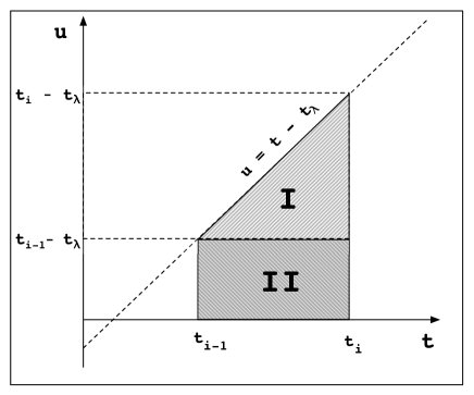
Figure 1: The integration domain in the $tu$ space for the case B’. Regions I and II correspond to two integrals in eq. (31).

$$\int_{t_{i-1}}^{t_{i}}dt\int_{0}^{1}dz\theta_{1-z>\lambda e^{-t}}= \int_{t_{i-1}}^{t_{i}}dt\int_{0}^{t-t_{\lambda}}du\,e^{-u}$$

$$= \int_{t_{i-1}-t_{\lambda}}^{t_{i}-t_{\lambda}}due^{-u}\int_{u+t_{\lambda}}^{t_{i}}dt+\int_{0}^{t_{i-1}-t_{\lambda}}due^{-u}\int_{t_{i-1}}^{t_{i}}dt.$$ (31)

The $dt$ integral, which depends on the coupling constant only, can be done analytically with the help of the integrals

$$\frac{1}{\pi}J_{1}(t,u)= \frac{1}{\pi}\int dt\alpha_{NLO}(t-u)=-\rho(t,u)$$ (32)

and

$$\frac{1}{\pi^{2}}J_{2}(t,u) =\frac{1}{\pi^{2}}\int dt\alpha_{NLO}^{2}(t-u)$$

$$=\int dt{\frac{\left(-2\,{\beta_{0}}^{2}(t-u-\ln\Lambda_{0})+\beta_{1}\ln 2\left(t-u-\ln\Lambda_{0}\right)\right)^{2}}{\beta_{0}^{6}\left(t-u-\ln\Lambda_{0}\right)^{4}}}$$

$$=\frac{a_{00}}{G^{3}(t,u)}\ln^{2}(2G(t,u))+\biggl{(}\frac{a_{10}}{G^{3}(t,u)}+\frac{a_{11}}{G^{2}(t,u)}\biggr{)}\ln(2G(t,u))$$

$$\;\;\;+\frac{a_{20}}{G^{3}(t,u)}+\frac{a_{30}}{G^{2}(t,u)}+\frac{a_{40}}{G(t,u)},$$ (33)

where

$$a_{00} =-\frac{1}{3}\frac{\beta_{1}^{2}}{\beta_{0}^{6}},\;\;\;a_{10}=-\frac{2}{9}\frac{\beta_{1}^{2}}{\beta_{0}^{6}},\;\;\;a_{11}=\frac{4\beta_{1}}{\beta_{0}^{4}},\;\;\;a_{20}=-\frac{2}{27}\frac{\beta_{1}^{2}}{\beta_{0}^{6}},\;\;\;a_{30}=\frac{\beta_{1}}{\beta_{0}^{4}},\;\;\;a_{40}=-\frac{4}{\beta_{0}^{2}}.$$

Collecting together the above results we can rewrite eq. (3.1) as

$$\Delta_{f}^{B^{\prime}} (t_{i},t_{i-1}|x_{i-1})=$$

$$= \int_{t_{i-1}-t_{\lambda}}^{t_{i}-t_{\lambda}}due^{-u}2z\sum_{f^{\prime}}\biggl{(}\frac{(J_{1}(t_{i},u)-J_{1}(u+t_{\lambda},u))}{2\pi}\bigl{(}P_{f^{\prime}f}^{R(0)}(z)-\bar{P}_{f^{\prime}f}^{R(B^{\prime})}(z)\bigr{)}$$

$$+\frac{(J_{2}(t_{i},u)-J_{2}(u+t_{\lambda},u))}{4\pi^{2}}P_{f^{\prime}f}^{R(1)B^{\prime}}(z)\biggr{)}$$

$$+\int_{0}^{t_{i-1}-t_{\lambda}}due^{-u}2z\sum_{f^{\prime}}\biggl{(}\frac{(J_{1}(t_{i},u)-J_{1}(t_{i-1},u))}{2\pi}\bigl{(}P_{f^{\prime}f}^{R(0)}(z)-\bar{P}_{f^{\prime}f}^{R(B^{\prime})}(z)\bigr{)}$$

$$+\frac{(J_{2}(t_{i},u)-J_{2}(t_{i-1},u))}{4\pi^{2}}P_{f^{\prime}f}^{R(1)B^{\prime}}(z)\biggr{)}$$ (34)

where $z=1-e^{-u}$. Note the cancellation of the leading singularity, $A_{ff}^{(0)}/(1-z)$, in the above formula due to

$$\sum_{f^{\prime}}z\Bigl{(}P_{f^{\prime}f}^{R(0)}(z)-\bar{P}_{f^{\prime}f}^{R(B^{\prime})}(z)\Bigr{)}=\sum_{f^{\prime}}\Biggl{(}F_{f^{\prime}f}^{(0)}(z)-\frac{1}{1-z}\biggl{(}\max_{z}F_{f^{\prime}f}^{(0)}(z)+M_{f^{\prime}f}\biggr{)}\Biggr{)}.$$ (35)

Combining together the real and virtual components we arrive at the final formula for the global weight of eq. (10) adopted to the case of the scheme B’

$$w^{(n)(B^{\prime})}=e^{-\Delta_{f_{n}}^{B^{\prime}}(t,t_{n}|x_{n})}\prod_{i=1}^{n}\left(\frac{\mathcal{K}^{R(B^{\prime})}_{f_{i}f_{i-1}}(t_{i},x_{i},x_{i-1})}{\bar{\mathcal{K}}^{R(B^{\prime})}_{f_{i}f_{i-1}}(t_{i},x_{i},x_{i-1})}e^{-\Delta_{f_{i-1}}^{B^{\prime}}(t_{i},t_{i-1}|x_{i-1})}\right).$$ (36)

3.2 Auxiliary algorithm

The main algorithm described in previous section is a fairly complicated one, especially due to the presence of numerical integrations and numerical inversions of various functions. Therefore, it is obligatory to devise a way of testing it down to the sub-per-mille precision level. We have not found any non-Monte-Carlo program that solves the modified-DGLAP-type evolutions at the NLO level and therefore we constructed another, independent Monte Carlo algorithm for the purpose of cross-checks. The algorithm is less efficient but at the same time it is simpler.

The algorithm is closely based on the LO algorithm described in Ref. [30]. The entire NLO correction is introduced as a weight. We will only briefly sketch it here and we refer the interested reader to Ref. [30] for details.

The algorithm is based on the simplified kernel of the form

$$x\bar{\mathcal{K}}^{R(B^{\prime})(2)}_{f^{\prime}f}(t,x,w)\equiv \frac{\alpha_{LO}(t+\ln(1-z))}{2\pi}2z\bar{P}^{R(B^{\prime})}_{f^{\prime}f}(z)\theta_{1-z>\lambda e^{-t}}.$$ (37)

As compared to simplified kernel (17) of the previous algorithm in this one the coupling constant is taken in the LO approximation.

In complete analogy to eq. (22) the simplified Sudakov form factor reads

$$\bar{\Phi}_{f}^{B^{\prime}(2)}(t_{i},t_{i-1}|x_{i-1})= \int_{t_{i-1}}^{t_{i}}dt\int_{0}^{1}d\Bigl{(}\frac{x}{x_{i-1}}\Bigr{)}\sum_{f^{\prime}}x\bar{\mathcal{K}}^{R(B^{\prime})(2)}_{f^{\prime}f}(t,x,x_{i-1})$$

$$= \frac{1}{\pi}\int_{t_{i-1}}^{t_{i}}dt\int^{t-t_{\lambda}}_{0}du\alpha_{LO}(t-u)(A_{ff}^{(0)}+\sum_{f^{\prime}}(\max_{z}F^{(0)}_{f^{\prime}f}(z)+M_{f^{\prime}f}))$$

$$= \int_{t_{i-1}}^{t_{i}}dt\Bigl{(}\rho_{LO}(t,t-t_{\lambda})-\rho_{LO}(t,0)\Bigr{)}\Bigl{(}A_{ff}^{(0)}+\sum_{f^{\prime}}(\max_{z}F^{(0)}_{f^{\prime}f}(z)+M_{f^{\prime}f})\Bigr{)}$$

$$= (\bar{\zeta}_{LO}(t_{i})-\bar{\zeta}_{LO}(t_{i-1}))(A_{ff}^{(0)}+\sum_{f^{\prime}}(\max_{z}F^{(0)}_{f^{\prime}f}(z)+M_{f^{\prime}f})),$$ (38)

where

$$\rho_{LO}(t,u) =\frac{1}{\pi}\int du\,\alpha_{LO}(t-u)=-\frac{2}{\beta_{0}}\ln(2G(t,u)).$$ (39)

The function $\bar{\zeta}_{LO}(t)$ reads

$$\bar{\zeta}_{LO}(t_{i})=\frac{2}{\beta_{0}}(t_{i}-\ln\Lambda_{0})(\ln(t_{i}-\ln\Lambda_{0})-1)$$ (40)

In order to generate $t_{i}$ the function $\bar{\zeta}_{LO}(t_{i})$ must be inverted. This inversion can be done analytically. However, in the actual Monte Carlo, for the purpose of tests we have implemented also the numerical inversion procedure, similar as in the case of the first algorithm (there is no visible computing time overhead related to this numerical inversion).

The generation of the flavor index $f_{i}$ is based on the probability identical to eq. (25)

$$p_{f_{i}}^{(2)} =\frac{\partial_{t_{i}}\bar{\Phi}_{f_{i}f_{i-1}}^{B^{\prime}(2)}(t_{i},t_{i-1})}{\partial_{t_{i}}\bar{\Phi}^{B^{\prime}(2)}_{f_{i-1}}(t_{i},t_{i-1})}=\frac{\delta_{f_{i}f_{i-1}}A_{f_{i-1}f_{i-1}}^{(0)}+\max_{z}F^{(0)}_{f_{i}f_{i-1}}(z)+M_{f_{i}f_{i-1}}}{A_{f_{i-1}f_{i-1}}^{(0)}+\sum_{f_{i}}\biggl{(}\max_{z}F^{(0)}_{f_{i}f_{i-1}}(z)+M_{f_{i}f_{i-1}}\biggr{)}}\equiv p_{f_{i}}.$$ (41)

It is the case because the coupling constants cancel in both eqs. (25) and (41). The generation of the $z$-variable is based on the LO version of eq. (3.1)

$$dz_{i}p^{B^{\prime}(2)}(z_{i})= dz_{i}\frac{\alpha_{LO}(t_{i}+\ln(1-z_{i}))}{\pi}\frac{\Theta_{1-z_{i}>\lambda e^{-t_{i}}}}{1-z_{i}}\biggl{(}\int_{0}^{1}dz\frac{\alpha_{LO}(t_{i}+\ln(1-z))}{\pi}\frac{\Theta_{1-z>\lambda e^{-t_{i}}}}{1-z}\biggr{)}^{-1}$$

$$= du_{i}\partial_{u_{i}}\rho_{LO}(t_{i},u_{i})\Theta_{t_{i}-t_{\lambda}>u_{i}>0}\Bigl{(}\rho_{LO}(t_{i},t_{i}-t_{\lambda})-\rho_{LO}(t_{i},0)\Bigr{)}^{-1}.$$ (42)

Contrary to the previous algorithm, now the function $\rho_{LO}(t,u)$ can be inverted analytically. However, for the purpose of testing various components of the program, we have implemented also an option of the numerical inversion.

As indicated earlier, the novelty of this algorithm, i.e. the NLO effect, is hidden in the global weight. The most complicated part of the weight is the virtual component built out of the Sudakov form factors. For the calculation of the exact form factor we can use the results derived for the previous algorithm, and the whole virtual part of the weight follows from eq. (3.1)

$$\Delta_{f}^{B^{\prime}(2)} (t_{i},t_{i-1}|x_{i-1})=\Phi_{f}^{B^{\prime}}(t_{i},t_{i-1}|x_{i-1})-\bar{\Phi}_{f}^{B^{\prime}(2)}(t_{i},t_{i-1}|x_{i-1})$$

$$= \int_{t_{i}}^{t_{i-1}}dt\int_{0}^{1}dz\theta_{1-z>\lambda e^{-t}}\sum_{f^{\prime}}\biggl{(}\frac{\alpha_{NLO}(t+\ln(1-z))}{2\pi}2zP_{f^{\prime}f}^{R(0)}(z)$$

$$+\Bigl{(}\frac{\alpha_{NLO}(t+\ln(1-z))}{2\pi}\Bigr{)}^{2}2zP_{f^{\prime}f}^{R(1)B^{\prime}}(z)-\frac{\alpha_{LO}(t+\ln(1-z))}{2\pi}2z\bar{P}_{f^{\prime}f}^{R(0)}(z)\biggr{)},$$ (43)

with the final result

$$\Delta_{f}^{B^{\prime}(2)} (t_{i},t_{i-1}|x_{i-1})=$$

$$= \int_{t_{i-1}-t_{\lambda}}^{t_{i}-t_{\lambda}}due^{-u}2z\sum_{f^{\prime}}\biggl{(}-\frac{(J_{1}^{LO}(t_{i},u)-J_{1}^{LO}(u+t_{\lambda},u))}{2\pi}\bar{P}_{f^{\prime}f}^{R(B^{\prime})}(z)$$

$$+\frac{(J_{1}(t_{i},u)-J_{1}(u+t_{\lambda},u))}{2\pi}P_{f^{\prime}f}^{R(0)}(z)+\frac{(J_{2}(t_{i},u)-J_{2}(u+t_{\lambda},u))}{4\pi^{2}}P_{f^{\prime}f}^{R(1)B^{\prime}}(z)\biggr{)}$$

$$+\int_{0}^{t_{i-1}-t_{\lambda}}due^{-u}2z\sum_{f^{\prime}}\biggl{(}-\frac{(J_{1}^{LO}(t_{i},u)-J_{1}^{LO}(t_{i-1},u))}{2\pi}\bar{P}_{f^{\prime}f}^{R(B^{\prime})}(z)$$

$$+\frac{(J_{1}(t_{i},u)-J_{1}(t_{i-1},u))}{2\pi}P_{f^{\prime}f}^{R(0)}(z)+\frac{(J_{2}(t_{i},u)-J_{2}(t_{i-1},u))}{4\pi^{2}}P_{f^{\prime}f}^{R(1)B^{\prime}}(z)\biggr{)},$$ (44)

where $z=1-e^{-u}$ and

$$\frac{1}{\pi}J_{1}^{LO}(t,u)= \frac{1}{\pi}\int dt\alpha_{LO}(t-u)=-\rho_{LO}(t,u).$$ (45)

We conclude this section by presenting the complete formula for the global weight in this algorithm:

$$w^{(n)(B^{\prime})(2)}=e^{-\Delta_{f_{n}}^{B^{\prime}(2)}(t,t_{n}|x_{n})}\prod_{i=1}^{n}\left(\frac{\mathcal{K}^{R(B^{\prime})}_{f_{i}f_{i-1}}(t_{i},x_{i},x_{i-1})}{\bar{\mathcal{K}}^{R(B^{\prime})(2)}_{f_{i}f_{i-1}}(t_{i},x_{i},x_{i-1})}e^{-\Delta_{f_{i-1}}^{B^{\prime}(2)}(t_{i},t_{i-1}|x_{i-1})}\right).$$ (46)

4 Markovian algorithm for scheme (C’)

Having completed the presentation of the algorithms for the scheme B’ we proceed now to the most important scheme C’. As discussed in Ref. [42], it can be interpreted as evolution in the rapidity variable with $k_{T}$ as the argument of the coupling constant and it is of great physical importance. The NLO algorithms for the scheme C’ are quite similar to the algorithms for the B’ scheme. Therefore in the following sections we will skip some of the details and concentrate on the differences with respect to the scheme B’. As before we begin with the efficient one and then we present the other algorithm used for tests.

4.1 Main algorithm

The main algorithm is based on the simplified kernel similar to the one used in the scheme B’ (i.e. the LO kernel with the NLO coupling constant):

$$x\bar{\mathcal{K}}^{R(C^{\prime})}_{f^{\prime}f}(t,x,w)\equiv \frac{\alpha_{NLO}(t+\ln w+\ln(1-z))}{2\pi}2z\bar{P}^{R(C^{\prime})}_{f^{\prime}f}(z)\theta_{(1-z)w>\lambda e^{-t}},$$ (47)

$$z\bar{P}^{R(C^{\prime})}_{f^{\prime}f}(z)\equiv z\bar{P}^{R(B^{\prime})}_{f^{\prime}f}(z)=\frac{1}{1-z}(\delta_{f^{\prime}f}A_{f^{\prime}f}^{(0)}+\max_{z}F^{(0)}_{f^{\prime}f}(z)+M_{f^{\prime}f}).$$ (48)

Note that now the kernel depends truly on both the $x$ and $w$ variables (through the $\theta$-function). In the B’ case it depended only on the ratio $z=x/w$. The simplified Sudakov form factor, necessary to generate time $t_{i}$, is then defined as

$$\bar{\Phi}_{f}^{C^{\prime}} (t_{i},t_{i-1}|x_{i-1})=\int_{t_{i-1}}^{t_{i}}dt\int_{0}^{1}d\left(\frac{x}{x_{i-1}}\right)\sum_{f^{\prime}}x\bar{\mathcal{K}}^{R(C^{\prime})}_{f^{\prime}f}(t,x,x_{i-1})$$

$$= \frac{1}{\pi}\int_{t_{i-1}}^{t_{i}}dt\int^{t+\ln x_{i-1}-t_{\lambda}}_{0}du\,\alpha_{NLO}(t+\ln x_{i-1}-u)\Bigl{(}A_{ff}^{(0)}+\sum_{f^{\prime}}(\max_{z}F^{(0)}_{f^{\prime}f}(z)+M_{f^{\prime}f})\Bigr{)}$$

$$= \int_{t_{i-1}}^{t_{i}}dt\Bigl{(}\rho(t+\ln x_{i-1},t+\ln x_{i-1}-t_{\lambda})-\rho(t+\ln x_{i-1},0)\Bigr{)}\Bigl{(}A_{ff}^{(0)}+\sum_{f^{\prime}}(\max_{z}F^{(0)}_{f^{\prime}f}(z)+M_{f^{\prime}f})\Bigr{)}$$

$$= \Bigl{(}\bar{\zeta}(t_{i}+\ln x_{i-1})-\bar{\zeta}(t_{i-1}+\ln x_{i-1})\Bigr{)}\Bigl{(}A_{ff}^{(0)}+\sum_{f^{\prime}}(\max_{z}F^{(0)}_{f^{\prime}f}(z)+M_{f^{\prime}f})\Bigr{)}.$$ (49)

The functions $\rho$ and $\bar{\zeta}$ are the same as in the algorithm B’. The only difference is in the shifted $t$-argument: $t\to t+\ln x_{i-1}$ or, equivalently, shifted integration/generation limits $t_{i(i-1)}\to t_{i(i-1)}+\ln x_{i-1}$.

The generation of the flavor index $f_{i}$ is done, identically as in the previous algorithms, by means of the probabilities $p_{f_{i}}$ defined in eqs. (25) or (41).

As the last variable we generate $z_{i}$ using the integrand of the density function $dz_{i}p^{C^{\prime}}(z_{i})$ given by the formula

$$dz_{i}p^{C^{\prime}}(z_{i})= dz_{i}\frac{\alpha_{NLO}(t_{i}+\ln x_{i-1}+\ln(1-z_{i}))}{\pi}\frac{\Theta_{(1-z_{i})x_{i-1}>\lambda e^{-t_{i}}}}{1-z_{i}}$$

$$\times\biggl{(}\int_{0}^{1}dz\frac{\alpha_{NLO}(t_{i}+\ln x_{i-1}+\ln(1-z))}{\pi}\frac{\Theta_{(1-z)x_{i-1}>\lambda e^{-t_{i}}}}{1-z}\biggr{)}^{-1}$$

$$= du_{i}\frac{\alpha_{NLO}(t_{i}+\ln x_{i-1}-u_{i})}{\pi}\Theta_{t_{i}+\ln x_{i-1}-t_{\lambda}>u_{i}>0}$$

$$\times\Bigl{(}\rho(t_{i}+\ln x_{i-1},t_{i}+\ln x_{i-1}-t_{\lambda})-\rho(t_{i}+\ln x_{i-1},0)\Bigr{)}^{-1}$$

$$= du_{i}\partial_{u_{i}}\rho(t_{i}+\ln x_{i-1},u_{i})\Theta_{t_{i}+\ln x_{i-1}-t_{\lambda}>u_{i}>0}$$

$$\times\Bigl{(}\rho(t_{i}+\ln x_{i-1},t_{i}+\ln x_{i-1}-t_{\lambda})-\rho(t_{i}+\ln x_{i-1},0)\Bigr{)}^{-1}.$$ (50)

As in the case of $t_{i}$-variable we observe that the whole difference with respect to the case B’ is in the shift $t_{i}\to t_{i}+\ln x_{i-1}$.

Let us define now the full Sudakov form factor $\Phi_{f}^{(C^{\prime})}(t_{i},t_{i-1}|x_{i-1})$

$$\Phi_{f}^{(C^{\prime})}(t_{i},t_{i-1}|x_{i-1})=\int_{t_{i-1}}^{t_{i}}dt\int_{0}^{1}d\Bigl{(}\frac{x}{x_{i-1}}\Bigr{)}\sum_{f^{\prime}}x\mathcal{K}^{R(C^{\prime})}_{f^{\prime}f}(t,x,x_{i-1})$$ (51)

As in the case B’ we are able to perform analytically only one of the integrations in $\Phi_{f}^{(C^{\prime})}$. To this end we rearrange order of integrations and decompose the integrals as follows

$$\int_{t_{i-1}}^{t_{i}} dt\int_{0}^{1}dz\theta_{(1-z)x_{i-1}>\lambda e^{-t}}=\int_{t_{i-1}}^{t_{i}}dt\int_{0}^{t+\ln x_{i-1}-t_{\lambda}}du\,e^{-u}$$

$$= \theta_{t_{\lambda}-\ln x_{i-1}<t_{i-1}}\Biggl{(}\int_{t_{i-1}+\ln x_{i-1}-t_{\lambda}}^{t_{i}+\ln x_{i-1}-t_{\lambda}}due^{-u}\int_{u-\ln x_{i-1}+t_{\lambda}}^{t_{i}}dt+\int_{0}^{t_{i-1}+\ln x_{i-1}-t_{\lambda}}due^{-u}\int_{t_{i-1}}^{t_{i}}dt\Biggr{)}$$

$$+\theta_{t_{\lambda}-\ln x_{i-1}\geqslant t_{i-1}}\int_{t_{i-1}+\ln x_{i-1}-t_{\lambda}}^{t_{i}+\ln x_{i-1}-t_{\lambda}}due^{-u}\int_{u-\ln x_{i-1}+t_{\lambda}}^{t_{i}}dt$$ (52)

$$= \int_{t_{i-1}+\ln x_{i-1}-t_{\lambda}}^{t_{i}+\ln x_{i-1}-t_{\lambda}}due^{-u}\int_{u-\ln x_{i-1}+t_{\lambda}}^{t_{i}}dt+\theta_{t_{\lambda}-\ln x_{i-1}<t_{i-1}}\int_{0}^{t_{i-1}+\ln x_{i-1}-t_{\lambda}}due^{-u}\int_{t_{i-1}}^{t_{i}}dt.$$ (53)

Note that the decomposition changes when $t_{\lambda}-\ln x_{i-1}$ becomes smaller/greater than $t_{i-1}$. These two cases are depicted in Fig. 2.

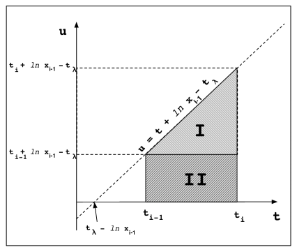
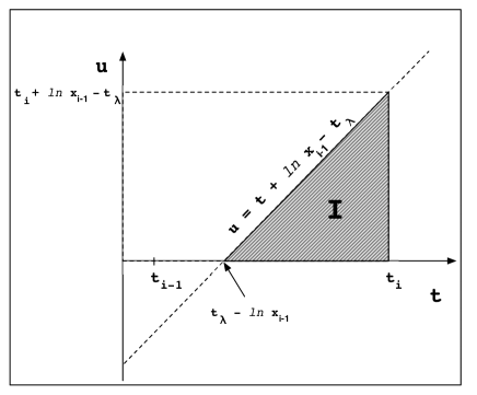
Figure 2: The integration domain in the $tu$ space for the case C’. Regions I (triangle) and II (rectangle) correspond to two integrals in eq. (53), respectively. Left frame: the case of ${t_{\lambda}-\ln x_{i-1}<t_{i-1}}$. Right frame: the case of ${t_{\lambda}-\ln x_{i-1}\geqslant t_{i-1}}$.

With the help of the rearrangement (53) we can calculate the virtual component

$$\Delta_{f}^{C^{\prime}} (t_{i},t_{i-1}|x_{i-1})=\Phi_{f}^{C^{\prime}}(t_{i},t_{i-1}|x_{i-1})-\bar{\Phi}_{f}^{C^{\prime}}(t_{i},t_{i-1}|x_{i-1})$$

$$= \int_{t_{i}}^{t_{i-1}}dt\int_{0}^{1}dz\theta_{(1-z)x_{i-1}>\lambda e^{-t}}\sum_{f^{\prime}}\biggl{(}\frac{\alpha_{S}(t+\ln x_{i-1}+\ln(1-z))}{2\pi}2z\bigl{(}P_{f^{\prime}f}^{R(0)}(z)-\bar{P}_{f^{\prime}f}^{R(0)}(z)\bigr{)}$$

$$+\Bigl{(}\frac{\alpha_{S}(t+\ln x_{i-1}+\ln(1-z))}{2\pi}\Bigr{)}^{2}2zP_{f^{\prime}f}^{R(1)C^{\prime}}(z)\biggr{)}$$

$$= \int_{t_{i-1}+\ln x_{i-1}-t_{\lambda}}^{t_{i}+\ln x_{i-1}-t_{\lambda}}due^{-u}2z\sum_{f^{\prime}}\Biggl{(}\frac{J_{1}(t_{i}+\ln x_{i-1},u)-J_{1}(u+t_{\lambda},u)}{2\pi}\bigl{(}P_{f^{\prime}f}^{R(0)}(z)-\bar{P}_{f^{\prime}f}^{R(C^{\prime})}(z)\bigr{)}$$

$$+\frac{J_{2}(t_{i}+\ln x_{i-1},u)-J_{2}(u+t_{\lambda},u)}{4\pi^{2}}P_{f^{\prime}f}^{R(1)C^{\prime}}(z)\Biggr{)}$$

$$+\theta_{t_{\lambda}-\ln x_{i-1}<t_{i-1}}\int_{0}^{t_{i-1}+\ln x_{i-1}-t_{\lambda}}due^{-u}2z\sum_{f^{\prime}}$$

$$\biggl{(}\frac{J_{1}(t_{i}+\ln x_{i-1},u)-J_{1}(t_{i-1}+\ln x_{i-1},u)}{2\pi}\bigl{(}P_{f^{\prime}f}^{R(0)}(z)-\bar{P}_{f^{\prime}f}^{R(C^{\prime})}(z)\bigr{)}$$

$$+\frac{J_{2}(t_{i}+\ln x_{i-1},u)-J_{2}(t_{i-1}+\ln x_{i-1},u)}{4\pi^{2}}P_{f^{\prime}f}^{R(1)C^{\prime}}(z)\biggr{)},\;\;\;\;z=1-e^{-u}.$$ (54)

Finally, the formula for the global weight, corresponding to eq. (36), in the case C’ reads

$$w^{(n)(C^{\prime})}=e^{-\Delta_{f_{n}}^{C^{\prime}}(t,t_{n}|x_{n})}\prod_{i=1}^{n}\left(\frac{\mathcal{K}^{R(C^{\prime})}_{f_{i}f_{i-1}}(t_{i},x_{i},x_{i-1})}{\bar{\mathcal{K}}^{R(C^{\prime})}_{f_{i}f_{i-1}}(t_{i},x_{i},x_{i-1})}e^{-\Delta_{f_{i-1}}^{C^{\prime}}(t_{i},t_{i-1}|x_{i-1})}\right).$$ (55)

4.2 Auxiliary algorithm

Similarly to the case B’, the second algorithm is based on the version of the simplified kernel (47) in which the coupling constant is taken in the LO approximation:

$$x\bar{\mathcal{K}}^{R(C^{\prime})(2)}_{f^{\prime}f}(t,x,w)\equiv \frac{\alpha_{LO}(t+\ln w+\ln(1-z))}{2\pi}2z\bar{P}^{R(C^{\prime})}_{f^{\prime}f}(z)\theta_{(1-z)w>\lambda e^{-t}}.$$ (56)

As in the case B’, in analogy to eq. (49), the Sudakov form factor becomes

$$\bar{\Phi}_{f}^{C^{\prime}(2)} (t_{i},t_{i-1}|x_{i-1})=\int_{t_{i-1}}^{t_{i}}dt\int_{0}^{1}d\Bigl{(}\frac{x}{x_{i-1}}\Bigr{)}\sum_{f^{\prime}}x\bar{\mathcal{K}}^{R(C^{\prime})(2)}_{f^{\prime}f}(t,x,x_{i-1})$$

$$= \frac{1}{\pi}\int_{t_{i-1}}^{t_{i}}dt\int^{t+\ln x_{i-1}-t_{\lambda}}_{0}du\alpha_{LO}(t-u)\biggl{(}A_{ff}^{(0)}+\sum_{f^{\prime}}\Bigl{(}\max_{z}F^{(0)}_{f^{\prime}f}(z)+M_{f^{\prime}f}\Bigr{)}\biggr{)}$$

$$= \int_{t_{i-1}}^{t_{i}}dt\Bigl{(}\rho_{LO}(t+\ln x_{i-1},t+\ln x_{i-1}-t_{\lambda})-\rho_{LO}(t+\ln x_{i-1},0)\Bigr{)}$$

$$\biggl{(}A_{ff}^{(0)}+\sum_{f^{\prime}}\Bigl{(}\max_{z}F^{(0)}_{f^{\prime}f}(z)+M_{f^{\prime}f}\Bigr{)}\biggr{)}$$

$$= \Bigl{(}\bar{\zeta}_{LO}(t_{i}+\ln x_{i-1})-\bar{\zeta}_{LO}(t_{i-1}+\ln x_{i-1})\Bigr{)}\biggl{(}A_{ff}^{(0)}+\sum_{f^{\prime}}\Bigl{(}\max_{z}F^{(0)}_{f^{\prime}f}(z)+M_{f^{\prime}f}\Bigr{)}\biggr{)},$$ (57)

where

$$\rho_{LO}(t+\ln x_{i-1},u) =\frac{1}{\pi}\int du\,\alpha_{LO}(t+\ln x_{i-1}-u)=-\frac{2}{\beta_{0}}\ln(2G(t+\ln x_{i-1},u)).$$ (58)

In order to generate $t_{i}$ the function $\bar{\zeta}_{LO}(t_{i}+\ln x_{i-1})$ is then inverted either analytically or as a test option also numerically.

The generation of the flavor index $f_{i}$ is based on the probability $p_{f_{i}}$ identical to eqs. (25) and (41)

The generation of the $z$-variable is based on the LO analogue of eq. (4.1)

$$dz_{i}p^{C^{\prime}(2)}(z_{i})= dz_{i}\frac{\alpha_{LO}(t_{i}+\ln x_{i-1}+\ln(1-z_{i}))}{\pi}\frac{\Theta_{(1-z_{i})x_{i-1}>\lambda e^{-t_{i}}}}{1-z_{i}}$$

$$\biggl{(}\int_{0}^{1}dz\frac{\alpha_{LO}(t_{i}+\ln x_{i-1}+\ln(1-z))}{\pi}\frac{\Theta_{(1-z)x_{i-1}>\lambda e^{-t_{i}}}}{1-z}\biggr{)}^{-1}$$

$$= du_{i}\partial_{u_{i}}\rho_{LO}(t_{i}+\ln x_{i-1},u_{i})\Theta_{t_{i}+\ln x_{i-1}-t_{\lambda}>u_{i}>0}$$

$$\Bigl{(}\rho_{LO}(t_{i}+\ln x_{i-1},t_{i}+\ln x_{i-1}-t_{\lambda})-\rho_{LO}(t_{i}+\ln x_{i-1},0)\Bigr{)}^{-1}.$$ (59)

As in the case B’, the whole NLO effect is introduced through the global weight. The virtual part of this weight, constructed on the base of the exact Sudakov form factor derived for the previous algorithm, follows from eq. (54)

$$\Delta_{f}^{C^{\prime}(2)} (t_{i},t_{i-1}|x_{i-1})=\Phi_{f}^{C^{\prime}}(t_{i},t_{i-1}|x_{i-1})-\bar{\Phi}_{f}^{C^{\prime}(2)}(t_{i},t_{i-1}|x_{i-1})$$

$$= \int_{t_{i}}^{t_{i-1}}dt\int_{0}^{1}dz\theta_{(1-z)x_{i-1}>\lambda e^{-t}}\sum_{f^{\prime}}\biggl{(}\frac{\alpha_{NLO}(t+\ln x_{i-1}+\ln(1-z))}{2\pi}2zP_{f^{\prime}f}^{R(0)}(z)$$

$$+\Bigl{(}\frac{\alpha_{NLO}(t+\ln x_{i-1}+\ln(1-z))}{2\pi}\Bigr{)}^{2}2zP_{f^{\prime}f}^{R(1)C^{\prime}}(z)$$

$$-\frac{\alpha_{LO}(t+\ln x_{i-1}+\ln(1-z))}{2\pi}2z\bar{P}_{f^{\prime}f}^{R(0)}(z)\biggr{)},$$ (60)

leading to

$$\Delta_{f}^{C^{\prime}(2)} (t_{i},t_{i-1}|x_{i-1})=$$

$$= \int_{t_{i-1}+\ln x_{i-1}-t_{\lambda}}^{t_{i}+\ln x_{i-1}-t_{\lambda}}due^{-u}2z\sum_{f^{\prime}}\biggl{(}-\frac{(J_{1}^{LO}(t_{i}+\ln x_{i-1},u)-J_{1}^{LO}(u+t_{\lambda},u))}{2\pi}\bar{P}_{f^{\prime}f}^{R(C^{\prime})}(z)$$

$$+\frac{(J_{1}(t_{i}+\ln x_{i-1},u)-J_{1}(u+t_{\lambda},u))}{2\pi}P_{f^{\prime}f}^{R(0)}(z)+\frac{(J_{2}(t_{i}+\ln x_{i-1},u)-J_{2}(u+t_{\lambda},u))}{4\pi^{2}}P_{f^{\prime}f}^{R(1)C^{\prime}}(z)\biggr{)}$$

$$+\theta_{t_{\lambda}-\ln x_{i-1}<t_{i-1}}\int_{0}^{t_{i-1}+\ln x_{i-1}-t_{\lambda}}due^{-u}2z$$

$$\sum_{f^{\prime}}\biggl{(}-\frac{(J_{1}^{LO}(t_{i}+\ln x_{i-1},u)-J_{1}^{LO}(t_{i-1}+\ln x_{i-1},u))}{2\pi}\bar{P}_{f^{\prime}f}^{R(C^{\prime})}(z)$$

$$+\frac{(J_{1}(t_{i}+\ln x_{i-1},u)-J_{1}(t_{i-1}+\ln x_{i-1},u))}{2\pi}P_{f^{\prime}f}^{R(0)}(z)$$

$$+\frac{(J_{2}(t_{i}+\ln x_{i-1},u)-J_{2}(t_{i-1}+\ln x_{i-1},u))}{4\pi^{2}}P_{f^{\prime}f}^{R(1)C^{\prime}}(z)\biggr{)},\;\;\;\;z=1-e^{-u}.$$ (61)

As a result, the complete formula for the global weight relevant for this algorithm reads

$$w^{(n)(C^{\prime})(2)}=e^{-\Delta_{f_{n}}^{C^{\prime}(2)}(t,t_{n}|x_{n})}\prod_{i=1}^{n}\left(\frac{\mathcal{K}^{R(C^{\prime})}_{f_{i}f_{i-1}}(t_{i},x_{i},x_{i-1})}{\bar{\mathcal{K}}^{R(C^{\prime})(2)}_{f_{i}f_{i-1}}(t_{i},x_{i},x_{i-1})}e^{-\Delta_{f_{i-1}}^{C^{\prime}(2)}(t_{i},t_{i-1}|x_{i-1})}\right).$$ (62)

5 Numerical results

In this Section we present numerical results obtained with the MC program EvolFMC version 2. The first version of this program has been presented in the Ref. [18] for the case of standard DGLAP LO evolution. Subsequently, the NLO evolution has been added in Ref. [19] and the LO modified-DGLAP evolution in Ref. [30]. The presented here EvolFMC v.2 includes three of the described above four algorithms for NLO modified-DGLAP evolution (the auxiliary algorithm for the B’ evolution is not implemented at the moment). In order to accommodate these new evolution schemes, the overall structure of the program has been modified, see Ref. [39] for details. As a result, it was important to perform a number of technical comparisons of the new code in order to establish its technical precisions. We very briefly describe these tests in the following subsection. Later on we present numerical results regarding the actual new evolution schemes. Before showing the results we discuss the choice of the counter terms and we list the input parameters.

5.1 Removal of the double counting

As indicated in Section 2, modification of the argument of the coupling constant in the evolution kernels is equivalent to adding some higher order (i.e. NLO and higher) terms. Therefore, one has to make sure that there is no double counting with the NLO part of the kernel. In the implementation presented here we follow the approach as discussed in Ref. [34]. Namely, we take the expansion of the $\alpha_{NLO}(t)$ in the form

$$\alpha_{NLO}(t+\ln\phi)=\alpha_{NLO}(t)-\frac{\beta_{0}}{2\pi}\alpha_{NLO}^{2}(t)\ln\phi+{\cal O}(1/t^{3}),$$ (63)

where $\phi$ represents any arbitrary change in the argument. Then the extra term in the kernels is of the form

$$-{\beta_{0}}\ln\phi\Bigl{(}\frac{\alpha_{NLO}(t)}{2\pi}\Bigr{)}^{2}2zP_{f^{\prime}f}^{R(0)}(z)\simeq-{\beta_{0}}\ln\phi\Bigl{(}\frac{\alpha_{NLO}(t+\ln\phi)}{2\pi}\Bigr{)}^{2}2zP_{f^{\prime}f}^{R(0)}(z)+{\cal O}(1/t^{3}),$$ (64)

and consequently the counter terms from eqs. (12) could be defined as follows

$$\Delta P_{f^{\prime}f}^{R(1)B^{\prime}}(z)={\beta_{0}}\ln(1-z)P_{f^{\prime}f}^{R(0)}(z),\;\;\;\hbox{for scheme B'},$$ (65)

$$\bar{\Delta}P_{f^{\prime}f}^{R(1)C^{\prime}}(z)={\beta_{0}}\bigl{(}\ln w+\ln(1-z)\bigr{)}P_{f^{\prime}f}^{R(0)}(z),\;\;z=x/w,\;\;\;\hbox{for scheme C'. }$$ (66)

However, a more detailed inspection of eq. (66) reveals that this formula over-subtracts the double counting. Namely, in the DGLAP evolution the kernels are functions of “local” $z$-variables only. In eq. (66) there is a corresponding $\ln(1-z)$ term. The other term, the $\ln w$, interconnects two emissions, and as such it is of genuinely beyond-DGLAP origin. It means that it is absent in the DGLAP kernel and there is no reason to remove it. As a result, the counter term in the C’ case becomes identical to the counter term in the B’ case. In the following we will present results for both variants in the C’ case, with the understanding that the preferred choice is the

$$\Delta P_{f^{\prime}f}^{R(1)B^{\prime}}(z)=\Delta P_{f^{\prime}f}^{R(1)C^{\prime}}(z)={\beta_{0}}\ln(1-z)P_{f^{\prime}f}^{R(0)}(z),$$ (67)

for both schemes B’ and C’.

5.2 Input parameters

The set-up of the EvolFMC code is the same for all the presented results. We use the gluon ($G$) and quark singlet ($Q$) PDFs with three massless quarks

$$D_{Q}=\sum_{i}\Bigl{(}D_{q_{i}}+D_{\bar{q}_{i}}\Bigr{)}.$$ (68)

As the initial distributions of the evolution we take

$$\begin{split}D^{0}_{G}(x)&=1.908\cdot x^{-1.2}(1-x)^{5.0},\\ D^{0}_{sea}(x)&=0.6733\cdot x^{-1.2}(1-x)^{7.0},\\ D^{0}_{u_{val}}(x)&=2.187\cdot x^{-0.5}(1-x)^{3.0},\\ D^{0}_{d_{val}}(x)&=1.230\cdot x^{-0.5}(1-x)^{4.0}\end{split}$$ (69)

and

$$\begin{split}D^{0}_{u}(x)&=D^{0}_{u_{val}}(x)+\frac{1}{6}D^{0}_{sea}(x),\\ D^{0}_{d}(x)&=D^{0}_{d_{val}}(x)+\frac{1}{6}D^{0}_{sea}(x),\\ D^{0}_{s}(x)&=D^{0}_{\bar{u}}(x)=D^{0}_{\bar{d}}(x)=D^{0}_{\bar{s}}(x)=\frac{1}{6}D^{0}_{sea}(x),\\ D^{0}_{Q}(x)&=D^{0}_{sea}(x)+D^{0}_{u_{val}}(x)+D^{0}_{d_{val}}(x).\end{split}$$ (70)

The QCD constant $\Lambda_{0}=0.2457$, the cut-off $\lambda=1$ GeV, $N_{f}=3$ and the dummy parameter $\eta=0.1$.

5.3 Technical tests

We have performed three different sets of the technical comparisons of the code EvolFMC v.2:

1. With the semianalytical code APCheb40 [45, 42] based on the expansion in Chebyshev polynomials.

2. With the previous version of the EvolFMC code: the EvolFMC v.1, which was extensively tested in the past.

3. Between different algorithms within the EvolFMC v.2. It is the most important test of the new NLO modified-DGLAP evolutions, which are not available in any other code.

The overall conclusion of all the tests is that the technical precision of the program EvolFMC v.2 is at least $5\times 10^{-4}$ (half of a per mille). For the details of the tests we refer the reader to Ref. [39].

5.4 Comparison of evolutions

Having established the technical precision of the EvolFMC code let us now proceed with the comparison of the various evolutions discussed earlier. Before getting into details let us remind the reader that in this paper for all of the results (i.e. for all of the evolutions) we use the same parameter setup: the same initial distributions at $Q=1$ GeV and the same $\Lambda_{0}$. In a more realistic study one should perform fits to the experimental data for each of the evolutions separately and then use different initial distributions for each evolution.

We organize the numerical comparisons in the following way: We begin by showing the ”reference” result, i.e. the standard DGLAP in the LO and NLO approximations (Fig. 3). Next, we show the new results for the B’-type and C’-type evolutions. These two plots (Figs.  4 and 5) are the main numerical results of this paper, showing the NLO corrections in the modified DGLAP evolutions. The next two plots (Figs. 6 and 7) are of technical character and show in a more detail certain aspects of the C’-type evolution. We conclude the section by comparing in a common plot all three evolutions in the NLO approximation (Fig. 8).

5.4.1 NLO versus LO

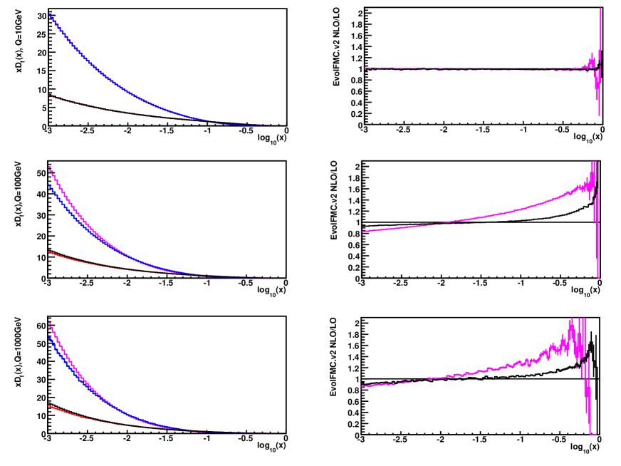
Figure 3: Left frames: the DGLAP-type evolutions in the LO and NLO approximations. Upper curves (LO: magenta and NLO: blue): the gluon $xD_{G}(x)$ distr.; lower curves (LO: black and NLO: red): the quark $xD_{Q}(x)$ distr. Right frames: the ratio of the NLO to LO distributions for the gluon (magenta) and quark (black) distributions. Top frames: the evolution up to 10 GeV. Bottom frames: the evolution up to 100 GeV.

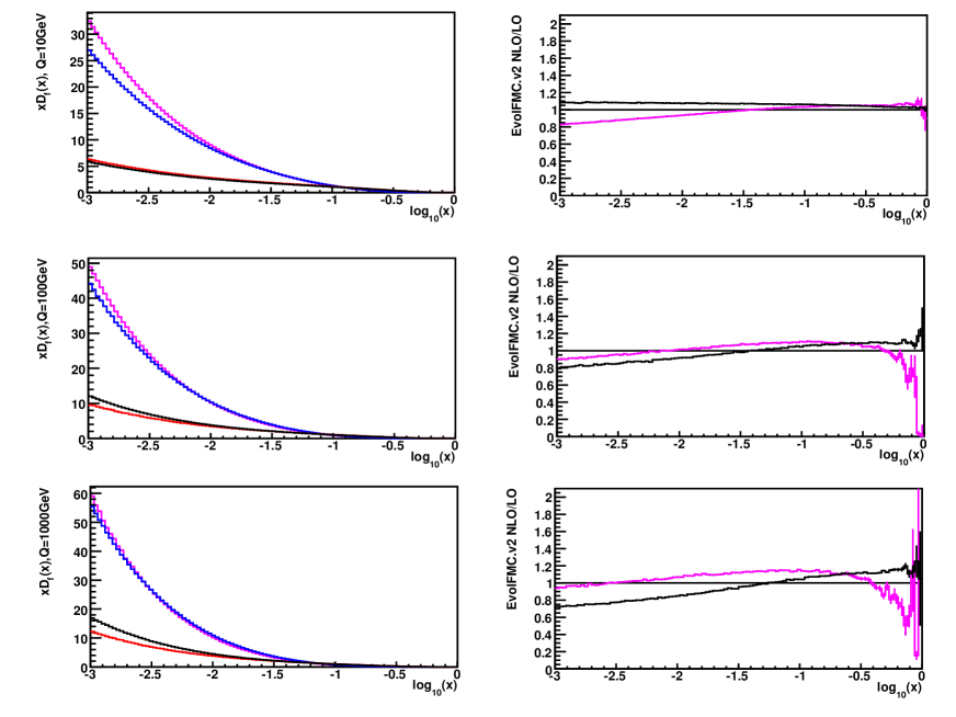
Figure 4: Left frames: the modified-DGLAP B’-type evolutions in the LO and NLO approximations. Upper curves (LO: magenta and NLO: blue): the gluon $xD_{G}(x)$ distr.; lower curves (LO: black and NLO: red): the quark $xD_{Q}(x)$ distr. Right frames: the ratio of the NLO to LO distributions for the gluon (magenta) and quark (black) distributions. Top frames: the evolution up to 10 GeV. Bottom frames: the evolution up to 100 GeV.

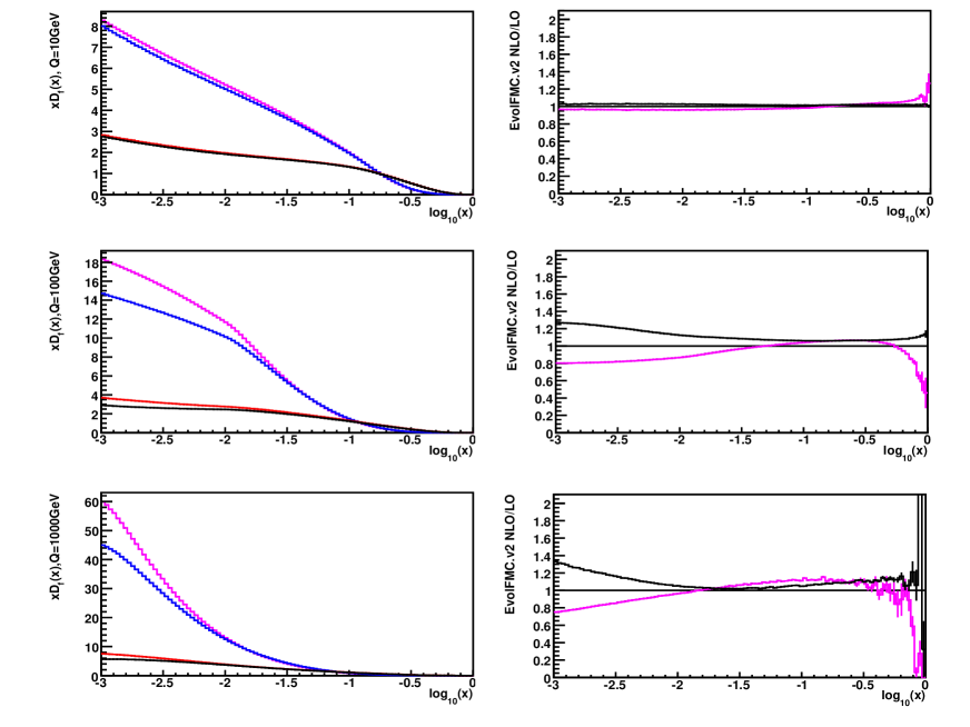
Figure 5: Left frames: the modified-DGLAP C’-type evolutions in the LO and NLO approximations. Upper curves (LO: magenta and NLO: blue): the gluon $xD_{G}(x)$ distr.; lower curves (LO: black and NLO: red): the quark $xD_{Q}(x)$ distr. Right frames: the ratio of the NLO to LO distributions for the gluon (magenta) and quark (black) distributions. Top frames: the evolution up to 10 GeV. Central frames: the evolution up to 100 GeV. Bottom frames: the evolution up to 1000 GeV.

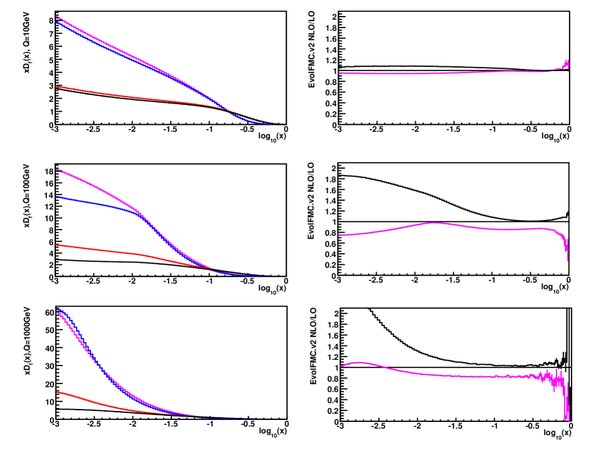
Figure 6: Left frames: the modified-DGLAP C’-type evolutions in the LO and NLO approximations with the modified disfavoured (C’-type) counter term. Upper curves (LO: magenta and NLO: blue): the gluon $xD_{G}(x)$ distr.; lower curves (LO: black and NLO: red): the quark $xD_{Q}(x)$ distr. Right frames: the ratio of the NLO to LO distributions for the gluon (magenta) and quark (black) distributions. Top frames: the evolution up to 10 GeV. Central frames: the evolution up to 100 GeV. Bottom frames: the evolution up to 1000 GeV.

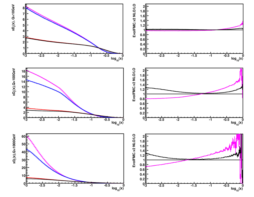
Figure 7: Left frames: the modified-DGLAP C’-type evolutions in the LO and NLO approximations without the counter term. Upper curves (LO: magenta and NLO: blue): the gluon $xD_{G}(x)$ distr.; lower curves (LO: black and NLO: red): the quark $xD_{Q}(x)$ distr. Right frames: the ratio of the NLO to LO distributions for the gluon (magenta) and quark (black) distributions. Top frames: the evolution up to 10 GeV. Central frames: the evolution up to 100 GeV. Bottom frames: the evolution up to 1000 GeV.

The ”reference” DGLAP evolution. In the Fig. 3 we show the case of the standard DGLAP. We show these well known results because DGLAP will serve us as a reference point in discussing the modified evolutions of the B’- and C’-type. We present the gluon and quark momentum distributions in LO and NLO approximations as well as their ratios. Three evolution time limits are shown: 10, 100 and 1000 GeV. The characteristic feature of the plots is that DGLAP NLO corrections are systematically bigger in the large $x$ region and they show the tendency of diverging in the $x\to 1$ limit. In the small $x$ region the NLO corrections are small. Results for the other evolutions will be presented in a similar way.
The B’-type evolution is shown in the Fig. 4. It is one of the two main new numerical results of this paper. As compared to the DGLAP case we can notice that the NLO corrections are a bit bigger in the small $x$ region, of the size up to 20%. In the large $x$ region, on the contrary, the corrections are much smaller and showing less divergent behavior. This is in agreement with the general principle of discussed here modifications of the DGLAP equation. These modifications are supposed to improve the description of the emission of soft partons [23, 26, 28] and it is the $x\to 1$ limit which corresponds to the limit of only soft emissions.
The C’-type evolution. In the Fig. 6 we compare the LO and NLO evolutions in the case of modified-DGLAP C’-type. We consider this figure as the most important new numerical result of this paper. We show the gluon and quark momentum distributions for two evolution time limits: 10, 100 and 1000 GeV. We see that at 100 and 1000 GeV the NLO corrections in the small-$x$ region are somewhat bigger than in the case B’, reaching even 30%. In the large $x$ region the NLO corrections seem to be even milder and slightly less divergent than in the B’ case, showing the same improvement over DGLAP. For the shorter time of 10 GeV the effects are much smaller. In fact, in this evolution type, due to the cut-off ${k_{T}>\lambda}$, much less of the evolution happens before 10 GeV, and both the LO and NLO curves are close to the initial condition as well as to each other. Note that in the case of both DGLAP and B’, the evolution at 10 GeV is already well developed. In order to reduce the evolution and get closer to the initial condition, in the DGLAP and B’ cases the evolution time must be much shorter, below 2 GeV at least.
Technical details related to C’-type evolution:
The C’-type evolution with the disfavoured counter term $\bar{\Delta}P$ from eq. (66). For the sake of comparison, in the Fig. 6, we present also the other, disfavored, choice of the counter term in the C’ evolution, given in eq. (66). The plots clearly confirm that the NLO corrections are much bigger, and, in addition, strongly divergent in the small $x$ limit.
The C’-type evolution with no counter term. As the last exercise, in Fig. 7, we completely switched off the counter term in the C’-type evolution. This way we try to understand better what actually causes the changes in the shape of the NLO corrections in the modified schemes: is it the genuine change of the argument of the coupling constant or rather the cut-off $\lambda$? In a crude approximation the counter term can be regarded as an estimate of the size of the pure effect of shifting the argument in the coupling constant. As one can see, the shapes in the right hand side plots in Fig. 7 have changed significantly in the large $x$ region, and have remained similar in the small $x$ region, as compared to the complete C’ plots from Fig. 5. This demonstrates that indeed it is the change of the argument that drives the effect in the region of soft emission. On the other hand, from the comparison of Figs. 5 and 7 to the DGLAP evolution, Fig. 3, we inferr that the higher order terms, resumed in the coupling constant, contribute as much as the counter term.
Remark on the small $x$ limit of the C’-evolution. As we have mentioned, C’ evolution is motivated by the CCFM equation. This equation treats the $x\to 0$ limit in a better way than the DGLAP equation, in a sense interpolating between DGLAP and BFKL equations. However, apart from the modifications in the coupling constant and the angular ordering, which we have incorporated in the C’ scheme, there is one more ingredient missing in C’ – the ’non-Sudakov’ form factor. This non-local form factor strongly modifies the small $x$ evolution. It depends on the transverse momenta of all the emitted partons. It is in principle not difficult to include such an effect into the Monte Carlo evolution of the C’-type by means of the rejection mechanism, provided the transverse momenta are properly generated within the cascade, and we plan to do it in the future [39].

Let us summarize the comparisons: 1. The modifications of the argument of the coupling constant decrease the size of the NLO corrections and reduce the divergences in the large $x$ region. 2. The NLO corrections in schemes B’ and C’ are significant, up to 30% in small $x$ region and must be included in the MC parton showers for the LHC. 3. One must remember, however, that these comparisons are to some degree artificial because, as discussed earlier, we use the same input PDF distributions for all evolution types. In a more complete study each of the evolutions should be separately fitted to the experimental data and obtained this way different input PDF distributions should be used.

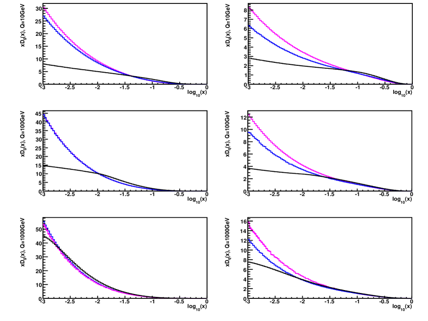
Figure 8: Comparison of three NLO evolutions: DGLAP (magenta), B’-type (blue) and C’-type (black). Left frames: the gluon $xD_{G}(x)$ distr. Right frames: the quark $xD_{Q}(x)$ distr. Top frames: the evolution up to 10 GeV. Central frames: the evolution up to 100 GeV. Bottom frames: the evolution up to 1000 GeV.

5.4.2 Different evolutions

As the last exercise we compare the three analyzed types of the evolution. In the Fig. 8 we show simultaneously all three evolutions in the NLO approximation. It is clearly visible that the difference between DGLAP and B’-type evolution (with $\alpha(Q(1-z))$) is rather small and of the quantitative form. On the contrary, the C’-type evolution (with $\alpha(k_{T})$) looks very different, both in the shape and in the magnitude. There is a visible flattening of the C’-type distributions around the value of $x\sim\lambda/Q$ caused by the cut-off $\lambda$. This follows from the condition $x_{i-1}(1-z_{i})\geq\lambda/Q$ which stops any cascade as soon as the $x_{i}$ variable falls below the $\lambda/Q$ threshold. In particular no evolution at all can develop for any $x_{0}\leq\lambda/Q$.

6 Summary and outlook

In this paper we have presented a series of Markovian MC algorithms that solve the QCD evolutions of the modified-DGLAP type in the NLO approximation. One of the two discussed modifications of the DGLAP evolution is of high practical importance. In this evolution, as the argument of the coupling constant the transverse momentum of the emitted parton is used, and the evolution time is identified with the rapidity variable. Such a modification is known to describe better the emission of soft partons. It can serve as a first step towards incorporating the complete CCFM effects into the evolution as well. In this paper we have called this scenario the C’-type evolution. The other scenario, called throughout the paper the B’-type evolution, uses $Q(1-z)$ as the argument of the coupling constant, modelling the ”one-loop” CCFM evolution equation. It is one of many possible $z$-dependent modifications of the argument discussed in the literature. Proper counter terms have been added to the evolution kernels in order to remove double counting at the NLO level.

The algorithms have been implemented into the new version of the MC program EvolFMC and extensively tested by comparisons with the semianalytical code APCheb40, with the previous version of EvolFMC and by comparisons of independent algorithms within the new version of EvolFMC itself. As the overall conclusion of the tests we claim the technical precision of the EvolFMC to be at least $5\times 10^{-4}$.

The comparison of the modified-DGLAP evolutions at both LO and NLO level shows that the NLO corrections are in general smaller in the modified evolutions and more importantly, the divergent behavior of the NLO corrections in the large $x$ region is limited, as expected. The only exception is the very low $x$ region where the NLO corrections in the modified schemes are larger. This is however the region where the DGLAP equation becomes less accurate anyway.

Quantitatively, the NLO corrections are relatively modest: in the B’ case they are small, of the order of up to 20% of the LO terms. For the $k_{T}$-dependent evolution (C’) they are, in most of the parameter space, of the order of 10%, but in some limited regions of small $x$ they grow up to 30%. These results, on the one hand, show that the NLO contributions are numerically significant and should be taken into account in the construction of the parton shower MC for the LHC experiments. This is especially important in the case of the physically well motivated $k_{T}$-dependent evolution. On the other hand, the convergence of the QCD perturbative expansion looks reasonably well, better than in the DGLAP case.

The main limitations of the presented in this paper MC algorithms are: missing effects due to the non-zero masses of the quarks in all of the discussed types of evolution and lack of the dedicated fits to the data for the modified-DGLAP type evolutions. Another interesting development line of the modified-DGLAP type evolutions would be to include a non-perturbative parametrization of the behavior of the coupling constant below the Landau pole. We hope to address some of these issues in the future.

7 Acknowledgments

The authors would like to thank S. Jadach, K. Golec-Biernat and Z. Was for numerous discussions and comments.

References

• [1] S. Moch, J. A. M. Vermaseren, and A. Vogt, Nucl. Phys. B688, 101 (2004), hep-ph/0403192.
• [2] A. Vogt, S. Moch, and J. A. M. Vermaseren, Nucl. Phys. B691, 129 (2004), hep-ph/0404111.
• [3] C. Anastasiou, K. Melnikov, and F. Petriello, Nucl. Phys. B724, 197 (2005), hep-ph/0501130.
• [4] M. Grazzini, (2008), arXiv:0801.3232.
• [5] A. Gehrmann-De Ridder, T. Gehrmann, E. W. N. Glover, and G. Heinrich, JHEP 12, 094 (2007), arXiv:0711.4711.
• [6] T. Sjostrand, S. Mrenna, and P. Skands, (2007), arXiv:0710.3820.
• [7] T. Sjostrand et al., Comput. Phys. Commun. 135, 238 (2001), hep-ph/0010017.
• [8] S. Gieseke et al., (2006), hep-ph/0609306.
• [9] G. Corcella et al., JHEP 01, 010 (2001), hep-ph/0011363.
• [10] L. Lonnblad, Comput. Phys. Commun. 71, 15 (1992).
• [11] S. Frixione and B. R. Webber, JHEP 06, 029 (2002), hep-ph/0204244.
• [12] P. Nason, JHEP 11, 040 (2004), hep-ph/0409146.
• [13] L.N. Lipatov, Sov. J. Nucl. Phys. 20 (1975) 95;
V.N. Gribov and L.N. Lipatov, Sov. J. Nucl. Phys. 15 (1972) 438;
G. Altarelli and G. Parisi, Nucl. Phys. 126 (1977) 298;
Yu. L. Dokshitzer, Sov. Phys. JETP 46 (1977) 64.
• [14] E. G. Floratos, D. A. Ross, and C. T. Sachrajda, Nucl. Phys. B129, 66 (1977).
• [15] E. G. Floratos, D. A. Ross, and C. T. Sachrajda, Nucl. Phys. B152, 493 (1979).
• [16] G. Curci, W. Furmanski, and R. Petronzio, Nucl. Phys. B175, 27 (1980).
• [17] W. Furmanski and R. Petronzio, Phys. Lett. B97, 437 (1980).
• [18] S. Jadach and M. Skrzypek, Acta Phys. Polon. B35, 745 (2004), hep-ph/0312355.
• [19] K. Golec-Biernat, S. Jadach, W. Placzek, and M. Skrzypek, Acta Phys. Polon. B37, 1785 (2006), hep-ph/0603031.
• [20] S. Jadach and M. Skrzypek, Comput. Phys. Commun. 175, 511 (2006), hep-ph/0504263.
• [21] S. Jadach, W. Placzek, M. Skrzypek, P. Stephens, and Z. Was, (2007), hep-ph/0703281.
• [22] T. Sjostrand, Phys. Lett. B157, 321 (1985).
• [23] D. Amati, A. Bassetto, M. Ciafaloni, G. Marchesini, and G. Veneziano, Nucl. Phys. B173, 429 (1980).
• [24] S. J. Brodsky, G. P. Lepage, and P. B. Mackenzie, Phys. Rev. D28, 228 (1983).
• [25] W. K. Wong, Phys. Rev. D54, 1094 (1996), hep-ph/9601215.
• [26] G. Sterman, Nucl. Phys. B281, 310 (1987).
• [27] B. I. Ermolaev, M. Greco, and S. I. Troyan, Phys. Lett. B522, 57 (2001), hep-ph/0104082.
• [28] B. I. Ermolaev and S. I. Troyan, Phys. Lett. B666, 256 (2008), 0805.2278.
• [29] M. Ciafaloni, Nucl. Phys. B296 (1988) 49;
S. Catani, F. Fiorani and G. Marchesini, Phys. Lett. B234 339, Nucl. Phys. B336 (1990) 18;
G. Marchesini, Nucl. Phys. B445 (1995) 49.
• [30] K. Golec-Biernat, S. Jadach, W. Placzek, P. Stephens, and M. Skrzypek, Acta Phys. Polon. B38, 3149 (2007), hep-ph/0703317.
• [31] M. Skrzypek, S. Jadach, K. Golec-Biernat, and W. Placzek, Acta Phys. Polon. B38, 2369 (2007).
• [32] G. Marchesini and B. R. Webber, Nucl. Phys. B349, 617 (1991).
• [33] J. Kwiecinski, Acta Phys. Polon. B33 (2002) 1809;
A. Gawron, J. Kwiecinski and W. Broniowski, Phys. Rev. D68 (2003) 054001;
A. Gawron, J. Kwiecinski, Phys. Rev. D70 (2004) 014003.
• [34] R. G. Roberts, Eur. Phys. J. C10, 697 (1999), hep-ph/9904317.
• [35] P. Stoklosa and M. Skrzypek, Acta Phys. Polon. B38, 2577 (2007).
• [36] S. Tsuno, T. Kaneko, Y. Kurihara, S. Odaka, and K. Kato, Comput. Phys. Commun. 175, 665 (2006), hep-ph/0602213.
• [37] Y. Kurihara et al., Nucl. Phys. B654, 301 (2003), hep-ph/0212216.
• [38] H. Jung and G. P. Salam, Eur. Phys. J. C19, 351 (2001), hep-ph/0012143.
• [39] S. Jadach et al., in preparation.
• [40] M. H. Seymour, Comp. Phys. Commun. 90, 95 (1995), hep-ph/9410414.
• [41] T. Sjostrand, S. Mrenna, and P. Skands, JHEP 05, 026 (2006), hep-ph/0603175.
• [42] K. Golec-Biernat, S. Jadach, W. Placzek, and M. Skrzypek, Acta Phys. Polon. B39, 115 (2008), 0708.1906.
• [43] W. Placzek, K. Golec-Biernat, S. Jadach, and M. Skrzypek, Acta Phys. Polon. B38, 2357 (2007), arXiv:0704.3344.
• [44] G. Marchesini and B. R. Webber, Nucl. Phys. B310, 461 (1988).
• [45] K. Golec-Biernat, APCheb40, the Fortran code available on the request from the author, unpublished.