Time evolution of the line emission from the inner circumstellar ring of SN 1987A and its hot spots

We present seven epochs between October 1999 and November 2007 of high resolution VLT/UVES echelle spectra of the ejecta-ring collision of SN 1987A.

The fluxes of most of the narrow lines from the unshocked gas decreased by a factor of $2-3$ during this period, consistent with the decay from the initial ionization by the shock break-out. However, [O III] in particular shows an increase up to day $\sim 6800$. This agrees with radiative shock models where the pre-shocked gas is heated by the soft X-rays from the shock. The evolution of the [O III] line ratio shows a decreasing temperature of the unshocked ring gas, consistent with a transition from a hot, low density component which was heated by the initial flash ionization to the lower temperature in the pre-ionized gas ahead of the shocks.

The line emission from the shocked gas increases rapidly as the shock sweeps up more gas. We find that the neutral and high ionization lines follow the evolution of the Balmer lines roughly, while the intermediate ionization lines evolve less rapidly. Up to day $\sim 6800$, the optical light curves have a similar evolution to that of the soft X-rays. The break between day $6500$ and day $7000$ for [O III] and [Ne III] is likely due to recombination to lower ionization levels. Nevertheless, the evolution of the [Fe XIV] line, as well as the lines from the lowest ionization stages, continue to follow that of the soft X-rays, as expected.

There is a clear difference in the line profiles between the low and intermediate ionization lines, and those from the coronal lines at the earlier epochs. This shows that these lines arise from regions with different physical conditions, with at least a fraction of the coronal lines coming from adiabatic shocks. At later epochs the line widths of the low ionization lines, however, increase and approach those of the high ionization lines of [Fe X-XIV]. The H$\alpha$ line profile can be traced up to $\sim 500\rm\leavevmode\nobreak\ km\leavevmode\nobreak\ s^{-1}$ at the latest epoch. This is consistent with the cooling time of shocks propagating into a density of $(1-4)\times 10^{4}\mbox{ cm}^{-3}$. This means that these shocks are among the highest velocity radiative shocks observed.

1 Introduction

Since the explosion more than two decades ago, supernova (SN) 1987A in the Large Magellanic Cloud (LMC) has been extensively observed in multiple wavelength ranges. It is now by far the most studied of all supernovae. A few months after outburst, the first evidence of the stationary circumstellar matter around the SN came from detection of narrow optical lines (Wampler et al. 1988) and UV emission lines by the International Ultraviolet Explorer (IUE) (Fransson et al. 1989). Resolved imaging observations later disclosed the now classical ring nebula around the SN consisting of three approximately plane-parallel rings; the radioactive SN debris is located at the center of the inner equatorial ring (ER). The ER is intrinsically close to circular in shape and has a tilt angle of $43^{\circ}$ (Sugerman et al. 2005; Kjær et al. 2007). The two outer rings (ORs) are displaced by $\sim 1.3\leavevmode\nobreak\ {\rm ly}$ (Sugerman et al. 2005) on either side of the ER ring plane (Crotts et al. 1989; Wampler et al. 1990; Burrows et al. 1995). The observed radii of the rings ($\sim 0.6\leavevmode\nobreak\ {\rm ly}$ for the ER), together with the measured radial expansion velocities ($\sim 10.3\rm\leavevmode\nobreak\ km\leavevmode\nobreak\ s^{-1}$ for the ER), indicate that the ring system was ejected about $20,000$ years ago, if constant expansion velocities of the rings are assumed. The formation mechanism of the three rings is still not fully understood, although a scenario is that the structure was formed as a result of a merger with a binary companion in a common envelope phase (Morris & Podsiadlowski 2007). However, single star models for the progenitor have also been proposed (e.g., Eriguchi et al. 1992; Woosley et al. 1997).

The ring structure was photoionized by the EUV and soft X-ray flash emitted from the SN explosion, and since then the gas has been cooling, recombining and fading roughly linearly with time (e.g., Lundqvist & Fransson 1996). This gas can be traced by narrow emission lines and the fading of these lines is consistent with ring gas densities in the range $3\times 10^{3}-3\times 10^{4}\rm\leavevmode\nobreak\ cm^{-3}$ (Lundqvist & Fransson 1996; Pun 2007). Early light echoes revealed, however, that the observed photoionized gas is probably only a small fraction of the total mass ejected from the progenitor system (Gouiffes et al. 1988; Crotts et al. 1989).

A new phase was entered, marking the birth of the SN remnant, as the SN debris drives a blast wave into its circumstellar medium. The first indication of the encounter between this blast wave and the ER came in 1997 from HST/STIS observations where broad ($\sim 250\rm\leavevmode\nobreak\ km\leavevmode\nobreak\ s^{-1}$) blue-shifted emission components were detected in H$\alpha$ (Sonneborn et al. 1998). Later it was found that this interaction could be detected in HST images already in 1995 (Lawrence et al. 2000). The interaction took place in a small region located in the northeastern part of the ER (P.A. $29^{\circ}$) (Pun et al. 1997). This “hot spot” is usually referred to as Spot 1. Hence, Spot 1 is believed to mark the place were the blast wave first strikes an inward-pointing protrusion of the ER surrounded by an H II region inside the ring (Pun et al. 2002). The protrusions are presumably a result of Rayleigh-Taylor instabilities caused by the interaction of the stellar progenitor wind with the ER. Since 1997, Spot 1 has steadily increased in flux and many more clumps have been shocked giving rise to more “hot spots” in different locations around the ring. Ten years later, there are “hot spots” distributed all around the ER. It is, however, not clear if the ring is really homogeneous, or if it may consist of isolated clumps. Time will tell.

In the interaction between the supernova ejecta and the circumstellar matter a multi-shock system develops. A forward shock (blast wave) propagates into the CSM and a reverse shock is driven backward (in the Lagrangian frame of reference) into the ejecta (Chevalier 1982). A complication is that the circumstellar structure is probably complex, with a constant density H II region inside the ER (Chevalier & Dwarkadas 1995). When the forward shock, propagating with a velocity of $\sim 3500\rm\leavevmode\nobreak\ km\leavevmode\nobreak\ s^{-1}$ through the circumstellar gas (with density $\sim 10^{2}\rm\leavevmode\nobreak\ cm^{-3}$), reaches the denser ER ($\sim 10^{4}{\rm\leavevmode\nobreak\ cm^{-3}}$), slower shocks are transmitted into the ring. Because the transmitted shock velocities depend on both the density profile of the ER and the incident angle, a wide range of shock velocities is expected ($\sim 10^{2}-10^{3}\rm\leavevmode\nobreak\ km\leavevmode\nobreak\ s^{-1}$) (Michael et al. 2002). In addition, the interaction with a density jump may create reflected shocks between the ring and the reverse shock.

The interaction has been observed in virtually all wavelength ranges, from radio to X-rays (e.g. McCray 2007). The high resolution X-ray spectrum observed by Chandra shows a number of H and He-like emission lines in the wavelength range $5-25$ Å such as Si XIII-XIV, Mg XI-XII, Ne IX-X, O VII-VIII, Fe XVII and N VII emitted by shocks produced by the interaction of the blast wave and the ER. The line profiles indicate gas velocities in the range $\sim 300-1700\rm\leavevmode\nobreak\ km\leavevmode\nobreak\ s^{-1}$ (Zhekov et al. 2005, 2006; Dewey et al. 2008). As the expanding ejecta collide with the CSM, the luminosity increases rapidly in radio synchrotron emission (Gaensler et al. 2007), as well as in X-rays originating from the hot shocked gas (Park et al. 2007). The ring evolution has also been studied in mid-IR (Bouchet et al. 2006), near-IR (Kjær et al. 2007), as well as optical and UV (Pun et al. 2002; Sugerman et al. 2002, 2005; Gröningsson et al. 2006, 2008).

For this paper, the X-rays are of special interest. Up to 1999 both the soft and hard X-rays correlated well with the radio emission. Since then, however, the flux of soft X-rays began to increase much more rapidly than both radio and hard X-ray fluxes (Park et al. 2007). Instead, in Gröningsson et al. (2006) we found that the evolution of the flux of the optical high ionization lines from the hot spots correlated well with the soft X-ray emission. This suggests that much of the soft X-ray emission arises from the ejecta-ring collision, while the hard X-rays mainly come from the hot gas between the reverse and the forward shock. The radio emission continues to correlate well with hard X-rays, and is most likely caused by relativistic electrons accelerated by the reverse shock interior to the ER (Zhekov et al. 2006).

A complementary view of the interaction is offered by the IR emission from the dust (Bouchet et al. 2006; Dwek et al. 2008). Dwek et al. find a temperature of the silicate rich dust of $\sim 180$ K, heated either by the shocked gas or by the radiation from the shocks. The dust emission coincides roughly with the optical emission. A surprising result is the comparatively low IR to X-ray ratio, indicating destruction of the dust by the shock. The fact that this ratio decreased with time is also consistent with dust destruction.

In this paper we discuss the evolution of the optical emission lines from high resolution spectroscopic data taken with VLT/UVES. In the first paper in this series (Gröningsson et al. 2006) we discussed the implications of the coronal lines from [Fe X-XIV] found in these spectra. In the second paper (Gröningsson et al. 2008, in the following referred to as G08) we discussed a full analysis of the spectrum from one epoch, 2002 October. These spectra showed narrow emission line components with FWHM $\sim 10-30\rm\leavevmode\nobreak\ km\leavevmode\nobreak\ s^{-1}$ for most of the lines, arising from the unshocked ring gas. The interaction between the ejecta and the ER can be seen as intermediate velocity lines coming from shocked ring material, extending to approximately $\pm 300\rm\leavevmode\nobreak\ km\leavevmode\nobreak\ s^{-1}$, with clearly asymmetric line profiles. In addition, a broad ($\sim 15,000\rm\leavevmode\nobreak\ km\leavevmode\nobreak\ s^{-1}$) velocity component in H$\alpha$ and [Ca II], originating from the reverse shock in the outer ejecta (Heng 2007), is clearly visible. In contrast to the analysis in G08, we focus in this paper on the time evolution of the line emission. Hence, in this paper, we present data taken with VLT at seven epochs ranging from 1999 October to 2007 November.

The observations and data reductions are discussed in Sect. 2. Analysis of the data is presented in Sect. 3 followed by discussions of the results in Sect. 4, and finally a summary in Sect. 5.

2 Observations

High resolution spectra of SN 1987A were obtained using the Ultraviolet and Visual Echelle Spectrograph (UVES) at ESO/VLT at Paranal, Chile (Dekker et al. 2000). The UVES spectrograph disperses the light beam in two separate arms covering different wavelength ranges of the spectrum. The blue arm covering the shorter wavelengths ($\sim 3030-4990$ Å) is equipped with a single CCD detector with a spatial resolution of $0\aas@@fstack{\prime\prime}246/\mathrm{pixel}$ while the red arm ($\sim 4760-10\,600$ Å) is covered by a mosaic of two CCDs having a resolution of $0\aas@@fstack{\prime\prime}182/\mathrm{pixel}$. Thus with two different dichroic settings the wavelength coverage is $\sim 3030-10\,600$ Å. Due to the CCD mosaic in the red arm there are, however, gaps at $5770-5830$ Å and $8540-8650$ Å. The spectral resolving power is $40\,000$ for a $1\aas@@fstack{\prime\prime}0$ wide slit.

Spectra of SN 1987A were obtained at 7 different epochs ranging from October 16 1999 to November 28 2007, henceforth referred to as Epochs 1–7. See Table 1 for the observational details. The observations were performed in service mode for Epochs 2–7 whereas Epoch 1 was part of the instrument “first light” program. For Epochs 2–7 a $0\aas@@fstack{\prime\prime}8$ wide slit was centered on the SN and with a position angle PA$=30^{\circ}$ (see Fig. 1). Hence, the spectral resolution for these epochs was $\lambda/\Delta\lambda\sim 50\,000$ which corresponds to a velocity of $6\rm\leavevmode\nobreak\ km\leavevmode\nobreak\ s^{-1}$. For Epoch 1 the slit width was $1\aas@@fstack{\prime\prime}0$ and rotated to PA$=20^{\circ}$.

Table 1: VLT/UVES observations of SN 1987A and its rings.

Epoch	Date	Days after	Setting	$\lambda$ range	Slit width	Resolution	Exposure	Seeing	Airmass
		explosion		(nm)	(arcsec)	$(\lambda/\Delta\lambda$)	(s)	(arcsec)
1	1999 Oct 16	4618	346+580	303–388	1.0	40,000	1,200	1.0	1.4
				476–684
2	2000 Dec 9–14	5039–5043	346+580	303–388	0.8	50,000	10,200	0.4–0.8	1.4
				476–684
		5038–5039	390+860	326–445			9,360	0.4	1.4–1.6
				660–1060
3	2002 Oct 4–7	5704–5705	346+580	303–388	0.8	50,000	10,200	0.7–1.0	1.5–1.6
				476–684
		5702–5703	437+860	373–499			9,360	0.4–1.1	1.4–1.5
				660–1060
4	2005 Mar 21	6601–6623	346+580	303–388	0.8	50,000	9,200	0.6–0.9	1.5–1.8
	Apr 8-12			476–684
		6621–6623	437+860	373–499			4,600	0.5	1.6–1.7
				660–1060
5	2005 Oct 20	6826	346+580	303–388	0.8	50,000	2,300	0.9	1.4
	Nov 1–12			476–684
		6814–6837	437+860	373–499			9,200	0.5–1.0	1.4–1.6
				660–1060
6	2006 Oct 1–29	7160–7180	346+580	303–388	0.8	50,000	9,000	0.5–0.9	1.4–1.5
	Nov 10–15			476–684
		7188–7205	437+860	373–499			9,000	0.5–1.0	1.4
				660–1060
7	2007 Oct 23–24	7547–7583	346+580	303–388	0.8	50,000	11,250	0.8–1.4	1.4–1.6
	Nov 27–28			476–684
		7547	437+860	373–499			9,000	1.1–1.4	1.4–1.6
				660–1060

For the data reduction we made use of the MIDAS implementation of the UVES pipeline version 2.0 for Epochs 1–3 and version 2.2 for Epochs 4–7. For a detailed description of the steps involved in the reductions we refer to G08.

For the time evolution of the fluxes an accurate absolute flux calibration is necessary. As discussed in Gröningsson et al. (2006) and G08, we estimated the accuracy of the flux calibration by comparing the spectra of flux-calibrated spectrophotometric standard stars with their tabulated physical fluxes. In addition, we compared emission line fluxes from different exposures (and hence with different atmospheric seeing conditions) within the same epochs. From these measurements, together with the results from HST photometry in Appendix A, we conclude that the accuracy in relative fluxes should be within $10-15\%$. The estimation of the absolute systematic flux error was done from a comparison between the UVES fluxes and HST spectra and photometry (see G08 and Appendix A). From this, together with our experience with such data, we estimate that the uncertainty of the absolute fluxes should be less than $20-30\%$.

We sampled the ring at the northeast and southwest positions (see Fig. 1). However, the limited spatial resolution of these observations makes it impossible to distinguish between different hot spots located on the same side of the ring and covered by the slit. Hence, we studied the HST images taken at roughly the same epochs (see Fig. 1 and Appendix) to identify the number of hot spots covered by the slit for both each epoch and side of the ring. For Epochs 1–2 we used images taken with the WFPC2 and narrow-band filter F656N. These images reveal that for Epoch 1 only Spot 1 contributes to the emission from the shocked gas over the entire ring. At Epoch 2 there are contributions from effectively two different spots at the northern side of the ring, even though Spot 1 clearly dominates. On the southern side, two spots have now appeared. For Epochs 3–6 we investigated images taken with the ACS instrument. These show that at Epoch 3 the shocked gas emission on the northern part now comes from four spots, while no new spots have appeared on the southern side. At Epochs 4–6 there are hot spots almost all around the ring, although the main contributions come from five spots on the northern side and four on the southern side of the ring. At these three epochs spot 1 appears not to be the strongest one on the northern side, although the first two spots to appear on the southern side are still strongest at Epoch 6. Unfortunately we have no comparable HST imaging for Epoch 7, and consequently no study of individual spots can be made for that epoch.

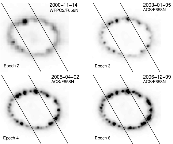
Figure 1: Ring images taken with HST at four different epochs (obtained by the SAINTS team; PI: R.P. Kirshner). The slit position of the VLT/UVES observations is superimposed (the slit width is $0\aas@@fstack{\prime\prime}8$ and $\rm{PA}=30^{\circ}$). North is up and east is to the left. All images except the earliest epoch (upper left panel) have the same scaling in flux. The epochs labeled in the panels correspond roughly to the time of the HST observations. Note the evolution and distribution of “hot spots” around the ring. The evolution is most prominent on the southwest part of the ring.

3 Analysis

3.1 Systemic velocity and ring expansion

The systemic velocity of SN 1987A can be estimated directly from the peak velocities of the unshocked gas. The best accuracy should in principle be obtained for the strongest emission lines with well defined intensity peaks, such as the [O II], [S II] and [N II] doublets. However, since there are uncertainties in the rest wavelengths and in the wavelength calibration (amounting to $\sim 0.01\mbox{ \AA}$, corresponding to $0.6\rm\leavevmode\nobreak\ km\leavevmode\nobreak\ s^{-1}$ at 5000 Å), we have chosen to include all lines in Tables LABEL:tab:narrowlines2–LABEL:tab:narrowlines7 in the velocity estimate. Taking the average of the peak velocities of the northern ($281.66\pm 0.07\rm\leavevmode\nobreak\ km\leavevmode\nobreak\ s^{-1}$) and southern ($291.81\pm 0.07\rm\leavevmode\nobreak\ km\leavevmode\nobreak\ s^{-1}$) parts of the ER in the data set we find a center of mass velocity of $286.74\pm 0.05\rm\leavevmode\nobreak\ km\leavevmode\nobreak\ s^{-1}$ ($1\sigma$ errors). This result is in agreement with Wampler & Richichi (1989) and Meaburn et al. (1995) who obtained $286.3\pm 0.8\rm\leavevmode\nobreak\ km\leavevmode\nobreak\ s^{-1}$ and $286.5\pm 1\rm\leavevmode\nobreak\ km\leavevmode\nobreak\ s^{-1}$, respectively, but lower than $287.6\pm 0.1\rm\leavevmode\nobreak\ km\leavevmode\nobreak\ s^{-1}$ and $289.2\rm\leavevmode\nobreak\ km\leavevmode\nobreak\ s^{-1}$ as reported by Cumming (1994) and Crotts & Heathcote (1991), respectively.

The expansion velocity of the ER is more difficult to measure directly from the data. One method to estimate the expansion velocity would be to assume a luminosity and a temperature distribution of the ER and then model the resulting line profiles of either side of the ER by taking into account the instrumental broadening, spectral resolution and atmospheric seeing (e.g., Meaburn et al. 1995). The best fit model to the narrow emission components would then give the expansion velocity. A more direct approach is to measure differences between the peak velocities of the emission lines from the unshocked gas at the north and south parts of the ER and correct for the ring inclination and the slit orientation. From geometrical considerations we would ideally have for the radial velocity

$$V_{r}={|\Delta V_{peak}|\over 2{\rm sin}(i){\rm cos}(\psi)}.$$ (1)

The angle $\psi$ is given by ${\rm tan}(\psi)={\rm tan}({\rm PA}+\phi){\rm cos}(i)$ where $i$ is the inclination angle of the ring, PA the position angle of the slit, and $\phi$ the angle between the minor axis of the ring and north. However, due to the slit width and the seeing, different parts of the ring contribute to the different components along the line of sight. Since the total broadening is a convolution of the macroscopic motion and the thermal motion, the peak of the emission line will be velocity shifted with an amount and a direction that depends on the skewness of the macroscopic velocity distribution, temperature and the atomic weight of the element. The velocity distribution of the northern part of the ring is expected to be positively skewed and the distribution at the southern part is expected to be negatively skewed. Hence, in this case the measured $\Delta V_{peak}$ would be systematically underestimated and, as a consequence, Eq. (1) only provides a lower limit to the radial velocity. To account for the fact that the emission lines sample a range of $\psi$’s, Eq. (1) can be multiplied by the factor $(\Delta\psi/2)/{\rm sin}(\Delta\psi/2)$. Comparing the width of the slit to the size of the ER, we estimate $\Delta\psi$ to be in the range $\sim 60^{\circ}-90^{\circ}$. Hence, it follows that Eq. (1) would underestimate the real expansion velocity by $\sim 5-10\%$.

To minimize the systematic errors, we chose to only include data from Epoch 2 (2000 Dec. Table LABEL:tab:narrowlines2). The observations at this epoch have the best seeing conditions (Table LABEL:tab:obslog) and least contamination of emission from the shocked ring gas. Furthermore, to reduce the systematic uncertainties due to temperature effects, we only included the emission lines from elements with a large atomic weight. The thermal broadening for these lines is very small compared to the macroscopic velocity distribution. Of course, we need to assume that these lines have roughly the same spatial luminosity distributions as the other lines around the ring. Therefore, we used the narrow components of the relatively strong [S II] $\lambda 4069+76,\lambda 6716+31$, [Ar III] $\lambda 7136$, [Fe II] $\lambda 7155$ and [Ca II] $\lambda 7324$ lines in Table LABEL:tab:narrowlines2 to estimate $\Delta V_{peak}$. If we adopt the geometrical values of the ER suggested by Sugerman et al. (2002, 2005), i.e., $i=43^{\circ}$ and $\phi=9.6^{\circ}$, we derive for $\mathrm{PA}=30^{\circ}$ the radial expansion velocity $V_{r}=10.3\pm 0.3\rm\leavevmode\nobreak\ km\leavevmode\nobreak\ s^{-1}$ ($1\sigma$ error). This result agree with earlier estimates by Cumming (1994) who found $10.3\pm 0.4\rm\leavevmode\nobreak\ km\leavevmode\nobreak\ s^{-1}$ and Crotts & Heathcote (2000) who reported $10.5\pm 0.3\rm\leavevmode\nobreak\ km\leavevmode\nobreak\ s^{-1}$.

3.2 Evolution of the unshocked components

As discussed in detail in G08 (see Table 2 in that paper), we detect narrow components for a large range of ionization stages, from neutral up to Ne V and Fe VII. The only exceptions are the coronal lines from Fe X-XIV.

Figure 2 shows the flux evolution of the narrow lines for the northern and southern parts of the ER (see Tables LABEL:tab:narrowlines2–LABEL:tab:narrowlines7). In order to compare the trends of the different lines more clearly we have normalized these to the flux on October 2002 (Epoch 3). Because of the low S/N, we do not include Epoch 1 in the analysis.

The Balmer line fluxes appear to be constant in time up to day $\sim 6800$, but after this epoch there is a clear decline. The fluxes from the low-ionization [N II], [O I], [O II], [S II] and [Fe II] lines roughly follow this trend. In contrast, the highly ionized [Ne III] and [O III] fluxes appear to increase up to day $\sim 6800$. After that they are constant or slowly decreasing. We return to this interesting result in Sect. 4.1. The fluxes of [Ne V] $\lambda 3426$ have a large statistical uncertainty, and it is therefore difficult to say anything regarding the trend.

Except for [Fe II], it is difficult to draw any conclusions from the other iron lines of higher ionization stage due to their large statistical uncertainties.

Figure 3 shows the width (FWHM) of the emission lines as a function of time for the northern part of the ER (see Tables LABEL:tab:narrowlines2–LABEL:tab:narrowlines7). The line widths of the narrow emission lines depend on the instrumental broadening ($\sim 6\rm\leavevmode\nobreak\ km\leavevmode\nobreak\ s^{-1}$), the bulk motion of the ER and the temperature of the unshocked gas. The instrumental broadening can be considered constant from epoch to epoch. The expansion velocity of the ring should also be fairly constant. However, due to the evolution of the spatial ring profile, different regions of the ring may be sampled in the extraction process causing slight changes in the macroscopic velocity distribution from epoch to epoch. This effect would in such case broaden the line and become more important for later epochs. Nevertheless, for the light elements, such as hydrogen and helium, any differences should be small relative to the thermal broadening, and the FWHM from epoch to epoch should mainly reflect changes in temperatures for these lines.

As shown in Fig. 3, the widths are fairly constant for most of the lines. Only the Balmer lines show a tendency of increasing line widths, which may indicate an increase in temperature of the emitting gas. Note, however, that lines with higher ionization stages are slightly wider, likely due to higher temperature in the emitting gas (see G08).

Figure 4 shows the line ratios for a number of diagnostic lines for the narrow component. As can be seen, the flux ratio of [N II] $j_{\lambda\lambda 6548,6583}/j_{\lambda 5755}$ decreases with time, which implies an increase in temperature. For [S II] and [O I] we see roughly the same behavior as for [N II]. However, there is no indication of an increase of the line widths. Instead, the widths appear rather constant (Fig. 3). The [O II] $j_{\lambda\lambda 7319-7331}/j_{\lambda\lambda 3726,3729}$ ratio, on the other hand, is rather constant except for a lower value at Epoch 2 than at later epochs. By contrast, the [O III] ratio $j_{\lambda\lambda 4959,5007}/j_{\lambda 4363}$ increases with time. In general, there are only modest differences between the flux ratios at each epoch for the northern and southern sides. We return to a discussion of the narrow lines in Section 4.1.

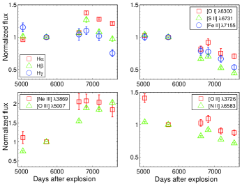
Figure 2: Upper panels: Fluxes for the unshocked, narrow component from the northern part of the ring, normalized to the flux at Oct. 2002 (day 5703). Lower panels: Fluxes for the southern part of the ring.

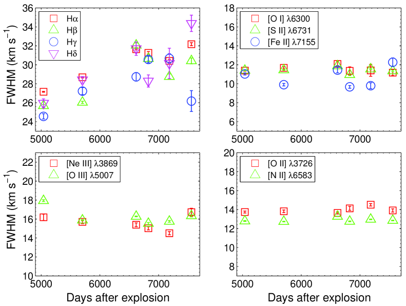
Figure 3: FWHM of the unshocked components as a function of time for the northern part of the ring.

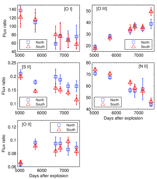
Figure 4: Diagnostic line ratios from the unshocked northern and southern components. The ratios shown are [O I] $(\lambda 6300+\lambda 6364)/\lambda 5577$, [O III] $(\lambda 4959+\lambda 5007)/\lambda 4363$, [S II] $(\lambda 4069+\lambda 4076)/(\lambda 6716+\lambda 6731)$, [O II] $(\lambda\lambda 7319-7331)/(\lambda 3726+\lambda 3729)$ and [N II] $(\lambda 6548+\lambda 6583)/\lambda 5755$.

3.3 Evolution of the shocked components

3.3.1 Line fluxes

The shocked gas is dominated by emission from the hot spots. A complete list of lines from the shocked component is given in Table 2 in G08. The fluxes of a selection of representative lines from the intermediate velocity component are shown in Fig. 5 and Fig. 6 for the northern and southern components, respectively. As with the narrow lines, we have normalized the fluxes, but in this case to Epoch 4 (2005 April) to facilitate a comparison of the different lines more directly. The absolute values of the fluxes can be found in Tables LABEL:tab:broadlines_n and LABEL:tab:broadlines_s in the Appendix. For comparison we also show the evolution of the integrated soft X-ray flux in the 0.5 – 2 keV range from Park et al. (2007).

As was already found in Gröningsson et al. (2006) for the high ionization lines, the line emission from the shocked gas increases rapidly as more ring gas is swept up by the shock. Here we confirm that this is a general feature for all lines. The rate of increase is, however, different for the different lines (Fig. 5). The low ionization lines of He I, [N II], [O I], [S II] and [Fe II] increase similar to each other and to the Balmer lines. This is also the case for the [Fe XIV] line. The intermediate ionization lines, [O III], [Ne III], [Ne V], [Fe III] and [Fe VII], however, all show a break between day $6500$ and day $7000$. This is probably also the case for the [Fe X] and [Fe XI] lines, although this result is close to the systematic uncertainties. The same pattern is seen for the southern component (Fig. 6). The Balmer decrement, as seen in H$\alpha$, H$\beta$, H$\gamma$, and H$\delta$, is constant within the systematic errors.

Figure 5: Fluxes for the shocked component from the northern part of the ring for selected lines, normalized to the flux at Apr. 2005 (day 6618). The lower right panel shows the soft X-ray flux normalized to the same date (from Park et al. 2007).

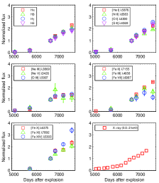
Figure 6: Same as Fig. 5, but for the southern part of the ring. Note the change of flux scale compared to Fig. 5.

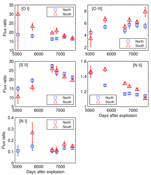
Figure 7: Diagnostic line ratios from the shocked northern and southern components. The ratios shown are [O I] $(\lambda 6300+\lambda 6364)/\lambda 5577$, [O III] $(\lambda 4959+\lambda 5007)/\lambda 4363$, [S II] $(\lambda 4069+\lambda 4076)/(\lambda 6716+\lambda 6731)$, [N I] $(\lambda 5198+\lambda 5200)/\lambda 3467$ and [N II] $(\lambda 6548+\lambda 6583)/\lambda 5755$. Note that the [O III] $\lambda 4363$ line profiles have been deblended from [Fe II] $\lambda 4358$ which makes the [O III] flux ratios somewhat more uncertain.

The flux ratios for the shocked components, plotted in Fig. 7, are useful diagnostics for the shocked gas, being sensitive to both electron density and temperature. In G08 we found that the densities are consistent with the compressions from radiative shocks. The electron density in the [O III] region was constrained to be in the range $\sim 10^{6}-10^{7}\mbox{ cm}^{-3}$ and with a temperature in the interval $\sim(1-4)\times 10^{4}\rm\leavevmode\nobreak\ K$ for both the northern and southern parts of the ring (see also Pun et al. 2002).

For [S II] we find a density of $n_{e}\ga 10^{7}\mbox{ cm}^{-3}$ and a temperature of the order of $T_{e}\sim 5000\rm\leavevmode\nobreak\ K$ in this region, while [O I] has a somewhat higher temperature, $T_{e}\sim 8000\rm\leavevmode\nobreak\ K$, and [N II] implies a marginally higher temperature than for [O I]. This result is confirmed by continued observations, but we also see some evolution in the line ratios in Fig. 7, consistent with an increasing temperature for [S II], [N II] and [O I].

The [O III] flux ratio $j_{\lambda\lambda 4959,5007}/j_{\lambda 4363}$ is temperature sensitive for the considered density interval. The data suggest that the emission comes from a region with an electron density of a few times $10^{6}\rm\leavevmode\nobreak\ cm^{-3}$ and a temperature around $15,000-20,000\rm\leavevmode\nobreak\ K$. It is difficult to find a clear trend for the evolution of the flux ratio, perhaps because the line [O III] $\leavevmode\nobreak\ \lambda 4363$ is blended with [Fe II]$\leavevmode\nobreak\ \lambda 4358$, and as a consequence has a relatively large uncertainty in flux.

3.3.2 Line profiles

Figure 8 illustrates the evolution of the H$\alpha$, [N II] $\leavevmode\nobreak\ \lambda 6583$, [O III] $\leavevmode\nobreak\ \lambda 5007$, and [Fe XIV] $\leavevmode\nobreak\ \lambda 5303$ line profiles from Epochs 2 to 7. These have been selected to represent a broad range of ionization stages, as well as a maximum S/N. We have subtracted the underlying broad emission of H$\alpha$ from the reverse shock to determine the profiles of the emission from the shocked gas for H$\alpha$ and [N II] $\leavevmode\nobreak\ \lambda 6583$, and for the other lines the continuum. Any blends have been subtracted using the procedure in G08. To facilitate a comparison between the different dates we have for this figure normalized the flux to the peak flux of the line profile.

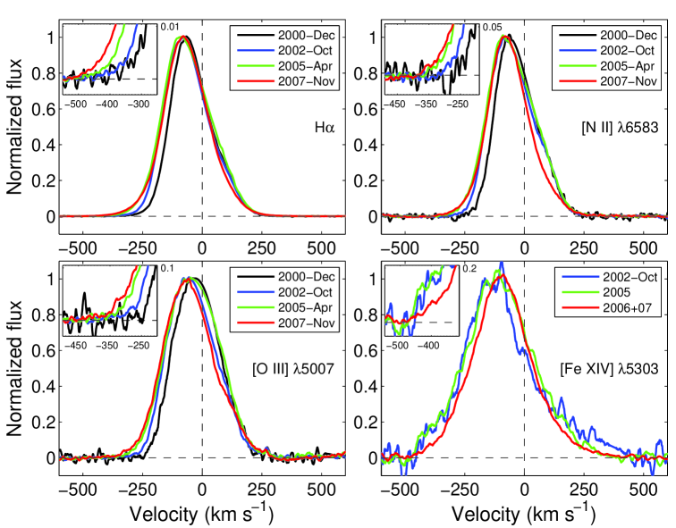
Figure 8: Evolution of the H$\alpha$, [N II] $\leavevmode\nobreak\ \lambda 6583$, [O III] $\leavevmode\nobreak\ \lambda 5007$, and [Fe XIV] $\leavevmode\nobreak\ \lambda 5303$ profiles from the shocked gas at the northern part of the ring. The insert in each panel show the blue wings of the lines to more clearly show the extent of the high velocity tail in each line. To increase the S/N for the [Fe XIV] $\leavevmode\nobreak\ \lambda 5303$ line we have added observations from 2006 – 2007. The zero velocity corresponds to the rest frame of the northern part of the ring.

Although the whole line profile evolves from epoch to epoch, the figures reveal that between Epochs 2 to 7 the largest increase in flux takes place for the blueshifted emission. In particular, the high velocity end of the blue wing shows a steady increase in velocity with time. In Fig. 9 we show the peak velocity and the velocity at a level of 5 % of the peak flux as a function of time for the different lines. The 5 % level has been chosen in order to facilitate a comparison between the low ionization lines, like H$\alpha$, with the high ionization coronal lines, like [Fe XIV] (in the same way as in G08). The latter has a considerably noisier profile due to the low flux (only $\!\!\!\phantom{\leq}\smash{\buildrel\over{\lower 2.67502pt\hbox{$\buildrel\lower 2.14001pt\hbox{$\displaystyle<$}\over{\sim}$}}}\,\,1$ % of H$\alpha$) and disappears in the noise at levels less than $\sim 5\%$ of the peak emission. We discuss the velocity at lower levels in Sect. 4.2.

The peak velocity in Fig. 9 only marginally evolves with time in both the southern and northern regions. There are, however, noticeable differences between the velocity values for the different lines. The low ionization lines, H$\alpha$, [O I] and [N II], have all similar velocities, while the [O III] and [Fe XIV] lines have lower and higher peak velocities, respectively, showing that contribution to the different lines probably come from different regions covered by the slit.

In addition, there are clear differences in peak velocities of the lines at the northern part of the ring compared to those in the southern part (Fig. 9). The velocities are considerably higher on the northern part which is likely due to a line-of-sight projection effect (see Sect. 4.2). In G08 we compared these peak velocities with the velocities obtained by the VLT/SINFONI instrument, which has an adaptive optics supported integral field spectrograph (Kjær et al. 2007). While the spatial resolution for SINFONI is much higher than for our UVES observations, the spectral resolution is low, $67-150\rm\leavevmode\nobreak\ km\leavevmode\nobreak\ s^{-1}$ in the different bands, and only gives an average, bulk velocity at each point on the ring. As found in G08, there is good agreement at the epoch of the first SINFONI observation in November 2004.

Turning now to the maximum velocity in Fig. 9 we see an interesting difference between the lines, as well as an evolution in time. While the low and intermediate ionization lines, H$\alpha$, [O I], [N II] and [O III], show similar velocities, $250-300\rm\leavevmode\nobreak\ km\leavevmode\nobreak\ s^{-1}$, the coronal lines have considerably higher velocities, $\sim 350\rm\leavevmode\nobreak\ km\leavevmode\nobreak\ s^{-1}$ for [Fe X] and $\sim 450\rm\leavevmode\nobreak\ km\leavevmode\nobreak\ s^{-1}$ for [Fe XIV]. Again, this shows that the two sets of lines come from regions of quite different physical conditions. We will discuss this in more detail in Sect. 4.2. There is an indication that the coronal line profiles, such as [Fe XI-XIV], become less blueshifted over time for the northern part of the ring. The maximum velocity (FWZI) does, however, not decrease with time, as seen in Fig. 8.

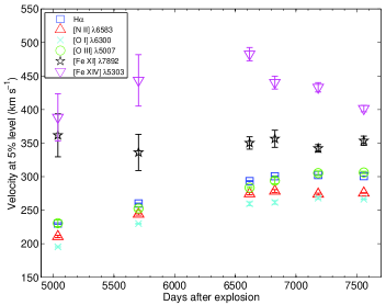
Figure 9: Upper panels: Velocities of the peak of the lines for the shocked component. Lower panel: Velocities at 5% flux level for the shocked component from the northern part of the ring.

4 Discussion

In this section we discuss the implications of the results in Sect. 3. The general picture we here have in mind for the optical emission is that of a radiative shock, moving into the dense ER, with a pre-shock density of $3\times 10^{3}-3\times 10^{4}\mbox{ cm}^{-3}$ and a temperature of $\sim(1-4)\times 10^{4}\rm\leavevmode\nobreak\ K$ (see below). The narrow line emission comes from this gas. The soft X-rays, as well as the coronal lines, then come from the immediate post-shock gas, with a temperature of $\sim(1-3)\times 10^{6}\rm\leavevmode\nobreak\ K$ and a density four times that of the pre-shock density. As the gas cools to $\sim 10^{4}\rm\leavevmode\nobreak\ K$, the density increases by a similar factor to $10^{6}-10^{7}\mbox{ cm}^{-3}$. This is where most of the optical, intermediate velocity lines arise. We now discuss these regions, one by one.

4.1 The narrow, unshocked lines

In connection with the shock breakout the rings were ionized by the soft X-rays during the first hour (Lundqvist & Fransson 1996). After this they have recombined and cooled at a rate determined mainly by the density of the different parts of the rings. However, because of the strong X-ray flux from the shocks propagating into the dense blobs one expects re-heating and re-ionization of this gas, as well as gas in the inner ring and surrounding gas that was never ionized by the supernova flash. The decrease in the line fluxes after the flash ionization is therefore expected to turn into an increase, or at least a slower decay, when preionization by the shocks starts to dominate the conditions in the ring. The evolution of the narrow components of the different lines is therefore of great interest.

As shown in Fig. 2, we do indeed find that the evolution of the fluxes of the narrow lines is different for different lines. The [O I], [O II], [N II], [S II] and [Fe II] lines all decrease with time (Fig. 2). These lines are all collisionally excited and therefore sensitive to both temperature and degree of ionization. The hydrogen lines arise mainly by recombination and therefore decay slower than the collisionally excited lines, as is observed.

The most interesting result is, however, the observed increase of the [O III] and [Ne III] lines up to day $\sim 6800$. After this epoch the fluxes of these lines become constant or decrease. This behavior is consistent with calculations of the shock structure of a radiative shock. Soft X-rays from the shock ionize and heat the pre-shock gas to a temperature of $(2-3)\times 10^{4}$ K immediately in front of the shock (Allen et al. 2008). The absorbed X-rays are there re-emitted as UV and optical lines. The interesting point is now that these shock calculations show that the [O III] $\leavevmode\nobreak\ \lambda\lambda 4959,5007$ lines are by far the strongest optical lines from this region. The fact that these lines show an increase in the fluxes is therefore consistent with the shock models, and strongly indicates that the radiation from the shock interaction started to affect the unshocked ring already several years ago.

The levelling off of the [O III] and [Ne III] lines between day $6500$ and day $7000$ may be a result of several factors. One possibility is that all the gas in the ring with high enough density to be visible (i.e., $n_{e}\!\!\!\phantom{\geq}\smash{\buildrel\over{\lower 2.67502pt\hbox{$\buildrel\lower 2.14001pt\hbox{$\displaystyle>$}\over{\sim}$}}}\,\,10^{3}\rm\leavevmode\nobreak\ cm^{-3}$) has been ionized by the X-rays, which will result in a nearly constant flux after this epoch. It could, of course, also be the result of a decreasing X-ray flux from the shocks, or finally from sweeping-up of the dense gas by the shocks.

Similarly, the fast decrease of the low ionization lines may either be a result of ionization or sweeping-up of the unshocked gas. Future HST imaging may distinguish between these scenarios.

A more detailed picture of the physical conditions of the narrow-line emitting gas can be obtained from line ratios (see Fig. 4). The declining diagnostic ratios of [N II], [O I] and [S II] all suggest an increasing temperature in this zone, which may be indicative of pre-ionization.

For the [O II] and [O III] lines we see a rather dramatic change between Epochs 2 and 3 compared to at later epochs. The low ratios for [O III] $j_{\lambda\lambda 4959,5007}/j_{\lambda 4363}$ at Epoch 2 indicate much higher temperatures in both the northern and southern parts of the ring than at later epochs. Using nebular analysis as in G08, the [O III] temperature appears to decline from $\sim 5\times 10^{4}$ K to $\sim 2.5\times 10^{4}$ K between Epoch 2 and 3, and further down to $\sim 2\times 10^{4}$ K at later epochs. The Epoch 2 temperature is clearly much higher than expected from a shock precursor (cf. above, see also Allen et al. 2008).

The most likely reason for this is that the narrow-line emission at the earliest epochs comes mainly from low-density gas that was flash-ionized by the supernova. Mattila et al. (2003, and paper in preparation) show that the density of the flash-ionized gas dominating the [O III] emission at epochs around 5000 days is $\sim 1\times 10^{3}\mbox{ cm}^{-3}$. The [O III] temperature in these models is $\sim 5\times 10^{4}$ K, i.e., close to what we observe. From an inspection of the HST images (see Fig. 1) it is also clear that by day $\sim 5000$ rather few spots on the ring have been shocked, and that most of the emission within the UVES slit at Epoch 2 comes from the diffuse, rather evenly distributed, emission between the blobs. This is even more pronounced in [O III] than the H$\alpha$+[N II] emission shown in Fig. 1. Note also that only a fraction of the emission from the blobs seen in the HST images stems from narrow-line emitting shock precursors, as the HST images cannot distinguish between that emission and the line emission from the shocked gas.

At Epoch 2, we estimate that $\!\!\!\phantom{\leq}\smash{\buildrel\over{\lower 2.67502pt\hbox{$\buildrel\lower 2.14001pt\hbox{$\displaystyle<$}\over{\sim}$}}}\,\,30$% of the narrow-line [O III] $\lambda\lambda 4959,5007$ emission comes from shock precursors, and that the rest comes from the diffuse low-density gas. For [O III] $\lambda 4363$ the fraction would then be $\!\!\!\phantom{\leq}\smash{\buildrel\over{\lower 2.67502pt\hbox{$\buildrel\lower 2.14001pt\hbox{$\displaystyle<$}\over{\sim}$}}}\,\,15$% to obtain the observed $j_{\lambda\lambda 4959,5007}/j_{\lambda 4363}$ ratio. However, already by Epoch 3, the narrow [O III] $\lambda\lambda 4959,5007$ emission within the UVES slit should be dominated by shock precursors, whereas the narrow [O III] $\lambda 4363$ would still be “contaminated” and perhaps even dominated by the $\sim 1\times 10^{3}\mbox{ cm}^{-3}$ component which would then still have a temperature of $\sim(4-5)\times 10^{4}$ K, according to the models discussed in Mattila et al. (2003). The higher temperature for [O III] $\lambda 4363$ is directly supported by the larger line width for that line seen at Epoch 3, compared to the other two [O III] lines (G08).

This two component model is also consistent with the evolution of the fluxes from the narrow and intermediate velocity components. The increase in the flux of the intermediate-velocity component of [O III] $\lambda\lambda 4959,5007$ should correlate with the narrow-line flux from the precursor. Between Epochs 2 and 3, the former increases by a factor $\sim 3.4$ for the northern part of the ring, while the narrow velocity component only increases by a factor of $\sim 1.3$. However, after Epoch 3, when the precursor emission is likely to dominate [O III], the increase of the narrow component is similar to the intermediate velocity flux.

The extent of the pre-ionized zone depends on the number of ionizing photons from the cooling shock, which should scale as the total flux ${1\over 2}\rho V_{s}^{3}$. The number of recombinations per unit area is $\alpha_{B}n_{e}^{2}\Delta x({\rm HII})$, where $\Delta x({\rm HII})$ is the thickness of the ionized region and $\alpha_{B}$ is the Case B recombination rate. Therefore, $\Delta x({\rm HII})\propto V_{s}^{3}/\alpha_{B}n_{e}^{2}$. This describes well the shock calculations by Allen et al. (2008), which gives the normalization, and we find

$$\Delta x({\rm HII})\approx 1.4\times 10^{16}\left({V_{s}\over 200\rm\leavevmode\nobreak\ km\leavevmode\nobreak\ s^{-1}}\right)^{3}\left({n_{e}\over 10^{4}\mbox{ cm}^{-3}}\right)^{-1}{\rm\leavevmode\nobreak\ cm.}$$ (2)

The pre-ionized region is therefore sensitive to both the shock velocity, which probably spans a range $100-400\rm\leavevmode\nobreak\ km\leavevmode\nobreak\ s^{-1}$, as well as the density. It is clear that a large fraction of the ring may be pre-ionized by the shocks, as well as material outside of the ER, which is likely to have a lower density.

4.2 Shocked intermediate component

From Fig. 5 and Fig. 6 we found that the lines from the shocked gas increase by a factor of $\sim 4$ from day 5703 to around day 7000 for the northern ring, and by an even larger factor for the southern ring. This is similar to that of the soft X-rays, and for comparison we show the evolution of the soft X-rays from Park et al. (2007) as the lower right panels in Fig. 5 and Fig. 6. Note that the X-ray flux is that of the total ring flux, while our fluxes represent two different regions. We find nevertheless that the optical flux and soft X-ray flux have a very similar evolution, and that they therefore are likely to come from the same region.

One of the most important results in our study of the shocked, intermediate velocity component is the increase in the widths (FWZI) of the low ionization lines (Fig. 8). With the exception of the coronal lines, the optical line emission must originate in radiative shocks. The widths of the shocked emission lines are therefore expected to increase with time as faster shocks become radiative. However, the line profiles only reflect the projected shock velocities along the line of sight, and consequently, the FWZI velocity is only a lower limit to the maximum velocities of the radiative shocks driven into the protrusions. Nevertheless, if conditions are similar, a steady increase in the line widths with time is therefore a strong indication that gas from shocks with increasingly higher shock velocity did have time to cool. This is further strengthened by the fact that in G08 we found that the line widths of the low ionization lines in 2002 were considerably smaller than those of the coronal lines. Now, in our last observations in 2007 (Epoch 7) the maximum blueward velocities of the low ionization lines are approaching those of the coronal lines (Fig. 9).

The maximum velocities estimated in Fig. 9 are based on the velocity at 5 % of the peak flux. This was mainly motivated by the requirement to compare the coronal lines with the low ionization lines. Because of the high S/N of the strong lines we can detect the line wings to considerably lower levels to get a better estimate of the true velocity extent of the lines. In Fig. 10 we show the maximum velocity from the northern and southern parts of the ring for H$\alpha$, [N II], [O I] and [O III], now at a 1 % level of the peak flux. We here see the same increase in maximum velocity with time as in Fig. 9, although the velocities are considerably higher. From Fig. 8 we see that H$\alpha$ can in fact be traced to $\sim 500\rm\leavevmode\nobreak\ km\leavevmode\nobreak\ s^{-1}$ in the last spectrum. The same is true for the southern part of the ring.

As can be seen from Figs. 9 and 10, the velocities from the southern part of the ring are consistently lower by $\sim 40\rm\leavevmode\nobreak\ km\leavevmode\nobreak\ s^{-1}$, but do also show a similar increase with time as those from the northern part. The lower velocities may either be a projection effect, an effect of the later impact in this region, or a higher density. Even though there is clearly a time delay between the northern and southern parts of the ring ($\sim 300$ days), the most plausible explanation is a difference in the projection of velocities between the two regions. The flux from the northern part mainly comes from “hot spots” between $\sim 0^{\circ}-50^{\circ}$ while spots between $\sim 230^{\circ}-250^{\circ}$ dominate the flux from the southern part (see Fig. 1). This asymmetric distribution of “hot spots” between the northern and southern parts of the ring could well account for a difference in projection such that the line-of-sight velocities from the southern part are consistently lower than the velocities from the northern part, consistent with the observed line profiles. This is also supported by the similar difference in peak velocity, which is $40-50\rm\leavevmode\nobreak\ km\leavevmode\nobreak\ s^{-1}$ (see also Kjær et al. 2007).

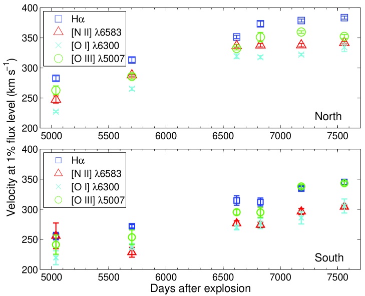
Figure 10: Velocities at 1% flux level for the shocked gas from the northern and southern components.

For a shock to become radiative it must cool from its postshock temperature to $\sim 10^{4}$ K from the time it was shocked. From shock calculations we found that the time it takes for a shock to become radiative, i.e., the cooling time, $t_{\rm cool}$, is related to the preshock density and the shock velocity as

$$t_{\mathrm{cool}}\approx 8.3\left({n_{\mathrm{spot}}\over 10^{4}\mbox{ cm}^{-3}}\right)^{-1}\left({V_{s}\over 300\rm\leavevmode\nobreak\ km\leavevmode\nobreak\ s^{-1}}\right)^{3.4}\ \rm years$$ (3)

(Gröningsson et al. 2006), where $n_{\mathrm{spot}}$ is the pre-shock density of the ring.

At Epoch 3 (October 2002) the shocks had $\sim 7\rm{\leavevmode\nobreak\ years}$ to cool since first impact (taken as $1995$; see Lawrence et al. 2000), and from the FWZI of the line profiles, we estimate that shocks with velocities $\!\!\!\phantom{\leq}\smash{\buildrel\over{\lower 2.67502pt\hbox{$\buildrel\lower 2.14001pt\hbox{$\displaystyle<$}\over{\sim}$}}}\,\,300\rm\leavevmode\nobreak\ km\leavevmode\nobreak\ s^{-1}$ have had enough time to cool. This places a lower limit on the preshock density from Eq. (3) and we estimate $n_{\mathrm{spot}}\!\!\!\phantom{\geq}\smash{\buildrel\over{\lower 2.67502pt\hbox{$\buildrel\lower 2.14001pt\hbox{$\displaystyle>$}\over{\sim}$}}}\,\,1.2\times 10^{4}\mbox{ cm}^{-3}$. At our last epoch the maximum velocity of H$\alpha$ is $\sim 500\rm\leavevmode\nobreak\ km\leavevmode\nobreak\ s^{-1}$. With this velocity Eq. (3) implies a density of $n_{\mathrm{spot}}\!\!\!\phantom{\geq}\smash{\buildrel\over{\lower 2.67502pt\hbox{$\buildrel\lower 2.14001pt\hbox{$\displaystyle>$}\over{\sim}$}}}\,\,2.7\times 10^{4}\mbox{ cm}^{-3}$.

These densities can be compared to the densities derived from the analysis of the ring during the first few years after outbreak. Lundqvist & Fransson (1996) find that the light curves of the ring emission require a range in densities from $6\times 10^{3}\mbox{ cm}^{-3}$ to $3.3\times 10^{4}\mbox{ cm}^{-3}$. Further, Mattila et al. (2003, and paper in preparation) show that later observations of the narrow optical lines require densities down to $\sim 10^{3}\mbox{ cm}^{-3}$. This density agrees with the limit on the ionization time $n_{e}t_{i}\!\!\!\phantom{\geq}\smash{\buildrel\over{\lower 2.67502pt\hbox{$\buildrel\lower 2.14001pt\hbox{$\displaystyle>$}\over{\sim}$}}}\,\,10^{12}\mbox{ cm}^{-3}{\rm\leavevmode\nobreak\ s}$ found from the soft X–rays by Park et al. (2007). Using this, and the assumed impact times between $4000-6000$ days after the explosion, Dwek et al. (2008) find a range of $(0.3-1.4)\times 10^{3}\mbox{ cm}^{-3}$, which should be seen as a lower limit to the density of the pre-shock gas. It is likely that we now see the densest blobs cooling down first, and the agreement with the densities determined for the ring before the collision makes this scenario likely. As time goes, gas shocked by higher velocity shocks and/or lower densities will gradually cool down.

In G08 we showed that the line width of the low ionization lines were considerably smaller than the coronal lines in 2002 (see also Fig. 9). A likely interpretation is that part, or all, of the gas emitting the coronal lines at that time had not yet had time to cool and be seen as optical low ionization emission lines. The fact that the H$\alpha$ velocities from the northern part are now comparable to those of the coronal lines is consistent with the estimates of the cooling time above. In Fig. 5 we see that all lines increased in flux up to day $\sim 6800$. After this epoch there are, however, clear differences between the various lines. While low ionization lines, such as [O I], [N II], [S II] and [Fe II] continue to increase, the intermediate ionization lines of [O III] and [Ne III] show a break, and are consistent with being either constant or even decreasing in flux.

The evolution of the [O II] and [O III] line fluxes may be understood as a result of radiative shocks, which have not yet had time to cool completely. In such a shock, gas with a given ionization stage will first increase its emission measure as gas is recombining. After some time this gas will recombine to the next lower ionization stage and an equilibrium will be set up, where the emission measure of the ion will be constant. This will continue to lower and lower ionization stages. At the lowest ionization stage, this will, however stop and its emission measure will instead continously increase as long as more cooling gas is accumulating and the cooling time at this temperature is long compared to the age. Applied to oxygen, this means that [O I], [O II] and [O III] will all initially increase. After some time, [O II] and [O III] will reach a steady state, while [O I] will continue to increase, just as observed. The same applies to sulphur and iron, although it will in these cases stop at [Fe II] and [S II], because of photoionization of Fe I and S I. The lower ionization lines will therefore continue to increase as long as new gas is shocked and the cooling time is long compared to the age of the shock. This picture has been confirmed with numerical calculations.

[Fe XIV] and other coronal lines are special in that they may come from both radiative and adiabatic shocks, as long as the temperature behind the shock is $\!\!\!\phantom{\leq}\smash{\buildrel\over{\lower 2.67502pt\hbox{$\buildrel\lower 2.14001pt\hbox{$\displaystyle<$}\over{\sim}$}}}\,\,5\times 10^{6}\rm\leavevmode\nobreak\ K$. At least part of their emission may therefore be from non-radiative shocks, which is consistent with the more extended line profiles, especially at early epochs.

In a recent paper Dewey et al. (2008) find that (adiabatic) shock model fits of the X-ray line fluxes indicate a bimodial distribution of temperature. The dominant component has a temperature of $\sim 0.55$ keV, nearly constant between 2004 and 2007. The hard component, on the other hand, decreases from $\sim 2.7$ keV in 2004 to $\sim 1.9$ keV in 2007. Although uncertain, the FWHM of the lines correspond to a shock velocity of $200-450\rm\leavevmode\nobreak\ km\leavevmode\nobreak\ s^{-1}$. This is comparable to our optical velocities and strengthens the identification of the soft X-ray component with the optical lines, as was already indicated from the flux evolution. The harder X-ray component does, however, not have any corresponding optical component. Further, a temperature of $\sim 2.3$ keV corresponds to a shock velocity of $\sim 1400\rm\leavevmode\nobreak\ km\leavevmode\nobreak\ s^{-1}$. Such a component should be adiabatic for a very long time. From the fact that such a high velocity is not seen in the line widths, Dewey et al. suggest that the high velocity component may originate from a reflected shock, moving back into the previously shocked gas.

An interesting additional fact is that the Chandra imaging shows an expansion of the X-ray emitting plasma corresponding to a velocity of $1400-1500\rm\leavevmode\nobreak\ km\leavevmode\nobreak\ s^{-1}$ (e.g., Park et al. 2007). Also the extent of the optical emission increases with a similar velocity (P. Challis priv.comm.). In $\sim 10$ years the emitting region has therefore expanded by $\sim 3\times 10^{16}{\rm\leavevmode\nobreak\ cm}$, which is a considerable fraction of the thickness of the visible ring. As Dewey et al. (2008) point out, this expansion is, however, likely to take place in a low density component, and not in the dense clumps. We expect this expansion to continue as long as there is low density gas in the vicinity of the clumps.

5 Summary

We have presented high spectral resolution UVES observations at multiple epochs of the inner circumstellar ring of SN 1987A. Due to the high spectral resolution, we are able to separate the shocked from the unshocked ring emission, as well as to study the evolution of the fluxes and line profiles of the different lines.

For the narrow lines we find strong evidence for pre-ionization of the unshocked ring by the soft X-rays from cooling gas behind the shocks. This is indicated both by the increasing [O III] flux and from the temperature inferred from the low ionization lines [N II], [O I] and [S II]. The increasing [O III] line ratios at the early epochs (until day $\sim 5700$) are consistent with emission coming mainly from very low density regions ($\sim 1\times 10^{3}\rm\leavevmode\nobreak\ cm^{-3}$) ionized by the SN flash in connection with the explosion. Later on, however, the emission is dominated by gas pre-ionized by the X-rays.

For the intermediate velocity low ionization lines, we find evidence for increasing line widths for the shocked components. This is to be expected as faster shocks will have enough time to become radiative and cool. At the latest epoch the H$\alpha$ line profile extends to $\sim 500\rm\leavevmode\nobreak\ km\leavevmode\nobreak\ s^{-1}$ for both the northern and southern part of the ring, which is comparable to the maximum velocity of the coronal lines. The ring collision in SN 1987A is therefore one of the best examples of high velocity radiative shocks we have. Together with the X-ray observations these observations therefore offer a unique opportunity to study this class of shocks in detail.

The difference in shapes for the line profiles between the northern and southern components cannot solely be explained by a time delay effect, but is most likely explained by a difference of projection of the shock velocities caused by the locations of “hot spots” around the ring.

We find a correlation of our optical light curves to that of the soft X-rays. This suggests that most of the optical lines and soft X-rays arise from the same region. The difference in line widths of the coronal lines and the low ionization lines at early epochs indicates that at least some of the coronal emission comes from adiabatic shocks. Short of day $\sim 7000$ we find that the optical light curves of the intermediate ionization lines such as [O III] and [Ne III] is levelling off and especially so on the northern part of the ring. We argue that this is due to the fact that with time the gas will recombine to lower ionization stages until the lowest stage is reached. If, however, the fluxes from the optical lines have started to decline, just as the narrow optical lines have done, this may be an indication that the forward shocks have now started to interact with gas with lower densities. Future observations will shed more light on this.

Appendix A Comparison of fluxes from HST and UVES.

Pipeline-processed HST imaging have been obtained by the SAINTS team (PI: R.P. Kirshner) at similar epochs as for the UVES spectra. The instruments were WFPC2 with narrow-band filters F502N and F656N at day 5013 and ACS with filters F502N and F658N (at days 5795-7229).

In order to compare the HST fluxes with the fluxes of UVES we first converted the counts per electrons in the HST images to flux density units (given in$\rm\leavevmode\nobreak\ erg\leavevmode\nobreak\ s^{-1}cm^{-2}\AA^{-1}$). Thus, the images were multiplied by the PHOTFLAM header keyword and, in the case of WFPC2 images, also divided by the exposure time. The next step was to rotate the images to $30^{\circ}$ in accordance with the slit rotation for the UVES spectra. To account for the moderate seeing of the ground-based UVES exposures (typically $\sim 0\aas@@fstack{\prime\prime}8$) we artificially added this seeing to the HST images by convolving each image with a two-dimensional Gaussian kernel.

All the pixel columns in the images within $0\aas@@fstack{\prime\prime}4$ from the center of the SN (the aperture corresponding to the width and location of the UVES slit) were summed. In this way we obtained spatial flux profiles which correspond to that of the UVES spectra. The LMC background emission level was estimated by fitting a second-order polynomial to the regions outside the outer rings. The polynomial was then subtracted from the total spatial profile.

The HST fluxes could now be extracted in similar way to the UVES spectra by fitting a two-Gaussian profile to the bimodal spatial ring profiles. The area under each Gaussian then corresponds to the northern and southern part of the ring respectively (see G08 for more details).

To compare the fluxes obtained from the HST images with the UVES fluxes, we performed a bandpass spectrophotometry of the spectra. Hence, we obtained the HST filter transmission functions by using the IRAF task calcband in the hst/synphot package and then integrated the UVES fluxes over the normalized versions of these.

The UVES bandpass fluxes have been plotted for different epochs and are compared with WFPC2 filter F656N and ACS filter F658N images (Fig. 11). In the same way, the UVES bandpass fluxes are compared with the WFPC2 and ACS filters F502N in Fig. 12.

In Fig. 11 we see that we can directly compare the UVES bandpass fluxes at day 5039 with that obtained by HST/WFPC2 at day 5013. We find that the UVES flux is $87\%$ of the corresponding HST flux on the northern part of the ring and $82\%$ on southern part. For the ACS fluxes, the largest deviation occur at Epoch 4 (day 6618). At this epoch the UVES fluxes on the northern and southern parts of the ring are $90\%$ of that obtained from HST/ACS at day 6613.

We now turn to Fig. 12 for the F502N filter. A comparison between the UVES fluxes at day 5039 with the HST/WFPC2 fluxes at day 5013 reveals that the UVES flux is $83\%$ of that of HST on the northern part and $90\%$ on the southern part of the ring. For the ACS we find that the deviations between the HST fluxes and the corresponding UVES fluxes are within $\sim 15\%$.

From this analysis we estimate that the uncertainty in the UVES absolute fluxing should be less than $\sim 20\%$. In addition, comparing the fluxes from filter F656N/F658N with those from filter F502N give us a clue about the accuracy of the relative fluxes between different parts of the spectra and we find that the uncertainty should be less than $\sim 10\%$. The UVES spectrograph is equipped with three different CCDs (see Sect. 2), one in the blue part of the spectrum ($\sim 303-499\leavevmode\nobreak\ \rm{nm}$) and two in the red part ($\sim 476-577\leavevmode\nobreak\ \rm{nm}$ and $\sim 583-684\leavevmode\nobreak\ \rm{nm}$ respectively for the standard setting 346+580). Hence, in this analysis we are only probing the fluxes for two out of the three CCDs and the uncertainty in the relative fluxes can therefore possibly be larger for emission lines situated in the blue part of the spectrum. The relative fluxes over the whole spectral range have, however, been checked against UVES spectrophotometric standard star spectra (see Sect. 2).

Moreover, to check the robustness of these results we varied the artificially imposed seeing on the HST images between $0\aas@@fstack{\prime\prime}4$ and $1\aas@@fstack{\prime\prime}0$. This showed that the total flux covered by the slit is fairly insensitive for this seeing range, and differs by less than a few percent. The redistribution effect of the fluxes from different parts of the ring is, of course, still important as the seeing is varied. The net effect here is that the flux on the northern part of the ring tends to decrease with increasing seeing, while the opposite effect holds for the southern part. This is explained by the fact that the “hot spots” are distributed unevenly around the ring (see Fig. 1) and this effect will therefore vary with time. We find that for some epochs, the individual fluxes from north and south respectively could shift by an amount of $\sim 10\%$ due to this effect.

In addition, from the HST images we can estimate the relation between the ring flux encapsulated by the slit and the total flux from the ring. For a simulated seeing of $0\aas@@fstack{\prime\prime}7$ we found that the factor between total ring flux and the flux encapsulated by the $0\aas@@fstack{\prime\prime}8$ wide slit was $2.4$ with an accuracy of $10\%$ for all epochs.

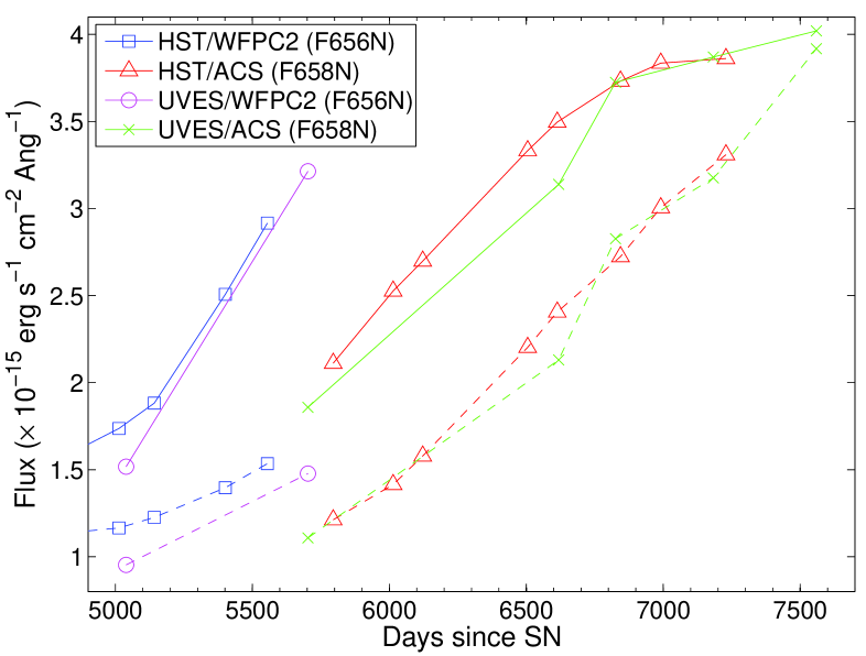
Figure 11: HST narrow-band filter fluxes for WFPC2 and ACS together with the corresponding UVES bandpass fluxes for the F656N and F658N filters for the northern part (solid lines) and the southern part (dashed lines) of the ring.

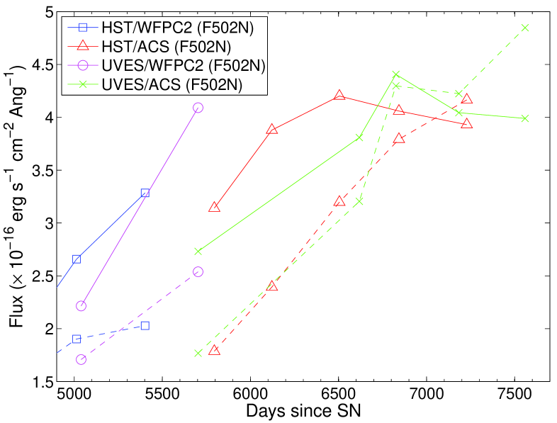
Figure 12: The same as Fig. 11 but for WFPC2 and ACS narrow-band filters F502N.

Appendix B Line fluxes

Table 2: Emission lines from the unshocked gas of the ER at Epoch 2.

			North			South
	Rest wavel.		$V_{\rm peak}^{\mathrm{c}}$	$V_{\rm FWHM}$		$V_{\rm peak}$	$V_{\rm FWHM}$	Extinction
Emission	Å	Relative fluxa	$\rm\leavevmode\nobreak\ km\leavevmode\nobreak\ s^{-1}$	$\rm\leavevmode\nobreak\ km\leavevmode\nobreak\ s^{-1}$	Relative fluxa	$\rm\leavevmode\nobreak\ km\leavevmode\nobreak\ s^{-1}$	$\rm\leavevmode\nobreak\ km\leavevmode\nobreak\ s^{-1}$	correctionb
[Ne V]	3425.86	$19.8\pm 2.7$	$282.1\pm 1.2$	$20.72\pm 0.72$	$17.2\pm 2.6$	$294.9\pm 1.3$	$18.59\pm 1.31$	2.06
[O II]	3726.03	$162.0\pm 4.7$	$283.1\pm 0.4$	$13.74\pm 0.10$	$152.4\pm 5.2$	$293.2\pm 0.4$	$14.30\pm 0.16$	1.98
[O II]	3728.82	$97.5\pm 5.8$	$280.6\pm 0.5$	$12.90\pm 0.22$	$101.4\pm 6.2$	$290.1\pm 0.5$	$15.06\pm 0.17$	1.98
[Ne III]	3868.75	$39.5\pm 2.6$	$281.7\pm 0.6$	$16.19\pm 0.34$	$29.6\pm 3.6$	$293.5\pm 0.9$	$17.75\pm 0.58$	1.94
[S II]	4068.60	$23.4\pm 1.5$	$281.4\pm 0.5$	$11.55\pm 0.19$	$22.3\pm 1.2$	$292.2\pm 0.5$	$12.95\pm 0.29$	1.90
[S II]	4076.35	$7.2\pm 1.5$	$281.9\pm 0.7$	$10.50\pm 0.55$	$8.3\pm 1.1$	$292.1\pm 0.7$	$12.56\pm 0.59$	1.90
H$\delta$	4101.73	$26.5\pm 2.1$	$281.4\pm 1.0$	$25.95\pm 0.45$	$26.1\pm 2.3$	$291.0\pm 1.0$	$26.91\pm 0.48$	1.89
H$\gamma$	4340.46	$48.4\pm 1.9$	$281.2\pm 0.8$	$24.56\pm 0.28$	$48.2\pm 2.2$	$291.3\pm 0.8$	$26.69\pm 0.25$	1.84
[O III]	4363.21	$11.2\pm 1.2$	$280.0\pm 1.1$	$21.19\pm 0.71$	$8.6\pm 1.2$	$292.8\pm 1.2$	$20.20\pm 1.19$	1.84
He II	4685.7	-	-	-	-	-	-	1.75
H$\beta$	4861.32	$100.0$	$282.0\pm 0.5$	$25.68\pm 0.12$	$105.9\pm 2.1$	$290.9\pm 0.4$	$26.69\pm 0.07$	1.71
[O III]	4958.91	$58.5\pm 1.9$	$281.7\pm 0.5$	$17.82\pm 0.17$	$41.0\pm 1.3$	$294.4\pm 0.6$	$21.92\pm 0.25$	1.68
[O III]	5006.84	$176.1\pm 4.6$	$281.7\pm 0.4$	$17.94\pm 0.09$	$124.7\pm 3.5$	$294.8\pm 0.5$	$21.95\pm 0.12$	1.67
[O I]	5577.34	$0.5\pm 0.2$	$282.2\pm 1.3$	$13.29\pm 1.17$	$0.5\pm 0.2$	$289.4\pm 1.6$	$17.75\pm 1.38$	1.57
[N II]	5754.59	$21.3\pm 0.6$	$282.0\pm 0.3$	$13.84\pm 0.08$	$20.5\pm 0.6$	$292.4\pm 0.4$	$14.87\pm 0.16$	1.54
He I	5875.63	$20.6\pm 0.8$	$281.2\pm 0.5$	$16.51\pm 0.14$	$19.3\pm 0.8$	$290.7\pm 0.5$	$17.77\pm 0.18$	1.53
[O I]	6300.30	$52.2\pm 1.4$	$281.5\pm 0.3$	$11.39\pm 0.07$	$52.3\pm 1.1$	$291.9\pm 0.3$	$13.20\pm 0.08$	1.47
[S III]	6312.06	$1.7\pm 0.3$	$281.2\pm 1.2$	$14.96\pm 1.13$	$1.1\pm 0.3$	$293.4\pm 1.5$	$17.47\pm 1.59$	1.47
[O I]	6363.78	$18.0\pm 0.5$	$281.3\pm 0.3$	$11.29\pm 0.05$	$18.5\pm 0.5$	$292.2\pm 0.3$	$13.69\pm 0.09$	1.47
[N II]	6548.05	$394.7\pm 8.6$	$282.3\pm 0.2$	$12.84\pm 0.04$	$397.5\pm 7.3$	$292.7\pm 0.2$	$14.18\pm 0.04$	1.45
H$\alpha$	6562.80	$395.1\pm 6.5$	$281.7\pm 0.3$	$27.15\pm 0.04$	$380.7\pm 6.2$	$290.8\pm 0.3$	$26.74\pm 0.04$	1.45
[N II]	6583.45	$1206.3\pm 24.2$	$280.8\pm 0.2$	$12.79\pm 0.04$	$1216.9\pm 20.2$	$291.5\pm 0.2$	$14.18\pm 0.03$	1.45
He I	6678.15	$5.7\pm 0.4$	$282.0\pm 0.6$	$15.91\pm 0.24$	$5.6\pm 0.3$	$292.1\pm 0.7$	$17.98\pm 0.44$	1.44
[S II]	6716.44	$72.8\pm 2.1$	$281.9\pm 0.3$	$11.82\pm 0.07$	$76.2\pm 1.9$	$292.9\pm 0.3$	$13.24\pm 0.06$	1.43
[S II]	6730.82	$121.1\pm 2.9$	$281.9\pm 0.3$	$11.40\pm 0.05$	$128.3\pm 2.7$	$292.8\pm 0.2$	$13.02\pm 0.05$	1.43
[Ar III]	7135.79	$6.1\pm 0.4$	$280.3\pm 0.5$	$14.86\pm 0.26$	$4.6\pm 0.4$	$292.2\pm 0.7$	$16.39\pm 0.62$	1.39
[Fe II]	7155.16	$5.1\pm 0.2$	$281.7\pm 0.4$	$11.03\pm 0.11$	$5.3\pm 0.2$	$293.8\pm 0.3$	$10.63\pm 0.23$	1.39
[O II]	7319d	$13.2\pm 0.8$	-	-	$13.2\pm 0.9$	-	-	1.37
[Ca II]	7323.89	$11.5\pm 0.4$	$280.6\pm 0.3$	$10.82\pm 0.08$	$11.2\pm 0.5$	$292.3\pm 0.4$	$11.06\pm 0.15$	1.37
[O II]	7330e	$10.7\pm 0.7$	-	-	$11.1\pm 0.7$	-	-	1.37
[S III]	9068.6	$14.0\pm 0.9$	-	$10.65\pm 0.24$	$8.4\pm 0.4$	-	$15.03\pm 0.25$	1.24
[S III]	9530.6+31.1	$30.7\pm 1.6$	-	$14.60\pm 0.24$	$18.1\pm 0.8$	-	$17.58\pm 0.22$	1.22

• Fluxes are relative to H$\beta$: “100” corresponds to $(29.3\pm 0.5)\times 10^{-16}\rm\leavevmode\nobreak\ erg\leavevmode\nobreak\ s^{-1}cm^{-2}$.

• $E(B-V)=0.16$, with $E(B-V)=0.10$ for LMC and $E(B-V)=0.06$ for the Milky Way.

• The recession velocity of the peak flux.

• Applies to both lines at $7318.92\mbox{ \AA}$ and $7319.99\mbox{ \AA}$.

• Applies to both lines at $7329.67\mbox{ \AA}$ and $7330.73\mbox{ \AA}$.

Table 3: Emission lines from the unshocked gas of the ER at Epoch 3.

			North			South
	Rest wavel.		$V_{\rm peak}^{\mathrm{c}}$	$V_{\rm FWHM}$		$V_{\rm peak}$	$V_{\rm FWHM}$	Extinction
Emission	Å	Relative fluxa	$\rm\leavevmode\nobreak\ km\leavevmode\nobreak\ s^{-1}$	$\rm\leavevmode\nobreak\ km\leavevmode\nobreak\ s^{-1}$	Relative fluxa	$\rm\leavevmode\nobreak\ km\leavevmode\nobreak\ s^{-1}$	$\rm\leavevmode\nobreak\ km\leavevmode\nobreak\ s^{-1}$	correctionb
[Ne V]	3425.86	$17.2\pm 1.7$	$281.7\pm 1.2$	$23.45\pm 0.58$	$13.8\pm 1.6$	$294.4\pm 1.0$	$19.55\pm 0.57$	2.06
[O II]	3726.03	$109.2\pm 4.1$	$283.0\pm 0.4$	$13.82\pm 0.13$	$101.1\pm 4.0$	$293.3\pm 0.5$	$14.77\pm 0.23$	1.98
[O II]	3728.82	$66.4\pm 3.7$	$280.1\pm 0.5$	$14.19\pm 0.20$	$63.8\pm 3.9$	$290.6\pm 0.6$	$14.87\pm 0.37$	1.98
[Ne III]	3868.75	$44.0\pm 1.8$	$281.3\pm 0.5$	$15.72\pm 0.18$	$24.7\pm 1.8$	$292.1\pm 0.7$	$17.64\pm 0.28$	1.94
[S II]	4068.60	$17.0\pm 0.9$	$281.3\pm 0.4$	$11.07\pm 0.15$	$15.2\pm 0.8$	$291.3\pm 0.6$	$13.77\pm 0.22$	1.90
[S II]	4076.35	$5.4\pm 0.6$	$281.7\pm 0.6$	$11.46\pm 0.30$	$5.1\pm 0.6$	$292.2\pm 0.9$	$13.60\pm 0.44$	1.90
H$\delta$	4101.73	$20.3\pm 0.8$	$281.7\pm 1.0$	$28.43\pm 0.36$	$15.6\pm 0.6$	$290.9\pm 0.8$	$24.72\pm 0.29$	1.89
H$\gamma$	4340.46	$44.6\pm 1.7$	$281.1\pm 1.0$	$25.86\pm 0.26$	$39.4\pm 1.6$	$291.0\pm 0.8$	$26.52\pm 0.24$	1.84
[O III]	4363.21	$10.6\pm 0.7$	$279.3\pm 0.7$	$17.55\pm 0.31$	$6.7\pm 0.6$	$290.8\pm 1.0$	$23.97\pm 0.64$	1.84
He II	4685.7	$10.1\pm 1.4$	$283.0\pm 1.2$	$21.56\pm 1.27$	$7.1\pm 0.7$	$295.6\pm 1.6$	$30.39\pm 1.41$	1.75
H$\beta$	4861.32	$100.0$	$280.9\pm 0.5$	$26.04\pm 0.11$	$97.9\pm 2.6$	$290.6\pm 0.6$	$27.36\pm 0.16$	1.71
[O III]	4958.91	$81.3\pm 2.1$	$281.0\pm 0.4$	$15.69\pm 0.11$	$50.1\pm 1.3$	$291.8\pm 0.5$	$22.38\pm 0.14$	1.68
[O III]	5006.84	$247.2\pm 5.1$	$281.1\pm 0.3$	$15.88\pm 0.06$	$154.9\pm 3.5$	$292.5\pm 0.5$	$22.85\pm 0.10$	1.67
[O I]	5577.34	$0.5\pm 0.2$	$283.4\pm 1.4$	$14.66\pm 1.17$	$0.5\pm 0.2$	$289.5\pm 1.4$	$15.19\pm 1.23$	1.57
[N II]	5754.59	$20.6\pm 0.6$	$281.5\pm 0.3$	$13.69\pm 0.09$	$19.3\pm 0.5$	$292.0\pm 0.4$	$16.21\pm 0.16$	1.54
He I	5875.63	$17.3\pm 0.6$	$280.8\pm 0.5$	$16.85\pm 0.15$	$16.9\pm 0.6$	$290.3\pm 0.5$	$18.63\pm 0.16$	1.53
[O I]	6300.30	$48.0\pm 1.9$	$281.4\pm 0.4$	$11.67\pm 0.12$	$47.7\pm 1.4$	$291.2\pm 0.4$	$14.12\pm 0.16$	1.47
[S III]	6312.06	$2.6\pm 0.3$	$280.6\pm 0.7$	$12.78\pm 0.47$	$1.3\pm 0.2$	$291.9\pm 1.3$	$18.49\pm 0.85$	1.47
[O I]	6363.78	$16.1\pm 0.6$	$281.1\pm 0.3$	$11.40\pm 0.09$	$16.7\pm 0.4$	$291.6\pm 0.4$	$14.50\pm 0.12$	1.47
[N II]	6548.05	$359.9\pm 7.3$	$281.9\pm 0.3$	$12.95\pm 0.05$	$352.7\pm 6.9$	$292.5\pm 0.3$	$14.88\pm 0.05$	1.45
H$\alpha$	6562.80	$419.2\pm 6.9$	$280.9\pm 0.4$	$28.69\pm 0.07$	$369.8\pm 5.7$	$290.5\pm 0.3$	$27.82\pm 0.05$	1.45
[N II]	6583.45	$1112.7\pm 18.7$	$280.7\pm 0.2$	$12.74\pm 0.03$	$1096.4\pm 18.2$	$291.2\pm 0.2$	$14.99\pm 0.04$	1.45
He I	6678.15	$5.5\pm 0.6$	$281.1\pm 0.7$	$16.07\pm 0.35$	$4.7\pm 0.3$	$291.6\pm 0.7$	$18.12\pm 0.32$	1.44
[S II]	6716.44	$62.2\pm 1.5$	$281.9\pm 0.3$	$11.61\pm 0.06$	$69.6\pm 1.8$	$292.9\pm 0.3$	$13.75\pm 0.07$	1.43
[S II]	6730.82	$103.5\pm 2.4$	$281.7\pm 0.3$	$11.46\pm 0.06$	$115.5\pm 3.3$	$292.7\pm 0.3$	$13.82\pm 0.08$	1.43
[Ar III]	7135.79	$8.3\pm 0.4$	$279.9\pm 0.4$	$12.91\pm 0.15$	$5.4\pm 0.4$	$290.1\pm 0.7$	$18.11\pm 0.29$	1.39
[Fe II]	7155.16	$4.8\pm 0.3$	$281.3\pm 0.4$	$9.91\pm 0.13$	$4.9\pm 0.2$	$293.2\pm 0.4$	$13.73\pm 0.28$	1.39
[O II]	7319d	$13.1\pm 1.0$	-	-	$12.3\pm 0.7$	-	-	1.37
[Ca II]	7323.89	$7.2\pm 0.3$	$279.9\pm 0.4$	$9.77\pm 0.13$	$9.8\pm 0.3$	$291.9\pm 0.4$	$13.39\pm 0.21$	1.37
[O II]	7330e	$11.4\pm 0.8$	-	-	$9.5\pm 0.8$	-	-	1.37
[S III]	9068.6	$21.5\pm 0.7$	-	$12.76\pm 0.10$	$11.2\pm 0.4$	-	$18.90\pm 0.17$	1.24
[S III]	9530.6+31.1	$55.2\pm 2.0$	-	$12.84\pm 0.12$	$27.8\pm 0.9$	-	$17.58\pm 0.22$	1.22

• Fluxes are relative to H$\beta$: “100” corresponds to $(31.3\pm 0.5)\times 10^{-16}\rm\leavevmode\nobreak\ erg\leavevmode\nobreak\ s^{-1}cm^{-2}$.

• $E(B-V)=0.16$, with $E(B-V)=0.10$ for LMC and $E(B-V)=0.06$ for the Milky Way.

• The recession velocity of the peak flux.

• Applies to both lines at $7318.92\mbox{ \AA}$ and $7319.99\mbox{ \AA}$.

• Applies to both lines at $7329.67\mbox{ \AA}$ and $7330.73\mbox{ \AA}$.

Table 4: Emission lines from the unshocked gas of the ER at Epoch 4.

			North			South
	Rest wavel.		$V_{\rm peak}^{\mathrm{c}}$	$V_{\rm FWHM}$		$V_{\rm peak}$	$V_{\rm FWHM}$	Extinction
Emission	Å	Relative fluxa	$\rm\leavevmode\nobreak\ km\leavevmode\nobreak\ s^{-1}$	$\rm\leavevmode\nobreak\ km\leavevmode\nobreak\ s^{-1}$	Relative fluxa	$\rm\leavevmode\nobreak\ km\leavevmode\nobreak\ s^{-1}$	$\rm\leavevmode\nobreak\ km\leavevmode\nobreak\ s^{-1}$	correctionb
[Ne V]	3425.86	$18.3\pm 2.8$	$281.7\pm 1.2$	$20.31\pm 0.76$	$15.1\pm 1.8$	$293.4\pm 1.6$	$20.41\pm 0.71$	2.06
[O II]	3726.03	$98.8\pm 4.1$	$283.6\pm 0.4$	$13.65\pm 0.11$	$99.7\pm 4.5$	$293.3\pm 0.5$	$14.79\pm 0.18$	1.98
[O II]	3728.82	$61.6\pm 4.2$	$280.7\pm 0.5$	$14.06\pm 0.22$	$63.9\pm 4.6$	$290.3\pm 0.6$	$15.90\pm 0.21$	1.98
[Ne III]	3868.75	$59.1\pm 3.2$	$282.2\pm 0.5$	$15.40\pm 0.20$	$49.0\pm 3.6$	$292.6\pm 0.6$	$17.57\pm 0.23$	1.94
[S II]	4068.60	$11.2\pm 2.2$	$281.9\pm 0.9$	$12.45\pm 0.65$	$11.4\pm 1.5$	$292.9\pm 0.8$	$12.29\pm 0.66$	1.90
[S II]	4076.35	$4.2\pm 0.7$	$283.8\pm 1.3$	$17.64\pm 1.02$	$3.0\pm 0.9$	$292.5\pm 1.7$	$14.54\pm 1.61$	1.90
H$\delta$	4101.73	$20.7\pm 1.4$	$281.6\pm 1.5$	$31.70\pm 0.71$	$18.4\pm 1.2$	$292.4\pm 1.4$	$29.94\pm 0.68$	1.89
H$\gamma$	4340.46	$41.7\pm 2.6$	$282.2\pm 1.0$	$28.73\pm 0.45$	$39.2\pm 3.3$	$292.2\pm 1.1$	$27.07\pm 0.53$	1.84
[O III]	4363.21	$10.4\pm 1.0$	$280.1\pm 0.8$	$16.70\pm 0.52$	$8.1\pm 1.0$	$290.8\pm 1.0$	$17.33\pm 0.64$	1.84
He II	4685.7	$10.9\pm 1.4$	$285.2\pm 1.8$	$29.07\pm 1.34$	$7.2\pm 1.2$	$297.2\pm 1.8$	$24.77\pm 2.20$	1.75
H$\beta$	4861.32	$100.0$	$281.6\pm 0.9$	$32.06\pm 0.25$	$100.7\pm 3.9$	$292.2\pm 0.7$	$28.68\pm 0.18$	1.71
[O III]	4958.91	$94.6\pm 3.4$	$282.0\pm 0.3$	$16.02\pm 0.07$	$75.8\pm 2.9$	$293.1\pm 0.5$	$19.87\pm 0.14$	1.68
[O III]	5006.84	$278.6\pm 8.9$	$282.2\pm 0.3$	$16.28\pm 0.04$	$229.6\pm 7.2$	$292.9\pm 0.4$	$20.09\pm 0.05$	1.67
[O I]	5577.34	$0.7\pm 0.2$	$282.7\pm 1.5$	$15.83\pm 1.30$	$0.6\pm 0.2$	$289.8\pm 1.6$	$15.03\pm 1.48$	1.57
[N II]	5754.59	$18.0\pm 0.9$	$282.3\pm 0.4$	$14.36\pm 0.15$	$17.2\pm 0.8$	$292.0\pm 0.5$	$15.84\pm 0.21$	1.54
He I	5875.63	$11.7\pm 0.8$	$281.4\pm 0.7$	$17.74\pm 0.29$	$12.2\pm 0.7$	$291.7\pm 0.7$	$18.49\pm 0.27$	1.53
[O I]	6300.30	$34.1\pm 3.5$	$282.4\pm 0.7$	$12.1\pm 0.4$	$37.4\pm 2.3$	$292.4\pm 0.6$	$13.09\pm 0.27$	1.47
[S III]	6312.06	$2.7\pm 0.4$	$281.8\pm 1.1$	$15.18\pm 1.20$	$2.8\pm 0.4$	$291.3\pm 1.0$	$17.67\pm 0.83$	1.47
[O I]	6363.78	$11.9\pm 0.6$	$282.1\pm 0.4$	$12.16\pm 0.10$	$13.6\pm 0.5$	$291.9\pm 0.4$	$14.11\pm 0.10$	1.47
[N II]	6548.05	$263.3\pm 8.2$	$282.8\pm 0.2$	$13.42\pm 0.03$	$281.1\pm 8.6$	$292.7\pm 0.2$	$14.64\pm 0.03$	1.45
H$\alpha$	6562.80	$394.2\pm 12.1$	$281.6\pm 0.5$	$31.64\pm 0.07$	$380.6\pm 11.7$	$291.0\pm 0.4$	$29.49\pm 0.07$	1.45
[N II]	6583.45	$812.7\pm 24.7$	$281.5\pm 0.2$	$13.28\pm 0.02$	$866.5\pm 26.3$	$291.5\pm 0.2$	$14.63\pm 0.03$	1.45
He I	6678.15	$3.9\pm 0.5$	$282.7\pm 1.0$	$19.86\pm 0.47$	$3.4\pm 0.3$	$292.0\pm 1.5$	$17.40\pm 0.38$	1.44
[S II]	6716.44	$39.3\pm 1.4$	$282.9\pm 0.3$	$12.05\pm 0.05$	$48.5\pm 1.8$	$293.2\pm 0.3$	$13.26\pm 0.07$	1.43
[S II]	6730.82	$63.1\pm 2.2$	$282.8\pm 0.2$	$11.88\pm 0.04$	$74.0\pm 2.5$	$293.4\pm 0.4$	$13.49\pm 0.09$	1.43
[Ar III]	7135.79	$9.8\pm 0.5$	$280.5\pm 0.4$	$14.02\pm 0.12$	$7.9\pm 0.6$	$291.2\pm 0.7$	$16.92\pm 0.37$	1.39
[Fe II]	7155.16	$3.3\pm 0.4$	$281.6\pm 0.6$	$11.44\pm 0.29$	$3.7\pm 0.4$	$294.1\pm 0.5$	$10.23\pm 0.29$	1.39
[O II]	7319d	$9.4\pm 1.6$	-	-	$10.8\pm 1.5$	-	-	1.37
[Ca II]	7323.89	$2.1\pm 0.2$	$280.6\pm 0.5$	$9.66\pm 0.22$	$3.7\pm 0.3$	$293.1\pm 0.5$	$10.48\pm 0.23$	1.37
[O II]	7330e	$12.6\pm 1.7$	-	-	$9.0\pm 0.9$	-	-	1.37
[S III]	9068.6	-	-	-	-	-	-	1.24
[S III]	9530.6+31.1	-	-	-	-	-	-	1.22

• Fluxes are relative to H$\beta$: “100” corresponds to $(32.6\pm 1.0)\times 10^{-16}\rm\leavevmode\nobreak\ erg\leavevmode\nobreak\ s^{-1}cm^{-2}$.

• $E(B-V)=0.16$, with $E(B-V)=0.10$ for LMC and $E(B-V)=0.06$ for the Milky Way.

• The recession velocity of the peak flux.

• Applies to both lines at $7318.92\mbox{ \AA}$ and $7319.99\mbox{ \AA}$.

• Applies to both lines at $7329.67\mbox{ \AA}$ and $7330.73\mbox{ \AA}$.

Table 5: Emission lines from the unshocked gas of the ER at Epoch 5.

			North			South
	Rest wavel.		$V_{\rm peak}^{\mathrm{c}}$	$V_{\rm FWHM}$		$V_{\rm peak}$	$V_{\rm FWHM}$	Extinction
Emission	Å	Relative fluxa	$\rm\leavevmode\nobreak\ km\leavevmode\nobreak\ s^{-1}$	$\rm\leavevmode\nobreak\ km\leavevmode\nobreak\ s^{-1}$	Relative fluxa	$\rm\leavevmode\nobreak\ km\leavevmode\nobreak\ s^{-1}$	$\rm\leavevmode\nobreak\ km\leavevmode\nobreak\ s^{-1}$	correctionb
[Ne V]	3425.86	$18.5\pm 2.2$	$282.6\pm 1.4$	$21.72\pm 0.98$	$18.5\pm 2.2$	$291.7\pm 1.5$	$23.03\pm 1.02$	2.06
[O II]	3726.03	$94.6\pm 6.4$	$281.9\pm 0.6$	$14.13\pm 0.21$	$108.4\pm 4.8$	$291.5\pm 0.6$	$16.33\pm 0.19$	1.98
[O II]	3728.82	$59.5\pm 4.8$	$278.9\pm 0.6$	$13.42\pm 0.30$	$68.0\pm 5.2$	$289.7\pm 0.9$	$16.86\pm 0.39$	1.98
[Ne III]	3868.75	$61.4\pm 3.1$	$282.4\pm 0.5$	$15.03\pm 0.17$	$50.6\pm 2.3$	$291.9\pm 0.5$	$17.48\pm 0.14$	1.94
[S II]	4068.60	$10.7\pm 1.2$	$281.7\pm 0.6$	$12.00\pm 0.41$	$11.3\pm 1.1$	$292.1\pm 0.7$	$12.45\pm 0.54$	1.90
[S II]	4076.35	$3.2\pm 0.5$	$282.0\pm 1.0$	$13.58\pm 0.74$	$3.7\pm 0.5$	$291.2\pm 1.0$	$14.52\pm 0.71$	1.90
H$\delta$	4101.73	$21.1\pm 1.6$	$282.7\pm 1.1$	$28.29\pm 0.64$	$20.5\pm 1.4$	$292.7\pm 1.2$	$29.17\pm 0.78$	1.89
H$\gamma$	4340.46	$40.0\pm 1.9$	$280.8\pm 0.9$	$30.56\pm 0.35$	$42.4\pm 1.9$	$291.4\pm 0.9$	$30.13\pm 0.30$	1.84
[O III]	4363.21	$9.8\pm 0.7$	$280.1\pm 0.6$	$15.91\pm 0.31$	$9.7\pm 0.8$	$290.5\pm 0.4$	$19.46\pm 0.34$	1.84
He II	4685.7	$9.5\pm 1.1$	$284.2\pm 1.3$	$26.66\pm 0.86$	$9.4\pm 0.8$	$294.6\pm 1.3$	$29.04\pm 0.80$	1.75
H$\beta$	4861.32	$100.0$	$281.1\pm 0.8$	$30.65\pm 0.25$	$122.2\pm 4.5$	$290.9\pm 0.7$	$30.31\pm 0.20$	1.71
[O III]	4958.91	$100.6\pm 4.9$	$281.9\pm 0.4$	$15.42\pm 0.12$	$97.3\pm 4.2$	$290.1\pm 0.5$	$19.26\pm 0.14$	1.68
[O III]	5006.84	$303.6\pm 12.6$	$282.0\pm 0.4$	$15.53\pm 0.11$	$287.9\pm 9.2$	$290.2\pm 0.4$	$19.40\pm 0.08$	1.67
[O I]	5577.34	$0.6\pm 0.3$	$282.1\pm 2.0$	$13.58\pm 1.94$	$0.7\pm 0.4$	$289.4\pm 2.7$	$16.10\pm 2.64$	1.57
[N II]	5754.59	$18.8\pm 2.0$	$281.8\pm 0.6$	$12.89\pm 0.29$	$21.3\pm 1.4$	$291.4\pm 0.7$	$16.56\pm 0.38$	1.54
He I	5875.63	$12.0\pm 1.9$	$281.3\pm 1.1$	$17.32\pm 0.65$	$14.4\pm 1.5$	$289.5\pm 1.0$	$19.52\pm 0.52$	1.53
[O I]	6300.30	$33.8\pm 4.8$	$281.5\pm 0.8$	$11.36\pm 0.42$	$43.1\pm 2.7$	$289.8\pm 0.6$	$14.02\pm 0.33$	1.47
[S III]	6312.06	$3.6\pm 0.9$	$281.8\pm 0.8$	$11.00\pm 0.65$	$3.1\pm 0.6$	$289.2\pm 1.4$	$17.21\pm 0.82$	1.47
[O I]	6363.78	$13.0\pm 1.0$	$281.4\pm 0.5$	$11.76\pm 0.18$	$16.1\pm 0.9$	$290.2\pm 0.5$	$14.24\pm 0.22$	1.47
[N II]	6548.05	$271.2\pm 9.4$	$282.2\pm 0.3$	$12.78\pm 0.06$	$326.3\pm 10.5$	$291.8\pm 0.3$	$15.74\pm 0.05$	1.45
H$\alpha$	6562.80	$418.7\pm 13.3$	$280.5\pm 0.6$	$31.26\pm 0.13$	$500.5\pm 15.7$	$290.0\pm 0.6$	$31.09\pm 0.11$	1.45
[N II]	6583.45	$838.3\pm 26.8$	$280.8\pm 0.3$	$12.76\pm 0.04$	$992.3\pm 31.2$	$290.5\pm 0.3$	$15.48\pm 0.05$	1.45
He I	6678.15	$4.2\pm 1.1$	$281.3\pm 1.6$	$19.31\pm 1.27$	$4.2\pm 0.8$	$287.4\pm 1.5$	$18.68\pm 0.83$	1.44
[S II]	6716.44	$38.4\pm 1.8$	$282.2\pm 0.3$	$11.48\pm 0.10$	$52.0\pm 2.1$	$292.3\pm 0.4$	$14.39\pm 0.14$	1.43
[S II]	6730.82	$59.9\pm 2.9$	$282.2\pm 0.3$	$10.96\pm 0.10$	$80.1\pm 3.0$	$292.2\pm 0.4$	$14.09\pm 0.12$	1.43
[Ar III]	7135.79	$9.8\pm 0.5$	$280.8\pm 0.4$	$13.34\pm 0.14$	$10.1\pm 0.6$	$289.8\pm 0.5$	$16.39\pm 0.15$	1.39
[Fe II]	7155.16	$3.2\pm 0.3$	$281.4\pm 0.4$	$9.67\pm 0.14$	$3.8\pm 0.3$	$293.3\pm 0.5$	$11.04\pm 0.27$	1.39
[O II]	7319d	$9.0\pm 1.5$	-	-	$12.3\pm 1.1$	-	-	1.37
[Ca II]	7323.89	$1.4\pm 0.2$	$279.9\pm 0.6$	$10.01\pm 0.40$	$2.8\pm 0.2$	$292.7\pm 0.4$	$9.37\pm 0.13$	1.37
[O II]	7330e	$12.2\pm 0.9$	-	-	$10.1\pm 0.6$	-	-	1.37
[S III]	9068.6	-	-	-	-	-	-	1.24
[S III]	9530.6+31.1	-	-	-	-	-	-	1.22

• Fluxes are relative to H$\beta$: “100” corresponds to $(31.8\pm 1.0)\times 10^{-16}\rm\leavevmode\nobreak\ erg\leavevmode\nobreak\ s^{-1}cm^{-2}$.

• $E(B-V)=0.16$, with $E(B-V)=0.10$ for LMC and $E(B-V)=0.06$ for the Milky Way.

• The recession velocity of the peak flux.

• Applies to both lines at $7318.92\mbox{ \AA}$ and $7319.99\mbox{ \AA}$.

• Applies to both lines at $7329.67\mbox{ \AA}$ and $7330.73\mbox{ \AA}$.

Table 6: Emission lines from the unshocked gas of the ER at Epoch 6.

			North			South
	Rest wavel.		$V_{\rm peak}^{\mathrm{c}}$	$V_{\rm FWHM}$		$V_{\rm peak}$	$V_{\rm FWHM}$	Extinction
Emission	Å	Relative fluxa	$\rm\leavevmode\nobreak\ km\leavevmode\nobreak\ s^{-1}$	$\rm\leavevmode\nobreak\ km\leavevmode\nobreak\ s^{-1}$	Relative fluxa	$\rm\leavevmode\nobreak\ km\leavevmode\nobreak\ s^{-1}$	$\rm\leavevmode\nobreak\ km\leavevmode\nobreak\ s^{-1}$	correctionb
[Ne V]	3425.86	$20.9\pm 2.1$	$282.9\pm 1.4$	$23.70\pm 0.88$	$20.1\pm 1.5$	$294.2\pm 1.0$	$20.37\pm 0.53$	2.06
[O II]	3726.03	$107.8\pm 5.2$	$283.6\pm 0.4$	$14.51\pm 0.13$	$119.9\pm 5.8$	$293.6\pm 0.4$	$14.06\pm 0.13$	1.98
[O II]	3728.82	$67.0\pm 4.0$	$280.7\pm 0.5$	$14.52\pm 0.18$	$74.9\pm 3.7$	$290.9\pm 0.4$	$14.17\pm 0.14$	1.98
[Ne III]	3868.75	$69.5\pm 3.4$	$282.1\pm 0.4$	$14.51\pm 0.17$	$66.4\pm 4.2$	$291.4\pm 0.5$	$16.02\pm 0.19$	1.94
[S II]	4068.60	$8.6\pm 0.8$	$281.8\pm 0.7$	$12.54\pm 0.39$	$10.1\pm 0.9$	$291.3\pm 0.6$	$12.49\pm 0.33$	1.90
[S II]	4076.35	$3.4\pm 0.6$	$282.2\pm 1.0$	$12.66\pm 0.77$	$3.8\pm 0.5$	$291.1\pm 0.8$	$13.20\pm 0.57$	1.90
H$\delta$	4101.73	$17.0\pm 1.9$	$282.4\pm 1.8$	$30.15\pm 1.60$	$22.0\pm 1.9$	$290.5\pm 1.4$	$28.56\pm 0.70$	1.89
H$\gamma$	4340.46	$36.8\pm 2.2$	$280.3\pm 1.2$	$30.67\pm 0.48$	$52.3\pm 3.4$	$291.0\pm 0.9$	$31.39\pm 0.34$	1.84
[O III]	4363.21	$13.0\pm 1.0$	$279.9\pm 0.9$	$20.40\pm 0.41$	$12.8\pm 1.0$	$290.0\pm 0.8$	$19.60\pm 0.36$	1.84
He II	4685.7	$10.9\pm 1.5$	$283.9\pm 1.5$	$28.01\pm 0.99$	$13.3\pm 1.3$	$294.7\pm 1.3$	$26.84\pm 1.19$	1.75
H$\beta$	4861.32	100.0	$280.1\pm 0.8$	$28.75\pm 0.28$	$138.8\pm 5.3$	$291.2\pm 0.7$	$31.29\pm 0.15$	1.71
[O III]	4958.91	$122.9\pm 4.5$	$281.7\pm 0.3$	$15.63\pm 0.06$	$129.6\pm 5.3$	$290.2\pm 0.3$	$17.77\pm 0.06$	1.68
[O III]	5006.84	$365.4\pm 13.6$	$282.0\pm 0.3$	$15.76\pm 0.09$	$375.4\pm 14.8$	$290.9\pm 0.4$	$17.54\pm 0.12$	1.67
[O I]	5577.34	$0.7\pm 0.2$	$282.4\pm 1.2$	$11.91\pm 1.28$	$0.9\pm 0.3$	$291.3\pm 1.7$	$16.43\pm 1.53$	1.57
[N II]	5754.59	$19.2\pm 3.2$	$282.0\pm 0.4$	$12.98\pm 0.16$	$24.9\pm 1.6$	$292.4\pm 0.7$	$16.34\pm 0.54$	1.54
He I	5875.63	$11.6\pm 1.2$	$281.0\pm 0.8$	$17.03\pm 0.44$	$14.8\pm 1.0$	$291.3\pm 0.7$	$19.09\pm 0.42$	1.53
[O I]	6300.30	$35.4\pm 7.4$	$281.7\pm 1.0$	$11.41\pm 0.63$	$47.0\pm 4.7$	$290.6\pm 0.7$	$12.91\pm 0.43$	1.47
[S III]	6312.06	$4.1\pm 0.5$	$281.2\pm 0.6$	$13.42\pm 0.39$	$4.3\pm 0.6$	$291.0\pm 0.8$	$16.39\pm 0.42$	1.47
[O I]	6363.78	$13.5\pm 1.1$	$281.8\pm 0.5$	$11.46\pm 0.18$	$17.8\pm 1.2$	$291.6\pm 0.6$	$13.23\pm 0.33$	1.47
[N II]	6548.05	$285.9\pm 9.4$	$282.3\pm 0.2$	$13.14\pm 0.03$	$359.3\pm 11.6$	$292.7\pm 0.2$	$14.29\pm 0.03$	1.45
H$\alpha$	6562.80	$424.2\pm 15.0$	$280.8\pm 0.6$	$30.42\pm 0.16$	$621.4\pm 20.9$	$291.0\pm 0.5$	$31.68\pm 0.10$	1.45
[N II]	6583.45	$880.5\pm 28.8$	$281.0\pm 0.2$	$12.97\pm 0.03$	$1109.4\pm 35.7$	$291.3\pm 0.2$	$14.18\pm 0.03$	1.45
He I	6678.15	$2.9\pm 0.3$	$281.8\pm 0.9$	$16.20\pm 0.58$	$4.4\pm 0.3$	$291.1\pm 0.8$	$18.58\pm 0.34$	1.44
[S II]	6716.44	$38.0\pm 1.8$	$282.4\pm 0.3$	$11.69\pm 0.08$	$53.1\pm 1.9$	$292.9\pm 0.3$	$12.58\pm 0.09$	1.43
[S II]	6730.82	$58.7\pm 2.3$	$282.3\pm 0.3$	$11.55\pm 0.06$	$79.7\pm 3.0$	$292.6\pm 0.3$	$12.50\pm 0.12$	1.43
[Ar III]	7135.79	$12.6\pm 0.7$	$280.7\pm 0.4$	$13.64\pm 0.14$	$13.1\pm 0.7$	$289.9\pm 0.4$	$15.96\pm 0.11$	1.39
[Fe II]	7155.16	$3.7\pm 0.6$	$281.7\pm 0.5$	$9.79\pm 0.30$	$4.3\pm 0.4$	$293.5\pm 0.4$	$10.24\pm 0.26$	1.39
[O II]	7319d	$9.7\pm 0.7$	-	-	$15.7\pm 1.6$	-	-	1.37
[Ca II]	7323.89	$0.7\pm 0.1$	$278.9\pm 0.5$	$7.51\pm 0.37$	$2.6\pm 0.4$	$292.9\pm 0.7$	$8.99\pm 0.52$	1.37
[O II]	7330e	$12.0\pm 1.0$	-	-	$11.9\pm 0.9$	-	-	1.37
[S III]	9068.6	-	-	-	-	-	-	1.24
[S III]	9530.6+31.1	-	-	-	-	-	-	1.22

• Fluxes are relative to H$\beta$: “100” corresponds to $(23.9\pm 0.8)\times 10^{-16}\rm\leavevmode\nobreak\ erg\leavevmode\nobreak\ s^{-1}cm^{-2}$.

• $E(B-V)=0.16$, with $E(B-V)=0.10$ for LMC and $E(B-V)=0.06$ for the Milky Way.

• The recession velocity of the peak flux.

• Applies to both lines at $7318.92\mbox{ \AA}$ and $7319.99\mbox{ \AA}$.

• Applies to both lines at $7329.67\mbox{ \AA}$ and $7330.73\mbox{ \AA}$.

Table 7: Emission lines from the unshocked gas of the ER at Epoch 7.

			North			South
	Rest wavel.		$V_{\rm peak}^{\mathrm{c}}$	$V_{\rm FWHM}$		$V_{\rm peak}$	$V_{\rm FWHM}$	Extinction
Emission	Å	Relative fluxa	$\rm\leavevmode\nobreak\ km\leavevmode\nobreak\ s^{-1}$	$\rm\leavevmode\nobreak\ km\leavevmode\nobreak\ s^{-1}$	Relative fluxa	$\rm\leavevmode\nobreak\ km\leavevmode\nobreak\ s^{-1}$	$\rm\leavevmode\nobreak\ km\leavevmode\nobreak\ s^{-1}$	correctionb
[Ne V]	3425.86	$23.2\pm 3.4$	$280.3\pm 1.1$	$18.71\pm 0.71$	$23.7\pm 3.0$	$291.8\pm 1.6$	$20.71\pm 0.68$	2.06
[O II]	3726.03	$105.1\pm 6.0$	$282.7\pm 0.5$	$13.91\pm 0.17$	$123.7\pm 5.5$	$292.4\pm 0.5$	$14.38\pm 0.18$	1.98
[O II]	3728.82	$66.9\pm 6.6$	$279.7\pm 0.6$	$13.44\pm 0.32$	$76.8\pm 4.7$	$289.5\pm 0.6$	$14.95\pm 0.38$	1.98
[Ne III]	3868.75	$64.9\pm 6.7$	$283.5\pm 0.9$	$16.73\pm 0.41$	$63.9\pm 4.6$	$292.9\pm 0.5$	$15.44\pm 0.18$	1.94
[S II]	4068.60	$6.9\pm 1.0$	$284.3\pm 0.9$	$12.09\pm 0.64$	$6.9\pm 1.6$	$292.8\pm 0.9$	$8.91\pm 0.78$	1.90
[S II]	4076.35	$3.1\pm 0.8$	$283.5\pm 1.4$	$14.01\pm 1.30$	$3.4\pm 0.6$	$292.7\pm 1.0$	$13.70\pm 0.79$	1.90
H$\delta$	4101.73	$16.7\pm 1.2$	$281.5\pm 1.6$	$34.37\pm 0.85$	$21.0\pm 2.3$	$291.7\pm 2.1$	$33.58\pm 1.38$	1.89
H$\gamma$	4340.46	$39.2\pm 2.3$	$280.3\pm 1.2$	$30.67\pm 0.48$	$55.7\pm 3.6$	$291.0\pm 1.0$	$31.39\pm 0.34$	1.84
[O III]	4363.21	$11.5\pm 1.3$	$281.0\pm 0.9$	$18.70\pm 0.54$	$10.8\pm 0.9$	$291.5\pm 0.8$	$18.25\pm 0.36$	1.84
He II	4685.7	$10.1\pm 1.4$	$285.9\pm 1.6$	$27.91\pm 1.74$	$12.5\pm 1.5$	$295.6\pm 1.5$	$27.30\pm 1.11$	1.75
H$\beta$	4861.32	100.0	$281.2\pm 0.8$	$30.41\pm 0.31$	$132.8\pm 5.4$	$291.6\pm 0.8$	$30.86\pm 0.21$	1.71
[O III]	4958.91	$123.1\pm 4.3$	$282.0\pm 0.3$	$16.30\pm 0.06$	$146.6\pm 5.7$	$290.5\pm 0.4$	$17.68\pm 0.08$	1.68
[O III]	5006.84	$367.5\pm 14.3$	$282.2\pm 0.4$	$16.34\pm 0.11$	$453.0\pm 19.9$	$290.8\pm 0.5$	$17.73\pm 0.13$	1.67
[O I]	5577.34	$0.6\pm 0.3$	$281.1\pm 1.5$	$10.41\pm 1.43$	$1.1\pm 0.3$	$290.4\pm 1.2$	$13.28\pm 1.01$	1.57
[N II]	5754.59	$23.3\pm 1.1$	$282.1\pm 0.4$	$13.18\pm 0.13$	$29.3\pm 2.2$	$291.2\pm 0.6$	$15.16\pm 0.34$	1.54
He I	5875.63	$11.5\pm 1.0$	$280.7\pm 0.8$	$18.54\pm 0.39$	$14.4\pm 1.4$	$289.8\pm 1.1$	$21.54\pm 0.58$	1.53
[O I]	6300.30	$33.9\pm 3.4$	$282.2\pm 0.6$	$11.17\pm 0.31$	$47.1\pm 2.5$	$290.6\pm 0.4$	$11.81\pm 0.25$	1.47
[S III]	6312.06	$3.9\pm 0.5$	$281.4\pm 0.6$	$11.64\pm 0.60$	$4.7\pm 0.6$	$290.5\pm 0.7$	$14.75\pm 0.40$	1.47
[O I]	6363.78	$14.5\pm 0.9$	$282.0\pm 0.4$	$12.11\pm 0.13$	$18.2\pm 0.8$	$291.3\pm 0.4$	$13.68\pm 0.18$	1.47
[N II]	6548.05	$266.2\pm 8.9$	$282.4\pm 0.2$	$12.92\pm 0.04$	$357.4\pm 11.9$	$292.2\pm 0.3$	$14.70\pm 0.04$	1.45
H$\alpha$	6562.80	$455.5\pm 15.6$	$280.7\pm 0.7$	$32.17\pm 0.16$	$627.0\pm 20.7$	$290.3\pm 0.5$	$31.50\pm 0.10$	1.45
[N II]	6583.45	$816.8\pm 26.7$	$281.2\pm 0.2$	$12.85\pm 0.03$	$1093.3\pm 35.0$	$291.0\pm 0.2$	$14.58\pm 0.03$	1.45
He I	6678.15	$3.0\pm 0.4$	$281.5\pm 1.3$	$19.20\pm 0.85$	$4.0\pm 0.4$	$291.4\pm 1.0$	$18.27\pm 0.61$	1.44
[S II]	6716.44	$32.6\pm 2.2$	$282.2\pm 0.4$	$11.26\pm 0.14$	$48.6\pm 2.1$	$292.3\pm 0.4$	$13.55\pm 0.20$	1.43
[S II]	6730.82	$48.2\pm 2.3$	$282.3\pm 0.3$	$11.35\pm 0.09$	$71.7\pm 2.9$	$292.3\pm 0.4$	$13.00\pm 0.16$	1.43
[Ar III]	7135.79	$11.9\pm 0.8$	$281.3\pm 0.5$	$14.45\pm 0.24$	$11.9\pm 0.6$	$291.5\pm 0.5$	$14.71\pm 0.26$	1.39
[Fe II]	7155.16	$3.3\pm 0.4$	$282.6\pm 0.7$	$12.27\pm 0.45$	$3.7\pm 0.3$	$293.8\pm 0.5$	$9.77\pm 0.21$	1.39
[O II]	7319d	$8.8\pm 1.4$	-	-	$13.5\pm 1.5$	-	-	1.37
[Ca II]	7323.89	$0.9\pm 0.3$	$281.2\pm 2.2$	-	$2.0\pm 0.5$	$293.0\pm 0.7$	$7.94\pm 0.63$	1.37
[O II]	7330e	$13.3\pm 1.2$	-	-	$10.6\pm 0.8$	-	-	1.37
[S III]	9068.6	-	-	-	-	-	-	1.24
[S III]	9530.6+31.1	-	-	-	-	-	-	1.22

• Fluxes are relative to H$\beta$: “100” corresponds to $(22.4\pm 0.7)\times 10^{-16}\rm\leavevmode\nobreak\ erg\leavevmode\nobreak\ s^{-1}cm^{-2}$.

• $E(B-V)=0.16$, with $E(B-V)=0.10$ for LMC and $E(B-V)=0.06$ for the Milky Way.

• The recession velocity of the peak flux.

• Applies to both lines at $7318.92\mbox{ \AA}$ and $7319.99\mbox{ \AA}$.

• Applies to both lines at $7329.67\mbox{ \AA}$ and $7330.73\mbox{ \AA}$.

Table 8: Fluxes of emission lines from the shocked gas from the northern ER^a.

Ion	$\lambda_{rest}$	Extinct.	5039 d	5703 d	6618 d	6826 d	7183 d	7559 d
[Ne V]	3425.86	2.06	-	$2.82\pm 0.67$	$1.99\pm 0.28$	$2.07\pm 0.36$	$1.25\pm 0.30$	$1.00\pm 0.18$
[N I]	3466.50	2.05	$9.67\pm 3.35$	$5.04\pm 0.92$	$5.49\pm 0.64$	$6.71\pm 1.08$	$6.61\pm 0.38$	$7.47\pm 0.45$
[Ne III]	3868.75	1.94	$27.78\pm 3.64$	$21.17\pm 0.62$	$17.27\pm 0.48$	$16.03\pm 0.35$	$14.76\pm 0.34$	$12.52\pm 0.46$
[S II]	4068.60	1.90	$40.36\pm 2.60$	$32.60\pm 0.81$	$35.14\pm 0.58$	$33.90\pm 0.49$	$36.07\pm 0.29$	$36.59\pm 0.66$
[S II]	4076.35	1.90	$9.43\pm 0.99$	$8.82\pm 0.38$	$8.12\pm 0.29$	$8.27\pm 0.13$	$8.41\pm 0.17$	$7.90\pm 0.19$
H$\delta$	4101.73	1.89	$22.91\pm 2.11$	$20.36\pm 0.43$	$21.96\pm 0.64$	$19.96\pm 0.38$	$21.38\pm 0.28$	$21.06\pm 0.35$
H$\gamma$	4340.46	1.84	$50.16\pm 2.30$	$42.72\pm 0.77$	$41.53\pm 0.55$	$40.69\pm 0.58$	$41.26\pm 0.57$	$40.83\pm 0.38$
[O III]	4363.21	1.84	$7.49\pm 1.07$	$5.99\pm 0.35$	$3.69\pm 0.32$	$3.11\pm 0.30$	$2.50\pm 0.19$	$2.25\pm 0.20$
[Fe III]	4658.05	1.76	-	$1.87\pm 0.20$	$1.48\pm 0.07$	$1.32\pm 0.05$	$1.36\pm 0.08$	$1.23\pm 0.10$
He II	4685.7	1.75	-	$7.07\pm 0.30$	$7.25\pm 0.22$	$6.64\pm 0.11$	$6.58\pm 0.14$	$5.88\pm 0.18$
[O III]	4958.91	1.68	$8.87\pm 0.55$	$8.37\pm 0.28$	$4.55\pm 0.11$	$4.83\pm 0.11$	$3.12\pm 0.05$	$2.83\pm 0.06$
[O III]	5006.84	1.67	$27.44\pm 0.66$	$27.02\pm 0.39$	$14.77\pm 0.13$	$14.77\pm 0.28$	$12.21\pm 0.13$	$10.81\pm 0.13$
[N I]	5199c	1.63	$1.30\pm 0.30$	$0.93\pm 0.16$	$0.74\pm 0.07$	$0.84\pm 0.06$	$1.08\pm 0.07$	$1.23\pm 0.06$
[Fe XIV]	5302.86	1.61	$1.38\pm 0.24$	$2.33\pm 0.19$	$2.35\pm 0.09$	$2.89\pm 0.13$	$3.07\pm 0.07$	$3.51\pm 0.09$
[O I]	5577.34	1.57	$3.32\pm 0.55$	$3.18\pm 0.17$	$3.30\pm 0.09$	$3.81\pm 0.14$	$3.99\pm 0.08$	$4.63\pm 0.08$
[N II]	5754.59	1.54	$43.63\pm 0.72$	$42.51\pm 0.44$	$32.65\pm 0.34$	$34.65\pm 0.31$	$34.08\pm 0.28$	$36.15\pm 0.27$
He I	5875.63	1.53	$29.97\pm 0.69$	$29.78\pm 0.32$	$24.79\pm 0.28$	$27.91\pm 0.42$	$30.29\pm 0.26$	$30.16\pm 0.22$
[Fe VII]	6087.0	1.50	-	$0.44\pm 0.06$	$0.26\pm 0.03$	$0.29\pm 0.05$	$0.26\pm 0.03$	$0.17\pm 0.03$
[O I]	6300.30	1.47	$49.44\pm 0.95$	$45.29\pm 0.41$	$42.68\pm 0.67$	$50.10\pm 0.68$	$55.33\pm 0.50$	$59.61\pm 0.48$
[S III]	6312.06	1.47	-	$2.33\pm 0.15$	-	-	-	-
[O I]	6363.78	1.47	$16.81\pm 0.68$	$15.49\pm 0.43$	$14.48\pm 0.41$	$17.08\pm 0.49$	$18.70\pm 0.24$	$20.27\pm 0.15$
[Fe X]	6374.51	1.47	$1.05\pm 0.21$	$1.87\pm 0.14$	$1.39\pm 0.08$	$1.80\pm 0.13$	$1.59\pm 0.11$	$1.51\pm 0.10$
[N II]	6548.05	1.45	$16.39\pm 0.53$	$14.35\pm 0.26$	$9.38\pm 0.17$	$9.66\pm 0.33$	$10.60\pm 0.12$	$11.09\pm 0.14$
H$\alpha$	6562.80	1.45	$395.08\pm 5.42$	$403.59\pm 3.39$	$344.00\pm 2.26$	$387.03\pm 1.92$	$393.28\pm 1.58$	$406.91\pm 1.52$
[N II]	6583.45	1.45	$50.85\pm 0.94$	$43.51\pm 0.43$	$31.12\pm 0.26$	$33.60\pm 0.40$	$31.76\pm 0.20$	$32.80\pm 0.19$
He I	6678.15	1.44	$6.72\pm 0.57$	$7.36\pm 0.19$	$6.47\pm 0.09$	$6.79\pm 0.15$	$7.24\pm 0.19$	$7.45\pm 0.09$
[S II]	6716.44	1.43	$1.34\pm 0.16$	$0.86\pm 0.05$	$0.55\pm 0.05$	$0.50\pm 0.08$	$0.74\pm 0.05$	$0.76\pm 0.04$
[S II]	6730.82	1.43	$3.06\pm 0.21$	$1.98\pm 0.16$	$1.55\pm 0.06$	$1.88\pm 0.13$	$1.80\pm 0.05$	$2.03\pm 0.07$
[Ar V]	7005.67	1.41	-	$0.23\pm 0.05$	$0.07\pm 0.02$	$0.07\pm 0.02$	$0.07\pm 0.02$	$0.04\pm 0.02$
[Ar III]	7135.79	1.39	$3.12\pm 0.38$	$3.56\pm 0.16$	$2.51\pm 0.09$	$2.45\pm 0.04$	$1.95\pm 0.07$	$1.83\pm 0.05$
[Fe II]	7155.16	1.39	$7.44\pm 0.36$	$8.30\pm 0.13$	$10.04\pm 0.11$	$10.97\pm 0.08$	$11.88\pm 0.11$	$13.26\pm 0.12$
[Fe XI]	7891.94	1.32	$1.88\pm 0.35$	$1.85\pm 0.16$	$1.94\pm 0.09$	$1.87\pm 0.07$	$1.89\pm 0.07$	$1.71\pm 0.09$
[S III]	9068.6	1.24	-	$2.88\pm 0.16$	-	-	-	-
[S III]	9531.10	1.22	$7.94\pm 0.37$	$10.94\pm 0.28$	-	-	-	-
Flux(H$\beta$)b	4861.32	1.71	$48.54\pm 0.61$	$164.13\pm 1.06$	$468.87\pm 2.76$	$515.12\pm 1.75$	$556.80\pm 2.04$	$564.86\pm 1.82$

• Fluxes are relative to the shocked component of H$\beta$ $\times 100$

• H$\beta$ fluxes are in $10^{-16}\rm\leavevmode\nobreak\ erg\leavevmode\nobreak\ s^{-1}cm^{-2}$

• Applies to both lines at $5197.90\mbox{ \AA}$ and $5200.26\mbox{ \AA}$.

Table 9: Fluxes of emission lines from the shocked gas from the southern ER^a.

Ion	$\lambda_{rest}$	Extinct.	5039 d	5703 d	6618 d	6826 d	7183 d	7559 d
[Ne V]	3425.86	2.06	-	$4.35\pm 1.13$	$2.41\pm 0.48$	$3.32\pm 0.65$	$1.55\pm 0.41$	$1.35\pm 0.23$
[N I]	3466.50	2.05	-	$4.54\pm 1.24$	$4.70\pm 0.55$	$4.68\pm 1.19$	$4.42\pm 0.55$	$5.71\pm 0.33$
[Ne III]	3868.75	1.94	$34.39\pm 6.30$	$19.26\pm 1.00$	$19.76\pm 0.80$	$18.20\pm 0.50$	$15.93\pm 0.50$	$13.38\pm 0.48$
[S II]	4068.60	1.90	$19.59\pm 3.78$	$27.43\pm 1.37$	$34.39\pm 0.93$	$32.24\pm 0.52$	$32.05\pm 0.45$	$31.14\pm 0.57$
[S II]	4076.35	1.90	$16.24\pm 3.78$	$8.90\pm 0.60$	$7.75\pm 0.43$	$7.76\pm 0.22$	$7.75\pm 0.20$	$7.46\pm 0.26$
H$\delta$	4101.73	1.89	$8.38\pm 3.53$	$17.64\pm 1.18$	$20.94\pm 0.61$	$19.02\pm 0.30$	$19.45\pm 0.33$	$18.72\pm 0.40$
H$\gamma$	4340.46	1.84	$32.56\pm 3.22$	$37.77\pm 1.28$	$39.88\pm 0.69$	$39.88\pm 0.52$	$39.73\pm 0.47$	$37.93\pm 0.44$
[O III]	4363.21	1.84	$11.94\pm 4.55$	$6.69\pm 0.42$	$4.65\pm 0.33$	$4.07\pm 0.16$	$3.67\pm 0.14$	$2.61\pm 0.16$
[Fe III]	4658.05	1.76	-	$2.09\pm 0.35$	$1.60\pm 0.12$	$1.51\pm 0.07$	$1.77\pm 0.13$	$1.30\pm 0.15$
He II	4685.7	1.75	-	$6.89\pm 0.80$	$6.71\pm 0.34$	$7.29\pm 0.17$	$6.91\pm 0.14$	$6.16\pm 0.15$
[O III]	4958.91	1.68	$8.34\pm 1.69$	$12.22\pm 0.47$	$7.74\pm 0.20$	$7.14\pm 0.32$	$5.74\pm 0.23$	$4.86\pm 0.12$
[O III]	5006.84	1.67	$31.42\pm 1.99$	$36.96\pm 0.96$	$24.28\pm 0.26$	$24.04\pm 0.31$	$18.89\pm 0.20$	$17.38\pm 0.20$
[N I]	5199c	1.63	-	$1.52\pm 0.30$	$0.67\pm 0.13$	$0.66\pm 0.09$	$0.92\pm 0.09$	$1.06\pm 0.07$
[Fe XIV]	5302.86	1.61	-	$1.57\pm 0.26$	$2.19\pm 0.14$	$2.69\pm 0.21$	$2.78\pm 0.09$	$3.62\pm 0.07$
[O I]	5577.34	1.57	$0.97\pm 0.62$	$2.50\pm 0.22$	$2.80\pm 0.07$	$2.92\pm 0.22$	$3.31\pm 0.15$	$4.13\pm 0.08$
[N II]	5754.59	1.54	$29.84\pm 1.41$	$42.39\pm 0.90$	$37.81\pm 0.40$	$41.20\pm 0.49$	$37.15\pm 0.31$	$42.58\pm 0.41$
He I	5875.63	1.53	$23.52\pm 1.89$	$33.29\pm 0.72$	$28.82\pm 0.33$	$30.04\pm 0.53$	$30.09\pm 0.23$	$31.68\pm 0.26$
[Fe VII]	6087.0	1.50	-	$0.36\pm 0.13$	$0.48\pm 0.06$	$0.41\pm 0.08$	$0.43\pm 0.05$	$0.28\pm 0.03$
[O I]	6300.30	1.47	$24.19\pm 1.36$	$46.41\pm 0.91$	$43.67\pm 0.48$	$48.39\pm 0.82$	$47.57\pm 0.60$	$54.83\pm 0.63$
[S III]	6312.06	1.47	-	$1.42\pm 0.22$	-	-	-	-
[O I]	6363.78	1.47	$6.70\pm 0.66$	$15.28\pm 0.59$	$14.70\pm 0.53$	$16.53\pm 0.43$	$16.09\pm 0.17$	$18.99\pm 0.30$
[Fe X]	6374.51	1.47	-	$1.33\pm 0.30$	$1.76\pm 0.10$	$2.21\pm 0.19$	$1.75\pm 0.06$	$2.01\pm 0.11$
[N II]	6548.05	1.45	$10.80\pm 0.79$	$16.62\pm 0.51$	$12.92\pm 0.23$	$13.31\pm 0.38$	$12.25\pm 0.16$	$12.56\pm 0.13$
H$\alpha$	6562.80	1.45	$241.28\pm 7.63$	$388.67\pm 5.30$	$364.23\pm 2.92$	$384.81\pm 2.62$	$366.09\pm 1.92$	$411.02\pm 2.41$
[N II]	6583.45	1.45	$35.44\pm 1.88$	$50.54\pm 0.87$	$39.52\pm 0.36$	$42.10\pm 0.53$	$36.13\pm 0.26$	$37.50\pm 0.29$
He I	6678.15	1.44	$2.37\pm 0.85$	$6.58\pm 0.32$	$6.61\pm 0.17$	$7.29\pm 0.26$	$7.18\pm 0.10$	$8.70\pm 0.23$
[S II]	6716.44	1.43	$1.49\pm 0.91$	$1.06\pm 0.15$	$0.52\pm 0.09$	$0.47\pm 0.06$	$0.85\pm 0.03$	$0.74\pm 0.03$
[S II]	6730.82	1.43	$3.06\pm 1.21$	$2.04\pm 0.22$	$1.64\pm 0.13$	$1.65\pm 0.18$	$1.62\pm 0.04$	$1.89\pm 0.08$
[Ar V]	7005.67	1.41	-	-	-	-	$0.11\pm 0.02$	$0.10\pm 0.02$
[Ar III]	7135.79	1.39	$3.05\pm 0.65$	$4.07\pm 0.38$	$3.23\pm 0.16$	$3.02\pm 0.10$	$2.67\pm 0.08$	$2.24\pm 0.06$
[Fe II]	7155.16	1.39	$5.12\pm 0.59$	$7.38\pm 0.34$	$8.19\pm 0.13$	$8.92\pm 0.10$	$9.59\pm 0.08$	$9.94\pm 0.12$
[Fe XI]	7891.94	1.32	-	$1.23\pm 0.21$	$1.77\pm 0.07$	$1.82\pm 0.05$	$1.76\pm 0.07$	$1.77\pm 0.11$
[S III]	9068.6	1.24	-	$4.83\pm 0.52$	-	-	-	-
[S III]	9531.10	1.22	$4.81\pm 0.84$	$11.00\pm 0.83$	-	-	-	-
Flux(H$\beta$)b	4861.32	1.71	$13.94\pm 0.41$	$46.82\pm 0.60$	$247.18\pm 1.56$	$329.01\pm 1.93$	$429.26\pm 1.75$	$505.99\pm 2.69$

• Fluxes are relative to the shocked component of H$\beta$ $\times 100$

• H$\beta$ fluxes are in $10^{-16}\rm\leavevmode\nobreak\ erg\leavevmode\nobreak\ s^{-1}cm^{-2}$

• Applies to both lines at $5197.90\mbox{ \AA}$ and $5200.26\mbox{ \AA}$.