Boundary effects on quantum q-breathers in a Bose-Hubbard chain

Abstract

We investigate the spectrum and eigenstates of a Bose-Hubbard chain containing two bosons with fixed boundary conditions. In the noninteracting case the eigenstates of the system define a two-dimensional normal-mode space. For the interacting case weight functions of the eigenstates are computed by perturbation theory and numerical diagonalization. We identify paths in the two-dimensional normal-mode space which are rims for the weight functions. The decay along and off the rims is algebraic. Intersection of two paths (rims) leads to a local enhancement of the weight functions. We analyze nonperturbative effects due to the degeneracies and the formation of two-boson bound states.

1 Introduction

Localization phenomena due to nonlinearity and spatial discreteness in different physical systems have received considerable interest during the past few decades. Despite the given translational invariance of a lattice, nonlinearity may trap initially localized excitations. The generic existence and properties of discrete breathers - time-periodic and spatially localized solutions of the underlying classical equations of motion - allow us to describe and understand these localization phenomena [1, 2, 3, 4]. Discrete breathers were observed in many different systems like bond excitations in molecules, lattice vibrations and spin excitations in solids, electronic currents in coupled Josephson junctions, light propagation in interacting optical waveguides, cantilever vibrations in micromechanical arrays, cold atom dynamics in Bose-Einstein condensates loaded on optical lattices, among others (for references see [1, 2]). In many cases quantum effects are important. Quantum breathers are nearly degenerate many-quanta bound states which, when superposed, form a spatially localized excitation with a very long time to tunnel from one lattice site to another (for references see [1, 2, 4]).

The application of the above ideas to normal-mode space of a classical nonlinear lattice allowed us to explain many facets of the Fermi-Pasta-Ulam (FPU) paradox [5], which consists of the nonequipartition of energy among the linear normal modes in a nonlinear chain. There, the energy stays trapped in the initially excited normal mode with only a few other normal modes excited, leading to localization of energy in normal-mode space. Recent studies showed that, similar to discrete breathers, exact time-periodic orbits exist which are localized in normal-mode space. The properties of these $q$-breathers [6, 7, 8, 9, 10, 11, 12, 13] allow us to quantitatively address the observations of the FPU paradox. A hallmark of $q$-breathers is the exponential localization of energy in normal-mode space, with exponents depending on control parameters of the system.

On the quantum side, recently we studied the fate of analogous states (quantum $q$-breathers) in a one-dimensional lattice with two interacting bosons and periodic boundary conditions [14]. By using perturbation theory, supported by numerical diagonalization, we computed weight functions of the eigenstates of the system in the many-body normal-mode space. We did find localization of the weight function in normal-mode space. However, at variance from the classical case, the decay is algebraic instead of exponential. The periodic boundary conditions allow us to introduce an irreducible Bloch representation. Since states with different wave numbers belong to different Hilbert subspaces, they are not coupled by a Hubbard interaction term. Therefore, localization along the Bloch wave number is compact. This is also happening for the corresponding classical nonlinear Schrödinger equation with periodic boundary conditions [12], when searching for plane-wave-like states.

The classical case however inevitably leads to noncompact distributions in normal-mode space, once fixed boundary conditions are considered. Indeed, also in the quantum case, these conditions violate translational invariance, and lead to nonzero matrix elements between states with different Bloch wave numbers, mediated by the Hubbard interaction. That is the reason for studying the properties of quantum $q$-breathers for finite chains with fixed boundary conditions. From a technical point of view, the irreducible normal-mode space dimension is then increased from one to two.

In Sec. 2 we describe the model and introduce the basis to write down the Hamiltonian matrix. We describe the quantum states of the lattice containing one and two noninteracting bosons. From the latter case we use the two-particle states as the basis to write down the Hamiltonian matrix in normal-mode space for the interacting case, after which the energy spectrum is computed. In Sec. 3 we study localization in normal-mode space. We introduce weight functions to describe localization in that space, and obtain analytical predictions using perturbation theory. We present numerical results from a diagonalization of the Hamiltonian matrix, and compare them with analytical estimates. Then we study nonperturbative effects when increasing the interaction parameter. Finally we present our conclusions in Sec. 4.

2 Model and spectrum

We consider a one-dimensional periodic lattice with $f$ sites described by the Bose-Hubbard (BH) model. This is a quantum version of the discrete nonlinear Schrödinger equation, which has been used to describe a great variety of systems [15]. The BH Hamiltonian is $\hat{H}=\hat{H}_{0}+\gamma\hat{H}_{1}$ [16], with

$$\hat{H}_{0}=-\sum_{j=1}^{f}\hat{a}_{j}^{+}(\hat{a}_{j-1}+\hat{a}_{j+1}),$$ (1)

and

$$\hat{H}_{1}=-\sum_{j=1}^{f}\hat{a}_{j}^{+}\hat{a}_{j}^{+}\hat{a}_{j}\hat{a}_{j}.$$ (2)

$\hat{H}_{0}$ describes the nearest-neighbor hopping of particles (bosons) along the lattice, and $\hat{H}_{1}$ the local interaction between them whose strength is controlled by the parameter $\gamma$. $a_{j}^{+}$ and $a_{j}$ are the bosonic creation and annihilation operators satisfying the commutation relations $[\hat{a}_{j},\hat{a}_{j^{\prime}}^{+}]=\delta_{j,j^{\prime}}$, $[\hat{a}_{j},\hat{a}_{j^{\prime}}]=[\hat{a}_{j}^{+},\hat{a}_{j^{\prime}}^{+}]=0$, and the system is subject to fixed boundary conditions. The Hamiltonian (1) commutes with the number operator $\hat{N}=\sum_{j=1}^{f}{\hat{a}_{j}^{+}\hat{a}_{j}}$ whose eigenvalue is $n$, the total number of bosons in the lattice. Here $n=2$. It is of interest due to its direct relevance to studies and observation of two-vibron bound states in molecules and solids [18, 19, 20, 21, 22, 23, 24, 25, 26, 27, 28, 29, 30, 31, 32]. More recently, two-boson bound states have been observed in Bose-Einstein condensates loaded on an optical lattice [33].

To describe quantum states, we use a number state basis $|\Phi_{n}\rangle=|n_{1}\;n_{2}\cdots n_{f}\rangle$ [16], where $n_{i}=0,1,2$ represents the number of bosons at the i-th site of the lattice. $|\Phi_{n}\rangle$ is an eigenstate of the number operator $\hat{N}$ with eigenvalue $n=\sum_{j=1}^{f}n_{j}$.

2.1 One-particle states

For the case of having only one boson in the lattice ($n=1$) a number state has the form $|0\cdots 0\;1_{l}\;0\;0\cdots 0\rangle\equiv|l\rangle$, where $l$ denotes the lattice site where the boson is. This number state can be also written as

$$|l\rangle=\hat{a}_{l}^{+}|0\rangle,$$ (3)

where the operator $\hat{a}_{l}^{+}$ creates a boson at the $l$-th site of the lattice, and $|0\rangle$ is the vacuum state.

We write down the Hamiltonian matrix in the basis of the above-defined number states. For the single-boson case, the interaction term $\hat{H}_{1}$ has no contribution to the matrix elements. The eigenstates of $\hat{H}_{0}$, for fixed boundary conditions, are standing waves:

$$|\Psi_{k}\rangle=\sum_{l=1}^{f}\sqrt{\frac{2}{f+1}}\sin\left(kl\right)|l\rangle\equiv|k\rangle,$$ (4)

where $k=q\pi/(f+1)$, and $q=1,\ldots,f$. The corresponding eigenenergies are

$$\varepsilon_{k}=-2\cos(k).$$ (5)

We define bosonic operators $\hat{a}_{k}$, $\hat{a}_{k}^{+}$ satisfying the commutation relations $[\hat{a}_{k},\hat{a}_{k^{\prime}}^{+}]=\delta_{k,k^{\prime}}$, $[\hat{a}_{k},\hat{a}_{k^{\prime}}]=[\hat{a}_{k}^{+},\hat{a}_{k^{\prime}}^{+}]=0$, such that the state (4) may be written similar to (3):

$$|k\rangle=\hat{a}_{k}^{+}|0\rangle\;,\;\hat{a}_{k}^{+}=\sum_{l=1}^{f}S_{l,k}\hat{a}_{l}^{+},$$ (6)

where the operator $\hat{a}_{k}^{+}$ creates a boson in the single-particle state with quantum number (wave number or momentum) $k$. The bosonic operators $\hat{a}_{k}$, $\hat{a}_{k}^{+}$ are related to the operators $\hat{a}_{l}$, $\hat{a}_{l}^{+}$ in direct space through the transformation matrix

$$S_{l,k}=\sqrt{\frac{2}{f+1}}\sin(kl).$$ (7)

2.2 Two-particle states

For the two-boson case ($n=2$), we define the number state basis in a similar way as in the single-boson case:

$$|l_{1},l_{2}\rangle=\sqrt{\frac{2-\delta_{l_{1},l_{2}}}{2}}\;\hat{a}_{l_{1}}^{+}\hat{a}_{l_{2}}^{+}|0\rangle,$$ (8)

where $l_{2}\geq l_{1}$ because of the indistinguishability of particles. $\hat{a}_{l_{1}}^{+}$ and $\hat{a}_{l_{2}}^{+}$ respectively create one boson at the lattice sites $l_{1}$ and $l_{2}$. The number of basis states is $d=f(f+1)/2$. The interaction term $\hat{H}_{1}$ in (1) contributes to the matrix elements of the Hamiltonian in the above-defined basis.

In the noninteracting case ($\gamma=0$) the eigenstates of $\hat{H}$ in terms of bosonic operators in the normal-mode space read [see Eq. (6)]:

$$|k_{1},k_{2}\rangle=\sqrt{\frac{2-\delta_{q_{1},q_{2}}}{2}}\;\hat{a}_{k_{1}}^{+}\hat{a}_{k_{2}}^{+}|0\rangle\;,\;q_{2}\geq q_{1}.$$ (9)

$\hat{a}_{k_{1}}^{+}$ and $\hat{a}_{k_{2}}^{+}$ respectively create one boson in the single-particle states $k_{1}$ and $k_{2}$ of the form (4). Using Eqs. (6) and (7), the relation between the basis states in normal-mode space (9) and the basis states in direct space (8) reads:

$$|k_{1},k_{2}\rangle = \frac{\sqrt{2-\delta_{{q}_{1},{q}_{2}}}}{\sqrt{2}}$$ (10)

$$\times \Bigg{[}{\sum_{{l}_{1}=1}^{f}}{\sum_{{l}_{2}>{l}_{1}}^{f}}(S_{{l}_{1},{k}_{1}}S_{l_{2},k_{2}}+S_{l_{2},k_{1}}S_{l_{1},k_{2}})|l_{1},l_{2}\rangle$$

$$+\sqrt{2}\;{\sum_{{l}=1}^{f}}S_{l,{k}_{1}}S_{l,{k}_{2}}|l,l\rangle\Bigg{]}.$$

In the interacting case ($\gamma>0$), we represent the eigenstates of the Hamiltonian (1) in the normal-mode basis (10) of the noninteracting case. This leads to a $d\times d$ matrix [$d=f(f+1)/2$] whose elements $H(i,j)$ ($i,j=1,\ldots,d$) are

$$H(i,j)=\langle k^{\prime}_{1},k^{\prime}_{2}|\hat{H}|k_{1},k_{2}\rangle\equiv\langle q^{\prime}_{1},q^{\prime}_{2}|\hat{H}|q_{1},q_{2}\rangle.$$ (11)

The integer $j$ that labels the column of the matrix element (11) is related to the mode numbers $q_{1}$ and $q_{2}$ by

$$j_{q_{1},q_{2}}=(q_{1}-1)(f+1)-\frac{(q_{1}-1)(q_{1}+2)}{2}+q_{2}.$$ (12)

The same relation holds for the integer $i_{q^{\prime}_{1},q^{\prime}_{2}}$ labeling the row of the matrix element (11).

The matrix elements (11) are

$$H(i,j)=H_{0}(i,j)+\gamma H_{1}(i,j),$$ (13)

where

$$H_{0}(i,j)=(\varepsilon_{k_{1}}+\varepsilon_{k_{2}})\delta_{i,j},$$ (14)

and

$$H_{1}(i,j)=f_{q_{1},q_{2},q^{\prime}_{1},q^{\prime}_{2}}\sum_{l=1}^{f}S_{l,k_{1}}S_{l,k_{2}}S_{l,k^{\prime}_{1}}S_{l,k^{\prime}_{2}}.$$ (15)

$\varepsilon_{k}$ is the single-particle energy given by Eq. (5), and the coefficients $f_{q_{1},q_{2},q^{\prime}_{1},q^{\prime}_{2}}$ are

$$f_{q_{1},q_{2},q^{\prime}_{1},q^{\prime}_{2}}=-\frac{8\sqrt{(2-{\delta}_{q_{1},q_{2}})(2-{\delta}_{q^{\prime}_{1},q^{\prime}_{2}})}}{(f+1)^{2}}.$$ (16)

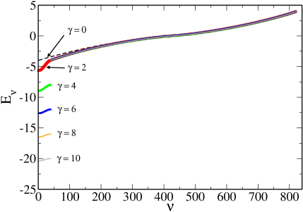
Figure 1: Energy spectrum of the two-boson BH chain with fixed boundary conditions for different values of the interaction strength $\gamma$. The eigenvalues are plotted as a function of the eigenvalue label (see text). Here $f=40$.

In Fig. 1 we show the energy spectrum of the Hamiltonian matrix (13) obtained by numerical diagonalization for different values of the interaction parameter $\gamma$. In all calculations by numerical diagonalization we used $f=40$, which leads to a matrix dimension $d=820$. The eigenstates are ordered with respect to their eigenvalues $E_{\nu}$ ($\nu=1,\ldots,d$). At $\gamma=0$, the spectrum consists of the two-boson continuum, whose eigenstates $|k_{1},k_{2}\rangle$ are given by (10). The eigenenergies are the sum of the two single-particle energies:

$$E_{k_{1},k_{2}}^{0}=-2[\cos(k_{1})+\cos(k_{2})].$$ (17)

When $\gamma>0$, eigenvalues in the lower part of the spectrum are pushed down, and beyond $\gamma\approx 2$ a band of $f$ states splits off from the two-boson continuum. These are the two-boson bound states, with a high probability of finding the two bosons on the same lattice site, while the probability of them being separated by a distance $r$ decreases exponentially with increasing $r$ [16, 15, 14].

The critical value $\gamma_{b}=2$ for which the band of two-boson bound states splits off from the continuum may be explained as follows. In the limit $f\to\infty$ the unnormalized bound state with highest energy $E=-2\gamma$ is given by [14, 17]:

$$|\Psi\rangle=\sum_{l=1}^{f}(-1)^{l}|l,l\rangle.$$ (18)

For $\gamma_{b}=2$ the energy of that state leaves the two-boson continuum of energies $E\in[-4,4]$.

3 Localization in normal-mode space

We recall that the normal-mode space is spanned by both momenta $k_{1}$ and $k_{2}$. The conditions $0<k_{1,2}<\pi$ and $k_{1}\leq k_{2}$ reduce the normal-mode space to a triangle that we call the irreducible triangle, as sketched in Fig. 2. For finite $f$ and $\gamma$ the eigenstates $|\Psi\rangle$ will spread in the basis of the $\gamma=0$ eigenstates $\{|k_{1},k_{2}\rangle\}$. We measure such a spreading by computing the weight function in normal-mode space $C(k_{1},k_{2})=|\langle k_{1},k_{2}|\Psi\rangle|^{2}$.

3.1 Analysis by perturbation theory

We use perturbation theory to calculate the weight functions, where $\gamma$ is the perturbation. We fix the momentum $k_{1}$ and $k_{2}$, and choose an eigenstate $|\tilde{k}_{1},\tilde{k}_{2}\rangle$ of the unperturbed case $\gamma=0$. The wave numbers $\tilde{k}_{1}$ and $\tilde{k}_{2}$ define a seed point $P=(\tilde{k}_{1},\tilde{k}_{2})$ in the irreducible triangle (see Fig. 2). Upon increase of $\gamma$, the chosen eigenstate transforms into a new eigenstate $|\Psi_{\tilde{k}_{1}\tilde{k}_{2}}\rangle$, which will have overlap with several eigenstates of the $\gamma=0$ case. We expand the eigenfunction of the perturbed system to first order in $\gamma$:

$$|\Psi_{\tilde{k}_{1}\tilde{k}_{2}}\rangle=|\tilde{k}_{1},\tilde{k}_{2}\rangle+\gamma|\Psi_{\tilde{k}_{1},\tilde{k}_{2}}^{(1)}\rangle,$$ (19)

where

$$|\Psi_{\tilde{k}_{1},\tilde{k}_{2}}^{(1)}\rangle=\sum_{k^{\prime}_{1}\neq\tilde{k}_{1}}\sum_{\begin{subarray}{c}k^{\prime}_{2}\neq\tilde{k}_{2}\\ k^{\prime}_{2}\geq k^{\prime}_{1}\end{subarray}}\frac{\langle k^{\prime}_{1},k^{\prime}_{2}|\hat{H}_{1}|\tilde{k}_{1},\tilde{k}_{2}\rangle}{{E_{{\tilde{k}_{1}}{\tilde{k}_{2}}}^{0}}-E_{{{k}_{1}^{\prime}}{k_{2}^{\prime}}}^{0}}|k^{\prime}_{1},k^{\prime}_{2}\rangle.$$ (20)

Thus for $k_{1}\neq\tilde{k}_{1}$ and $k_{2}\neq\tilde{k}_{2}$ the weight function $C(k_{1},{k}_{2};{\tilde{k}_{1}},\tilde{k}_{2})=|\langle k_{1},k_{2}|\Psi_{\tilde{k}_{1}{\tilde{k}_{2}}}\rangle|^{2}$ is

$$C(k_{1},{k}_{2};{\tilde{k}_{1}},\tilde{k}_{2})=\gamma^{2}\frac{|\langle k_{1},k_{2}|\hat{H}_{1}|\tilde{k}_{1},\tilde{k}_{2}\rangle|^{2}}{|E_{{\tilde{k}_{1}}{\tilde{k}_{2}}}^{0}-E_{{k}_{1}{k}_{2}}^{0}|^{2}},$$ (21)

where $E_{k_{1}k_{2}}^{0}$ and $E_{\tilde{k}_{1}\tilde{k}_{2}}^{0}$ are eigenenergies of the unperturbed system given by (17). For convenience we use new variables in normal-mode space

$$k_{\pm}=k_{2}\pm k_{1},$$ (22)

which are the total (Bloch) and relative wave numbers respectively. They have values $0<k_{+}<2\pi$ and $0<k_{-}<\pi$. Since we are interested in the behavior of the weight function around the core at $(\tilde{k}_{1},\tilde{k}_{2})$, we define the coordinates relative to that point:

$$\Delta_{\pm}={k}_{\pm}-\tilde{k}_{\pm}.$$ (23)

Thus, (21) becomes

$$C(k_{1},k_{2};\tilde{k}_{1},\tilde{k}_{2}) = \gamma^{2}\frac{f_{q_{1},q_{2},\tilde{q}_{1},\tilde{q}_{2}}^{2}}{[16(E_{\tilde{k}_{1}\tilde{k}_{2}}^{0}-E_{k_{1}k_{2}}^{0})]^{2}}$$ (24)

$$\;\;\;\;\;\;\;\;\;\;\;\;\;\times\;R_{k_{+},k_{-};\tilde{k}_{+},\tilde{k}_{-}}^{2},$$

where $f_{q_{1},q_{2},\tilde{q}_{1},\tilde{q}_{2}}$ is given by Eq. (16).

The coefficient $R_{k_{+},k_{-};\tilde{k}_{+},\tilde{k}_{-}}$ consists of a sum of eight terms of the form

$$g(\zeta)=\frac{\sin\left[(2f+1)\frac{\zeta}{2}\right]}{\sin\left(\frac{\zeta}{2}\right)},$$ (25)

with pairwise opposite signs (see appendix A). For each term, the argument $\zeta$ is a certain combination of the wave numbers $k_{+},k_{-}$ and $\tilde{k}_{+},\tilde{k}_{-}$ (see appendix A for details). Unless the argument of any of the eight terms $g(\zeta)$ vanishes, all of them cancel each other and $R_{k_{+},k_{-};\tilde{k}_{+},\tilde{k}_{-}}=0$. Thus the condition $\zeta=0$ for each term in $R_{k_{+},k_{-};\tilde{k}_{+},\tilde{k}_{-}}$, together with the relations (22) and (23), defines lines $k_{2}=k_{2}(k_{1})$ in the normal-mode space where the weight function $C(k_{1},k_{2};\tilde{k}_{1},\tilde{k}_{2})$ is nonzero. These lines are schematically shown in Fig. 2 (the analytical derivation of these lines is given in appendix A). Note that these lines are specularly reflected at the boundaries $k_{1}=0$ and $k_{2}=\pi$ of the irreducible triangle.

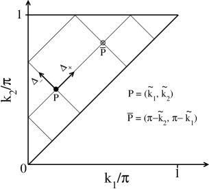
Figure 2: Sketch of the different lines in the two-dimensional normal-mode space along which the weight function (21) is nonzero. The seed point $P=(\tilde{k}_{1},\tilde{k}_{2})$ corresponding to the unperturbed eigenstate $|\tilde{k}_{1},\tilde{k}_{2}\rangle$ is represented by the black spot. Its conjugate point $\bar{P}=(\pi-\tilde{k}_{2},\pi-\tilde{k}_{1})$ is represented by the grey spot. The axes defining the coordinates $\Delta_{+}$ and $\Delta_{-}$ are indicated by the arrows emerging from $P$.

To study the localization in normal-mode space away from the core using the formula (24), we consider the two cases $\Delta_{-}=0$, $\Delta_{+}>0$ and vice versa, i.e. the mutually perpendicular directions $\Delta_{+}$ and $\Delta_{-}$ (Fig. 2). For each case we obtain, with $|\Delta_{\pm}|\ll\pi$,

$$C^{\pm}(k_{1},{k}_{2};{\tilde{k}_{1}},\tilde{k}_{2}) = \left(\frac{\gamma}{f+1}\right)^{2}(2-{\delta}_{q_{1},q_{2}})(2-{\delta}_{\tilde{q}_{1},\tilde{q}_{2}})$$ (26)

$$\times \Delta_{\pm}^{-2}\Bigg{\{}\left[\cos(\tilde{k}_{1})+\cos(\tilde{k}_{2})\right]\frac{\Delta_{\pm}}{2}$$

$$+ \sin(\tilde{k}_{1})\pm\sin(\tilde{k}_{2})\Bigg{\}}^{-2}.$$

The effective interaction strength is $\gamma/(f+1)$. In the limit $\gamma\to 0$ or $f\to\infty$ we have compactification of the eigenstates. The formula (26) shows localization in normal-mode space. Depending on the seed $(\tilde{k}_{1},\tilde{k}_{2})$ we find algebraic decay within the irreducible triangle, $C\sim\Delta^{-\alpha}$, with $\alpha=2,4$. If $\sin\tilde{k}_{1}\pm\sin\tilde{k}_{2}\neq 0$, $\alpha=2$. If $\sin\tilde{k}_{1}\pm\sin\tilde{k}_{2}=0$, $\alpha=4$. E.g. for $\tilde{k}_{1}=\tilde{k}_{2}$

$$C^{-}\sim\left(\frac{\gamma}{f+1}\right)^{2}\frac{1}{\cos^{2}(\tilde{k}_{1})\Delta_{-}^{4}}.$$ (27)

Note that along the $\Delta_{+}$ direction in the irreducible triangle, $R_{k_{+},k_{-};\tilde{k}_{+},\tilde{k}_{-}}=2(f+1)$ at all points but $\bar{P}=(\bar{k}_{1}=\pi-\tilde{k}_{2},\bar{k}_{2}=\pi-\tilde{k}_{1})$. This is the conjugate point of the seed $P$ (Fig. 2), where two lines intersect. At this point $R_{k_{+},k_{-};\tilde{k}_{+},\tilde{k}_{-}}=4(f+1)$. Thus we expect a local maximum of the weight function at the conjugate point. The states $|\tilde{k}_{1},\tilde{k}_{2}\rangle$ and $|\bar{k}_{1},\bar{k}_{2}\rangle$ have energies $E_{\bar{k}_{1},\bar{k}_{2}}^{0}=-E_{\tilde{k}_{1},\tilde{k}_{2}}^{0}$.

3.2 Numerical results

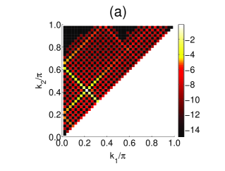
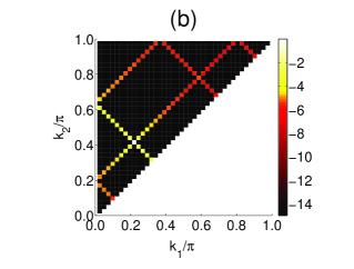
Figure 3: 3-D plot of the logarithm of the weight function in the normal-mode space for the eigenstate $\nu=145$, obtained by (a) numerical diagonalization, and (b) perturbation theory using the formula (24). Here $f=40$ and $\gamma=0.1$.

In Fig. 3 we show the weight function in the two-dimensional normal-mode space obtained by numerical diagonalization and the formula (24) respectively, with characteristic localization profiles. We find agreement of the numerical data with the results from perturbation theory. The largest value is at the point $P=(\frac{9}{40}\pi,\frac{17}{40}\pi)\sim(0.2\pi,0.4\pi)$, and it decays mainly along the lines described in the previous section (Fig. 2). Note also the presence of the local maximum at the conjugate point $\bar{P}\sim(0.6\pi,0.8\pi)$ in both cases.

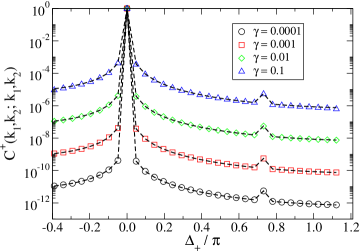
Figure 4: Weight function for different values of the interaction strength $\gamma$ of the eigenstate $\nu=145$ along the $\Delta_{+}$ direction. The dashed lines are results from formula (24). Here $f=40$.

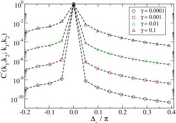
Figure 5: Weight function for different values of the interaction strength $\gamma$ of the eigenstate $\nu=145$ along the $\Delta_{-}$ direction. The dashed lines are results from formula (24). Here $f=40$.

In Figs. 4 and 5 we plot the weight function of the eigenstate shown in Fig. 3 along the directions $\Delta_{+}$ and $\Delta_{-}$ respectively for different values of the interaction parameter $\gamma$. The state becomes less localized with increasing $\gamma$, as expected from the above analysis. The decay of the weight function is well described by perturbation theory (dashed lines). The peak of the weight function at the conjugate point is clearly seen in Fig. 4.

In Fig. 6 we plot the weight function of different states along the $\Delta_{+}$ direction. It decays as a power law that ranges from $\Delta^{-4}$ for states near the lower corner of the irreducible triangle (see Fig. 8) to $\Delta^{-2}$ for states fulfilling $\tilde{k}_{2}\approx\pi-\tilde{k}_{1}$. In Fig. 7 we plot the decay of the weight function along the $\Delta_{-}$ direction, where we see the power-law decay that ranges from $\Delta^{-4}$ for states fulfilling $\tilde{k}_{1}\approx\tilde{k}_{2}$ (see Fig. 8), to $\Delta^{-2}$ for states fulfilling $\tilde{k}_{2}\approx\pi-\tilde{k}_{1}$. The results from numerical diagonalization agree very well with those from the perturbation theory analysis.

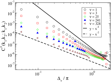
Figure 6: Weight function of different eigenstates (labeled by the index $\nu$) along the $\Delta_{+}$ direction. Here $\gamma=0.1$ and $f=40$.

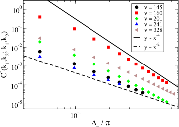
Figure 7: Weight function of different eigenstates (labeled by the index $\nu$) along the $\Delta_{-}$ direction. Here $\gamma=0.1$ and $f=40$.

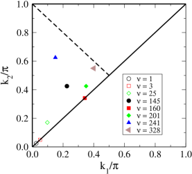
Figure 8: Location $P=(\hat{k}_{1},\hat{k}_{2})$ of the eigenstates, shown in Figs. 6 and 7, in the irreducible triangle.

3.3 Nonperturbative effects

The results in the previous section were obtained for small values of the interaction parameter $\gamma$ up to $\gamma=0.1$, for which perturbation theory gives a good description of the results obtained by numerical diagonalization. However, when increasing $\gamma$ several nonperturbative effects occur. These are:

Split off of the two-boson bound state band: This effect was discussed in Sec. 2.2 (Figs. 1). When $\gamma>2$ the two-boson bound state band splits off from the two-boson continuum, and the corresponding eigenstates are correlated in direct space, i.e. with large probability the two bosons are occupying identical lattice sites. Thus, in normal-mode space these eigenstates become delocalized as shown in Fig. 9.

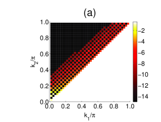
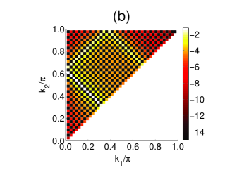
Figure 9: 3-D plot of the logarithm of the weight function in normal-mode space for the eigenstate $\nu=25$, that belongs to the two-boson bound state band. Results were obtained by numerical diagonalization. (a) $\gamma=1.5$. The two-boson bound state band did not split off and the eigenstate is localized in normal-mode space. (b) $\gamma=2$. At this interaction value the two-boson bound state band splits off and the eigenstate becomes delocalized in normal-mode space. Here $f=40$.

Degenerate levels in the noninteracting case: The analysis using perturbation theory is valid as long as the eigenstate which is continued from the noninteracting case is not degenerate. Because of the finiteness of the lattice the momenta $\tilde{k}_{1}$ and $\tilde{k}_{2}$ are restricted to discrete values and define a grid in the two-dimensional normal-mode space. A grid point $(\tilde{k}_{1},\tilde{k}_{2})$ defines a line of constant energy in normal-mode space through Eq. (17), with $E_{k_{1},k_{2}}^{0}=E_{\tilde{k}_{1},\tilde{k}_{2}}^{0}$ (Fig. 10-a). The nondegeneracy condition implies that this line should not pass through any other grid point. It is easy to see from Eq. (17) that all states $|\tilde{k}_{1},\pi-\tilde{k}_{1}\rangle$ are degenerate, with $E_{\tilde{k}_{1},\pi-\tilde{k}_{1}}=0$. Their corresponding grid points in the irreducible triangle lie on the diagonal $k_{2}=\pi-k_{1}$ (thick line in Fig. 10-a). In Fig. 10-b we show the weight function of an eigenstate that is located on that diagonal in the noninteracting case. As expected, even for small values of $\gamma$, the state completely delocalizes along the degeneracy diagonal.

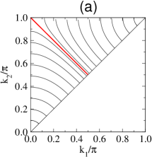
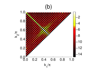
Figure 10: (a) Lines of constant energy given by (17). The red thick line is the $E_{k_{1},k_{2}}^{0}=0$-line where all unperturbed states $|k_{1},k_{2}=\pi-k_{1}\rangle$ are degenerate. (b) 3-D plot of the logarithm of the weight function in normal-mode space for the eigenstate $\nu=405$, obtained by numerical diagonalization with $\gamma=0.1$ and $f=40$. In the noninteracting case this state corresponds to $|k_{1},k_{2}=\pi-k_{1}\rangle$.

Avoided crossings: Upon increase of the interaction parameter $\gamma$, the energies of continued eigenstates change, and will resonate with eigenvalues of other states.

The first possible avoided level crossing defines a critical value of the interaction parameter $\gamma$ up to which first-order perturbation theory is applicable. To estimate this value, $\gamma_{c}$, we assume that before the first avoided crossing is encountered, the eigenenergies depend linearly on $\gamma$. This dependence may be estimated using first-order perturbation theory in $\gamma$. The result is, for large $f$,

$$E_{\tilde{k}_{1},\tilde{k}_{2}}(\gamma)\approx E_{\tilde{k}_{1},\tilde{k}_{2}}^{0}+\frac{b(\tilde{k}_{1},\tilde{k}_{2})}{f}\gamma,$$ (28)

where

$$b(\tilde{k}_{1},\tilde{k}_{2})=\left\{\begin{array}[]{ll}2&\textrm{if $\tilde{k}_{1}=0$},\\ -2&\textrm{if $\tilde{k}_{2}=\tilde{k}_{1}>0$},\\ -1&\textrm{if $\tilde{k}_{1}>0,\;\tilde{k}_{2}>\tilde{k}_{1}$.}\end{array}\right.$$ (29)

Let us consider two levels $E_{1}$ and $E_{2}$ that interact in the first avoided level crossing. At $\gamma=0$ they are separated by $\delta E$. For nonzero $\gamma$ the energies linearly change in $\gamma$:

$$E_{1}=E_{\tilde{k}_{1},\tilde{k}_{2}}^{0}+\frac{|b_{1}(\tilde{k}_{1},\tilde{k}_{2})|}{f}\gamma,$$ (30)

$$E_{2}=E_{\tilde{k}_{1},\tilde{k}_{2}}^{0}+\delta E-\frac{|b_{2}(\tilde{k}_{1},\tilde{k}_{2})|}{f}\gamma.$$ (31)

By equating $E_{1}$ and $E_{2}$ at $\gamma=\gamma_{c}$ we obtain

$$\gamma_{c}(\tilde{k}_{1},\tilde{k}_{2})=\frac{f\delta E}{|b_{1}(\tilde{k}_{1},\tilde{k}_{2})|+|b_{2}(\tilde{k}_{1},\tilde{k}_{2})|}.$$ (32)

The first avoided crossing of the level $E_{1}$ will happen with its nearest neighbor in the spectrum of the $\gamma=0$ case, which is separated by $\delta E(\tilde{k}_{1},\tilde{k}_{2})$. Using Eq. (17) with $\tilde{k}_{1},\tilde{k}_{2}\ll\pi/2$ (see Fig. 10-a), the separation is estimated (see appendix B): $\delta E\approx 4\sqrt{2}\pi/(f+1)^{2}$. Therefore $\gamma_{c}\sim 1/f$.

The coefficient $b_{1}(\tilde{k}_{1},\tilde{k}_{2})$ depends on the state $|\tilde{k}_{1},\tilde{k}_{2}\rangle$ under consideration through (29). The coefficient $b_{2}(\tilde{k}_{1},\tilde{k}_{2})$ must have opposite sign as compared to $b_{1}(\tilde{k}_{1},\tilde{k}_{2})$ for the avoided crossing to take place. For the states $\nu=145$ and $\nu=41$ located at $(\tilde{k}_{1},\tilde{k}_{2})\approx(0.2\pi,0.4\pi)$ and $(\tilde{k}_{1},\tilde{k}_{2})\approx(0.12\pi,0.22\pi)$ respectively (see Fig. 8), $b_{1}(\tilde{k}_{1},\tilde{k}_{2})=-1$ and $b_{2}(\tilde{k}_{1},\tilde{k}_{2})=2$. This leads to a critical value of the interaction parameter $\gamma_{c}\approx 0.28$, which is in reasonable agreement with the numerical results: $\gamma_{c}\approx 0.2$ for the state $\nu=145$, and $\gamma_{c}\approx 0.3$ for the state $\nu=41$.

4 Conclusions

In this work we studied the properties of quantum q-breathers in a one-dimensional lattice containing two bosons modeled by the BH Hamiltonian with fixed boundary conditions. Because of the lack of translational invariance, the normal-mode space is two-dimensional and reduces to a triangle when working in the irreducible representation of the product basis states (the irreducible triangle). To explore localization phenomena in this system we computed appropriate weight functions of the eigenstates in the normal-mode space using both perturbation theory and numerical diagonalization. We find that the weight function is sizable only along the mutually perpendicular directions defined by the total and relative momentum, thus it defines lines in the irreducible triangle that show specular reflections at the boundaries of the irreducible triangle. We observe localization of the weight function along these lines. The localization is stronger when the size of the system increases or the interaction parameter is weaker, the former because the effective interaction drops in the dilute limit of large chains. We found algebraic localization. The power of the decay is different for each eigenstate depending on which seed wave numbers have in the noninteracting case, ranging from two to four.

An interesting effect is the local maximum of the weight function at the symmetry-related (conjugate) point of the eigenstate core in normal-mode space, due to a crossing between different paths described by the lines along which the weight function is nonzero within perturbation theory.

In addition to the existence of degeneracies between eigenstates in the noninteracting case, we analyzed other nonperturbative effects as the interaction parameter increases, which limit the applicability of perturbation theory to describe the system: The splitting off of the two-boson bound states from the two-boson continuum, and the occurrence of avoided level crossings. The first effect manifests as a delocalization of the weight function of the bound states due to the two-boson correlation in direct space. The second effect manifests as a sudden change of the location of an eigenstate in the normal-mode space due to resonant interaction with another eigenstate. Both effects define critical values of the interaction parameter below which one may analyze the system by perturbation theory. The occurrence of an avoided level crossing gives the smallest critical value.

Although we considered a system with fixed boundary conditions, we still obtain algebraic decay as in the case with periodic boundary conditions [14]. The question how to restore exponential localization of classical q-breathers from algebraic decay of quantum q-breathers in the limit of large numbers of particles is still open. When going to that limit, one may use a Hartree approximation and describe the system with a product state wavefunction, or use a coherent state representation. Both ways lead to the nonlinear Schrödinger equation where classical q-breathers are known to exist [12].

Appendix A Lines of nonzero weight function

For fixed $\tilde{k}_{1},\tilde{k}_{2}$, the coefficient $R(k_{1},k_{2};\tilde{k}_{1},\tilde{k}_{2})$ in Eq. (24) is given by

$$R(k_{1},k_{2};\tilde{k}_{1},\tilde{k}_{2}) = g(k_{-}+\tilde{k}_{-})+g(\Delta_{-})$$ (33)

$$- g(k_{-}+\tilde{k}_{+})-g(k_{-}-\tilde{k}_{+})$$

$$- g(k_{+}+\tilde{k}_{-})-g(k_{+}-\tilde{k}_{-})$$

$$+ g(\Delta_{+})+g(k_{+}+\tilde{k}_{+}),$$

where

$$g(\zeta)=\frac{\sin[(2f+1)\frac{\zeta}{2}]}{\sin(\frac{\zeta}{2})}.$$ (34)

The lines $k_{2}=k_{2}(k_{1})$ in the normal-mode space (irreducible triangle) along which $R(k_{1},k_{2};\tilde{k}_{1},\tilde{k}_{2})\neq 0$ are obtained from the condition that the argument of any term in (33) is zero, such that

$$g(\zeta)=2f+1.$$ (35)

Let us analyze each of the arguments in Eq. (33):

• $k_{-}+\tilde{k}_{-}=0$: This implies that

  $$k_{2}-k_{1}=-(\tilde{k}_{2}-\tilde{k}_{1}).$$ (36)

  Since $k_{2}\geq k_{1}$ the above condition is possible only for points $(\tilde{k}_{1},\tilde{k}_{2}),(k_{1},k_{2})$ on the diagonal $k_{2}=k_{1}$.

• $\Delta_{-}=0$: This condition leads to

  $$k_{2}=(\tilde{k}_{2}-\tilde{k}_{1})+k_{1},$$ (37)

  which is the equation of the line along the $\Delta_{+}$ direction that cuts the $k_{2}$ axis at $k_{2}(0)=\tilde{k}_{2}-\tilde{k}_{1}$.

• $k_{-}+\tilde{k}_{+}=0$: This implies that

  $$k_{2}-k_{1}=-(\tilde{k}_{2}+\tilde{k}_{1}),$$ (38)

  which is possible only if $\tilde{k}_{1}=\tilde{k}_{2}=0$ and $(k_{1},k_{2})$ is on the diagonal $k_{2}=k_{1}$.

• $k_{-}-\tilde{k}_{+}=0$: This leads to the equation

  $$k_{2}=(\tilde{k}_{2}+\tilde{k}_{1})+k_{1},$$ (39)

  which describes a line parallel to the $\Delta_{+}$ direction that cuts the $k_{2}$ axis at $k_{2}(0)=\tilde{k}_{2}+\tilde{k}_{1}$.

• $k_{+}+\tilde{k}_{-}=0$: This implies that

  $$k_{2}=-(\tilde{k}_{2}+\tilde{k}_{1})-k_{1},$$ (40)

  which is valid only if $k_{1}=k_{2}=\tilde{k}_{1}=\tilde{k}_{2}=0$.

• $k_{+}-\tilde{k}_{-}=0$: This leads to the equation

  $$k_{2}=(\tilde{k}_{2}-\tilde{k}_{1})-k_{1},$$ (41)

  which is the equation of a line parallel to the $\Delta_{-}$ direction that cuts the $k_{2}$ axis at $k_{2}(0)=\tilde{k}_{2}-\tilde{k}_{1}$.

• $\Delta_{+}=0$: This leads to the equation

  $$k_{2}=(\tilde{k}_{2}+\tilde{k}_{1})-k_{1},$$ (42)

  which describes the line along to the $\Delta_{-}$ direction that cuts the $k_{2}$ axis at $k_{2}(0)=\tilde{k}_{2}+\tilde{k}_{1}$.

Appendix B Energy separation between nearest-neighbor levels in the noninteracting case

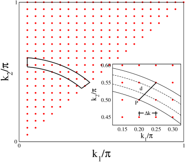
Figure 11: Sketch of the discrete normal-mode space (irreducible triangle) with a line of constant energy in the circular approximation passing through the grid point $P=(\tilde{k}_{1},\tilde{k}_{2})$ and the grid point $(\tilde{k}_{1}+\Delta k,\tilde{k}_{2}+\Delta k)$. The strip of width $d=\sqrt{2}\Delta k$ and area $A_{s}$ contains $N_{g}=A_{s}/\Delta k^{2}$ grid points through which lines of constant energy pass. The typical line separation within the strip is $\delta k\approx d/N_{g}$. $\Delta k=\pi/(f+1)$ is the grid spacing.

The finite size of the lattice leads to discrete values of the momenta $k_{1}$ and $k_{2}$, and thus to a grid in the normal-mode space (Fig. 11). Let us consider a line of constant energy which passes through the seed point $P=(\tilde{k}_{1},\tilde{k}_{2})$ given by $E_{k_{1},k_{2}}^{0}=E_{\tilde{k}_{1},\tilde{k}_{2}}^{0}$ with Eq. (17). For small values of $k_{1}$ and $k_{2}$, the energy in Eq. (17) may be approximated to

$$E_{k_{1},k_{2}}^{0}\approx-4+k_{1}^{2}+k_{2}^{2},$$ (43)

which is the equation for a circle (circular approximation). So the equation for the line of constant energy passing through the point $P$ is

$$k_{2}(k_{1};\tilde{k}_{1},\tilde{k}_{2})=\sqrt{\tilde{k}_{1}^{2}+\tilde{k}_{2}^{2}-k_{1}^{2}}.$$ (44)

Through another grid point at $(\tilde{k}_{1}+\Delta k,\tilde{k}_{2}+\Delta k)$, separated from $P$ by a distance $d=\sqrt{2}\Delta k\approx\Delta k$ ($\Delta k$ is the grid spacing), another line of constant energy with the form (44) passes (Fig. 11), defining a strip of area $A_{s}$ in the irreducible triangle. The strip contains $N_{g}$ grid points through which lines of constant energy pass. The average line separation within the strip is $\delta k\approx d/N_{g}$.

The number of grid points in the strip is

$$N_{g}=\frac{A_{s}}{\Delta k^{2}}.$$ (45)

The area of the strip is

$$A_{s} = \frac{\pi}{8}[(\tilde{k}_{1}+\Delta k)^{2}+(\tilde{k}_{2}+\Delta k)^{2}-\tilde{k}_{1}^{2}-\tilde{k}_{2}^{2}]$$ (46)

$$= \frac{\pi}{4}[\Delta k^{2}+(\tilde{k}_{1}+\tilde{k}_{2})\Delta k].$$

Therefore

$$N_{g}=\frac{\pi}{4\Delta k}(\Delta k+\tilde{k}_{1}+\tilde{k}_{2}),$$ (47)

and hence

$$\delta k(\tilde{k}_{1},\tilde{k}_{2})=\frac{4\Delta k^{2}}{\pi(\tilde{k}_{1}+\tilde{k}_{2}+\Delta k)}.$$ (48)

The corresponding energy separation is

$$\delta E(\tilde{k}_{1},\tilde{k}_{2})=E_{\tilde{k}_{1}+\delta k_{1},\tilde{k}_{2}+\delta k_{2}}^{0}-E_{\tilde{k}_{1},\tilde{k}_{2}}^{0},$$ (49)

with $\delta k_{1}=\delta k_{2}=\delta k/\sqrt{2}$. Substituting (43) and (48) into (49) one obtains

$$\delta E(\tilde{k}_{1},\tilde{k}_{2}) = \frac{16\Delta k^{4}}{\pi^{2}(\tilde{k}_{1}+\tilde{k}_{2}+\Delta k)^{2}}+$$ (50)

$$\frac{4\sqrt{2}(\tilde{k}_{1}+\tilde{k}_{2})\Delta k^{2}}{\pi(\tilde{k}_{1}+\tilde{k}_{2}+\Delta k)}.$$

For $f$ large, and $\Delta k=\pi/(f+1)\ll\tilde{k}_{1,2}$, the first term in (50) can be neglected. Thus we are left with

$$\delta E(\tilde{k}_{1},\tilde{k}_{2})\approx\frac{4\sqrt{2}\pi}{(f+1)^{2}}.$$ (51)

References

• [1] S. Flach, C.R. Willis, Phys. Rep. 295, 181 (1998); S. Flach and A. V. Gorbach, Phys. Rep. 467, 1 (2008).
• [2] D. K. Campbell, S. Flach, Y. S. Kivshar, Phys. Today 57(1), 43 (2004).
• [3] A. J. Sievers, J. B. Page, in: G. K. Horton, A. A. Maradudin (eds.), Dynamical Properties of Solids VII, Phonon Physics. The Cutting Edge, Elsevier, Amsterdam (1995), p. 137.
• [4] S. Aubry, Physica D 103, 201 (1997).
• [5] E. Fermi, J. Pasta, and S. Ulam, Los Alamos Report $N^{\circ}$ LA-1940, 1955; in Collected Papers of Enrico Fermi, edited by E. Segre (University of Chicago Press, Chicago, 1965), Vol. II, pp. 977-978; Many Body Problems, edited by D. C. Mattis (World Scientific, Singapore, 1993).
• [6] S. Flach, M. V. Ivanchenko and O. I. Kanakov, Phys. Rev. Lett. 95, 064102 (2005).
• [7] M. V. Ivanchenko, O. I. Kanakov, K. G. Michagin, and S. Flach, Phys. Rev. Lett. 97, 025505 (2006).
• [8] S. Flach, M. V. Ivanchenko, and O. I. Kanakov, Phys. Rev. E 73, 036618 (2006).
• [9] O. I. Kanakov, S. Flach, M. V. Ivanchenko and K. G. Mishagin, Phys. Lett. A 365, 416 (2007).
• [10] T. Penati and S. Flach, Chaos 17, 023102 (2007).
• [11] S. Flach and A. Ponno, Physica D 237, 908 (2008).
• [12] K. G. Mishagin, S. Flach, O. I. kanakov and M. V. Ivanchenko, New J. Phys. 10, 073034 (2008).
• [13] S. Flach, M. V. Ivanchenko, O. I. Kanakov and K. G. Mishagin, Am. J. Phys. 76, 453 (2008).
• [14] J. P. Nguenang, R. A. Pinto, S. Flach. Phys.Rev.B 75, 214303 (2007).
• [15] A. C. Scott, Nonlinear Science (Oxford University Press, Oxford, 1999).
• [16] A. C. Scott, J. C. Eilbeck and H. GilhΓΈj, Physica D 78, 194 (1994).
• [17] J. C. Eilbeck, in: Localization and Energy Transfer in Nonlinear Systems, Ed. L. Vazquez, R. S. MacKay and M. P. Zorzano, p.177 (World Scientific, Singapore 2003).
• [18] M. H. Cohen, and J. Ruvalds, Phys. Rev. Lett. 23, 1378 (1969).
• [19] J. C. Kimball, C. Y. Fong, and Y. R. Shen, Phys. Rev. B 23, 4946 (1981).
• [20] L. J. Richter, T. A. Germer, J. P. Sethna, and W. Ho, Phys. Rev. B 38, 10403 (1988).
• [21] P. Guyot-Sionnest, Phys. Rev. Lett. 67, 2323 (1991).
• [22] D. J. Dai, and G. E. Ewing, Surf. Sci. 312, 239 (1994).
• [23] R. P. Chin, X. Blase, Y. R. Shen, and S. G. Louie, Europhys. Lett. 30, 399 (1995).
• [24] P. Jakob, Phys. Rev. Lett. 77, 4229 (1996).
• [25] P. Jakob, Appl. Phys. A: Mater. Sci. Process. 75, 45 (2002).
• [26] V. Pouthier, J. Chem. Phys. 118, 9364 (2003).
• [27] H. Okuyama, T. Ueda, T. Aruga, and M. Nishijima, Phys. Rev. B 63, 233404 (2001).
• [28] V. Pouthier, Phys. Rev. E 68, 021909 (2003).
• [29] J. Edler, R. Pfister, V. Pouthier, C. Falvo, and P. Hamm, Phys. Rev. Lett. 93, 106405 (2004).
• [30] L. Proville, Europhys. Lett. 69, 763 (2005).
• [31] L. Proville, Phys. Rev. B 71, 104306 (2005).
• [32] Z. IviΔ‡, G. P. Tsironis, Physica D 216, 200 (2006).
• [33] K. Winkler, G. Thalhammer, F. Lang, R. Grimm, J. Ecker Denshlag, A. J. Daley, A. Kantian, H. P. BΓΌchler, and P. Zoller, Nature 441, 853 (2006).