Sensitivity of p modes for constraining velocities of microscopic diffusion of the elements

Abstract

Conventional astrophysical observations have failed to provide stringent constraints on physical processes operating in the interior of the stars. However, satellite missions now promise a solution to these problems by providing long-term high-quality continuous data which will allow the application of seismic techniques. With this in mind, and using the Sun as our astrophysical laboratory, our aim is to determine if Corot- and Kepler-like asteroseismic data can constrain physical processes like microscopic diffusion. We test to what extent can the observed atmospheric abundances coupled with p-mode frequencies safely distinguish between stellar initial chemical composition and diffusion of these elements. We present some preliminary results of our analysis.

Instituto de Astrofísica de Canarias, C/ Vía Lactea s/n, La Laguna 38205, Tenerife, Spain: Email: orlagh@iac.es

Indian Institute of Astrophysics, Koramangala, Bangalore 560034, India

Laboratoire AIM, CEA/DSM-CNRS-Université Paris Diderot; CEA, IRFU, SAp, F-91191, Gif-sur-Yvette, France

1. Introduction & Method

If we have the following observations for a solar-type star: a set of p-mode frequencies, measured abundances, and an identified g mode, we can investigate how these observations may constrain some of the physical processes occuring in the interior of a star. Suppose that the stellar model is a main sequence 1 M_⊙ star, and that we can calibrate the age of the star using the radius and luminosity. Then the free parameters that remain to be fitted in the star are the initial mass fractions of hydrogen and metals $X_{0}$ and $Z_{0}$, and the velocities of diffusion of these elements $V_{X}$, $V_{Y}$ and $V_{Z}$, (assuming that other microscopic processes may not be “observable”), where $Y$ denotes helium. Let’s denote these set of parameters as P. Using P we can calculate a stellar model which will give us the expected observables, B (expected p-mode frequencies, abundances etc.). If we have a set of observations O, then in order to find the P that most adequately reproduce O, we can use the following equation iteratively, until we make O as close as possible to B:

$$\boldmath\delta{\bf P=V}{\bf{\tilde{W}}^{-1}}{\bf U}\frac{{\bf O-B}}{\epsilon}.\unboldmath$$ (1)

$\delta$P are the parameter corrections to make to the initial guess P₀, $\epsilon$ are the measurement errors, and UWV^T is the singular value decomposition of the sensitivity matrix, which can be written as $\frac{\partial B}{\partial P}/\epsilon$ and $\tilde{{\bf W}^{-1}}$ has some zero values to stabilize the inversion (see Creevey (2008, 2009)).

Once P have been found, then the theoretical uncertainties $\sigma$(P) can be calculated for each $j=1,2,...N$ parameter

$$\boldmath\sigma_{j}^{2}({\bf P})=\sum_{k}^{N}\frac{{\bf V}_{jk}^{2}}{{\bf\tilde{W}}_{k}^{2}}.\unboldmath$$ (2)

The partial derivatives were calculated using the CESAM code Code d’Evolution Stellaire Adaptatif et Modulaire (Morel 1997) and ADIPLS (Christensen-Dalsgaard 2007). We took the standard solar model as a reference using the abundances of Grevesse & Noels (1993), and calibrated these models in radius and luminosity to an accuracy of $\sim 10^{-2}$ as described in Mathur et al. (2007). The reference parameters for the models are $(X_{0},Z_{0})=(0.708,0.0195)$ and $(V_{X},V_{Y},V_{Z})=(2.307,-7.063,-5.635)\times 10^{-9}$ cm s^-1.

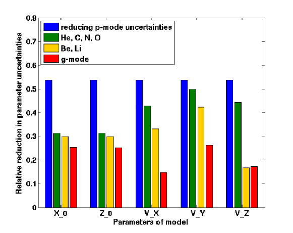
Figure 1.: The relative uncertainties as a fraction of the initial values of 3%, 24%, 189%, 217%, 422% (details in text) as extra observables are included.

2. Results and Discussion

2.1. Impact of each observable on the uncertainties

Using only p-mode frequencies to determine the parameter uncertainties (using Eq. 2) the diffusion coefficients $V_{X}$, $V_{Y}$ and $V_{Z}$ can not be disentangled. Their uncertainties remain too large (189%, 217% and 422% respectively) when we assume that we have only these observations with errors of the order of 1.3$\mu$Hz, meanwhile the values for $\sigma(X_{0})$ and $\sigma(Z_{0})$ are 3% and 24%. However, to show the effect that each of the observations has on the determination of the parameters, Figure 1 shows how the uncertainties in each of the parameters reduce relative to these values, as extra observables such as abundances and g modes are included. Each of the bars represents from left to right the following additions to the set of observations:

• Blue reduce the errors on the p-mode frequencies by almost a factor of 2 (from 1.3 $\mu$Hz –– 0.7$\mu$Hz)

• Green include abundance measurements of He, C, N and O

• Yellow include abundance measurements of Li and Be ($\epsilon$ = 0.1 dex for all abundances)

• Red include 1 identified g mode

After including all of these observations, the final parameter uncertainties are: 1%, 6%, 28%, 57% and 72% respectively.

It is interesting to note the various effects of adding in new observables. Firstly, reducing all of the uncertainties by almost a factor of 2 should result in a corresponding reduction in the uncertainties by this same amount. The blue bars clearly indicate that this is the case. When we include the abundance measurements of He, C, N, O with an observational error of 0.1 dex, the uncertainties in both $X_{0}$ and $Z_{0}$ reduce by almost a factor of two (green). These same abundances have little effect for constraining the diffusion velocities. However, including Be and Li measurements has a significant impact on the determination of the metal diffusion velocity $V_{Z}$ (yellow), reducing its uncertainty to 72% ($\sim$20% of its original value). Finally, the inclusion of one identified g mode has most impact on constraining $V_{X}$ and then $V_{Y}$ (red).

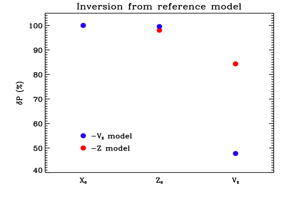
Figure 2.: The parameter changes $\delta$P needed to make to P₀ to correctly fit the new observations. These new observations were generated using a model with a lower $Z_{0}$ (red) and a lower $V_{Z}$ (blue).

2.2. Recovery of original parameters

The final uncertainties may be sufficiently low that the observations do contain enough information to be able to distinguish safely between initial metal mass fraction $Z_{0}$ and diffusion of this $V_{Z}$ (our original scientific question). Assume that we have two new sets of observations, and that these O really come from a solar model with 1) lower $Z_{0}$ and 2) lower $V_{Z}$. If we use Eq. 1 to fit the new O (separately) while using the reference set of parameters as P₀ (the initial guess), we will obtain non-zero negative values of $\delta Z_{0}$ and $\delta V_{Z}$ respectively, only if the observations contain sufficient information. If there is not enough information contained in the observations, then $\delta Z_{0}\sim\delta V_{Z}\sim 0$.

Figure 2 shows the values of $\delta$P (relative to the original value of P, for scaling purposes) for some of the parameters of the models, when attempting to fit a set of observations generated from a model with a reduced $Z_{0}$ (red) and a reduced $V_{Z}$ (blue). As the figure shows, some non-zero $\delta$P are needed to account for the new observations.

• When inverting using the lower $Z_{0}$ model observations (red), $\delta Z_{0}$ is negative. This means that we need to reduce the original $Z_{0}$ value to a lower one — consistent with the input model. However, we also see a negative contribution to $V_{Z}$; ideally $V_{Z}$ would not change, because it was not changed in this model, just as $X_{0}$ does not change.

• When inverting using the lower $V_{Z}$ model observations (blue), we obtain a much more negative $\delta V_{Z}$ (but no change in $Z_{0}$), indicating a necessary downward revision of only $V_{Z}$ — consistent with the input model.

These results are preliminary, but encouraging: there is some indication in the set of observables that we may be able to distinguish between initial metal abundance and diffusion of this using abundance measurements and seismic data.

Acknowledgments.

OLC wishes to acknowledge David Salabert for help with MATLAB. RAG is very grateful to the IAC for its visitor support. SM wishes to thank Sébastien Couvidat for his help with Fortran. This research was in part supported by the European Helio- and Asteroseismology Network (HELAS), a major international collaboration funded by the European Commission’s Sixth Framework Programme and by the CNES/GOLF grant at SAp, CEA, Saclay.

References

- Christensen-Dalsgaard (2007) Christensen-Dalsgaard, J. 2007, arXiv:0710.3106
- Creevey (2008) Creevey 2008, arXiv:0810.2191
- Creevey (2009) Creevey, 2009, this proceedings (arXiv:0810.2442)
- Grevesse & Noels (1993) Grevesse & Noels, 1993, Origin and evolution of the elements
- Mathur et al. (2007) Mathur, S., Turck-Chièze, S., Couvidat, S. & García, R.A. 2007, ApJ, 668, 594
- Morel (1997) Morel, 1997, A&AS, 124, 597