Multirate integration of axisymmetric step-flow equations

Abstract

We present a multirate method that is particularly suited for integrating the systems of Ordinary Differential Equations (ODEs) that arise in step models of surface evolution. The surface of a crystal lattice, that is slightly miscut from a plane of symmetry, consists of a series of terraces separated by steps. Under the assumption of axisymmetry, the step radii satisfy a system of ODEs that reflects the steps’ response to step line tension and step-step interactions. Two main problems arise in the numerical solution of these equations. First, the trajectory of the innermost step can become singular, resulting in a divergent step velocity. Second, when a step bunching instability arises, the motion of steps within a bunch becomes very strongly stable, resulting in “local stiffness”. The multirate method introduced in this paper ensures that small time steps are taken for singular and locally stiff components, while larger time steps are taken for the remaining ones. Special consideration is given to the construction of high order interpolants during run time which ensures fourth order accuracy of scheme for components of the solution sufficiently far away from singular trajectories.

1 Introduction.

In this paper, we present a multirate method that is suited for integrating systems of Ordinary Differential Equations (ODEs) which arise from step models describing nanostructure evolution. The strength of our method, in comparison to other existing multirate schemes, is its order of accuracy: our method is fourth order provided solutions are sufficiently smooth. A multirate method is basically one that takes different step sizes for different components of the solution [1]. When might such a need for different time steps arise? One situation where multirate methods may be more efficient than single rate ones is when a few of the components contain time singularities or are locally stiff. In this case, (explicit) single rate methods are likely to use small time steps for all the components, whereas a multirate one uses small time steps just for singular/locally stiff ones. We believe that this strategy significantly improves the efficiency of solution. Integration by our multirate method occurs in two stages. We first use an “outer” integrator to handle the non-singular/ non-stiff components and then an “inner” integrator to handle the singular/stiff ones. To perform the second inner integration, a small number of components from the outer solution must be interpolated. The high order of accuracy of the multirate scheme relies on the interpolation being of a sufficiently high order. One of our key results in this paper is that for a multirate method to be $n^{th}$ order, the interpolation must be $(n-1)^{st}$ order. We demonstrate our method by using a fourth order Runge-Kutta method (with error control) for the inner and outer schemes and coupling them together with cubic interpolants.

Multirate schemes were first studied by Gear and Wells [1]. Further treatments can be found in [2, 3, 4, 5, 6, 7, 8], and the references therein. However, considering the wide variety of methods which researchers have used to improve the performance and accuracy of integration codes, it is surprising to learn that multirate schemes have received only modest attention. This is even more surprising, given that algorithms using somewhat similar concepts are well developed for the numerical solution of PDEs — e.g. Adaptive Mesh Refinement (AMR) in the field of Hyperbolic PDEs [9, 10]. The applications of multirate methods seem mostly confined to $N$-body problems [4, 5], and equations arising from electrical networks [6, 7]. The work presented here is, as far as we are aware, the first instance of a multirate scheme applied to a problem in surface evolution.

Our method is fairly similar to the one described in [3], which is second order. For example: we first advance and interpolate the slow components, and then integrate the fast components — this is the “slowest first” paradigm described in [1]. We also automatically detect the fast components by looking at the error estimates produced using an embedded formula. The main differences are that: (i) our method is fourth order in time for sufficiently smooth solutions and (ii) our method is most effective when applied to the types of ODEs that commonly arise in models of step surface evolution. We will discuss (ii) in more detail later on in the paper, but for now we make the comment that a necessary but not sufficient condition for our method to work is that the ODE system be locally coupled. The strengths of our method are that automatic step size selection is simple to implement, and that there is a lower overhead cost because we do not have to interpolate all the slow components of the solution — this is one of the benefits of specializing to locally coupled systems.

The outline of this paper is as follows: in Section 2, we discuss why step models are studied and explain the physics behind the equations. In Section 3 we present the step equations, and in Section 4 we describe features of the equations that require special attention. In Section 5 we give the details of the numerical method and in particular, we discuss the important issue of interpolation in Section 5.3. We validate our code and present our results in Section 6 and summarize our findings with a conclusion in Section 7.

2 Physical Motivation.

The surface dynamics of crystal structures has received much recent attention [11, 12, 13] because of its relevance to the fabrication of nano-scale electronic devices, such as quantum dots [14]. Of interest to us here is the behavior of vicinal surfaces below the roughening temperature $T_{R}\/$. For any given material, a surface forming a small angle with a high symmetry plane of the crystal is called vicinal. The roughening temperature is the critical temperature below which steps become thermodynamically stable. Thus, a microscope image

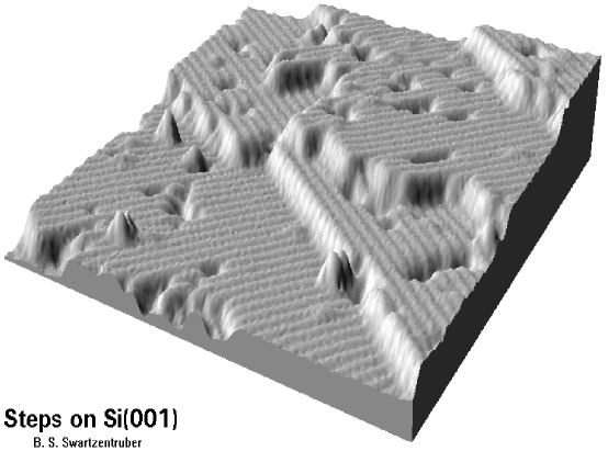
Figure 1: Image of a step on Silicon (001), taken with a Scanning Tunneling Microscope (courtesy of Brian Swartzentruber, Sandia National Laboratory).

of a surface below $T_{R}$, with a slight miscut angle, appears as made from a series of terraces separated by steps of atomic height — see Figure LABEL:fig:Silicon for an example in Silicon. As the surface evolves, the steps move and change their shape, but the steps are well defined and have a lifetime that is long enough to be directly observable. When the temperature is increased above $T_{R}$, a Kosterlitz-Thouless phase transition occurs [15], and the surface becomes statistically rough — as characterized by the divergence of the height–height correlation function [16, 17]. For many physical applications (such as epitaxy) the operating temperatures are below $T_{R}\/$, and this mesoscale description of a surface in terms of steps and their evolution is very useful. A step model can account for finite size effects occurring at the atomic scale, while remaining computationally simple — simulations with step models can be done over much longer time periods than, for example, with atomistic models of the surfaces.

The step’s shape can, in general, be very complicated. Thus, quantitative descriptions for how steps interact with one another can be very difficult to derive, and a complete description of an arbitrarily shaped nanostructure in terms of its steps is currently not available. As a result, theoretical studies have been restricted to simple nanostructure geometries and step shapes. The BCF model, proposed by Burton, Cabrera and Frank [18] in 1951, deals with a monotonic step train consisting of an infinite number of parallel steps — see Figure 2.

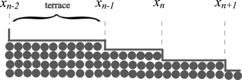
Figure 2: Sketch of the geometry in the Burton, Cabrera and Frank (BCF) 1-D step model. The step positions $x_{n}\/$ and the terraces are shown.

I

n this model, the steps edges are separated by atomically smooth terraces, and each step position is uniquely described by a single scalar quantity $x_{n}(t)\/$ — where the index $n\/$ labels the step. Using this model, Burton, Cabrera and Frank were able to describe the evolution of a (1 dimensional) stepped surface, under non-equilibrium conditions, in terms of its steps.

In 1988, Rettori and Villain [19] considered a 2D array of circular mounds, and incorporated the effects of step line tension into the BCF model. The nanostructures that they studied consist of a finite number of concentric circular layers, in a “wedding cake” configuration – see Figure 3. This step system can also be used to describe the “healing” of small circular pits [20] produced by scanning tunneling microscopes. The

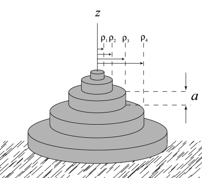
Figure 3: “Wedding Cake” step configuration for an axisymmetric nanostructure, with a finite number of concentric, circular steps. The step height $a$ is of the order of the crystal’s lattice constant. The number of steps considered in this paper is much larger than what is shown in this picture.

radius of each layer $\rho_{n}(t)\/$ is assumed to be a continuous function of time. Physical considerations then lead to a set of locally coupled ODEs for the radii. Similar sets of equations can be found in [21, 22, 23]. There are two main competing physical processes that take place on a stepped surface, in the absence of evaporation and desorption. The first one is the diffusion of adsorbed atoms (“adatoms”) across terraces, which is characterized by a diffusivity $D_{s}\/$. The second one is the attachment-detachment of adatoms at step edges, which is characterized by the kinetic coefficients $k_{+}\/$ and $k_{-}\/$ — see Figure 4. Experimental evidence [24] suggests that, for some materials, attachment from the terrace above requires overcoming a higher activation energy barrier than attachment from the terrace below, so that $k_{+}>k_{-}\/$. However, in this paper we consider only $k_{+}=k_{-}=k\/$, and disregard this (possible) asymmetry in the step attachment-detachment — known in the literature as an Ehrlich-Schwoebel (ES) Barrier [24, 25, 26]. Furthermore, we neglect the diffusion of adsorbed vacancies and the diffusion of adatoms along step edges [27].

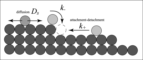
Figure 4: Sketch of the transport processes on a stepped surface, characterized by the attachment-detachment coefficients $k_{+}\/$ and $k_{-}\/$, and by the terrace diffusivity $D_{s}\/$. Throughout this paper, we take $k_{+}=k_{-}$.

3 Governing Equations.

In this section, we present the (non-dimensional) evolution equations for a finite axisymmetric nanostructure with ${\displaystyle N\geq 5\,}\/$ steps, relaxing in the absence of deposition and evaporation — see Figure 3. Derivations of these equations can be found in [21, 22].

Every step in the structure is subject to two physical effects that drive its motion. The first is a step-line tension, arising from a Gibbs-Thomson mechanism [28]. An isolated, circular step of radius $\rho(t)\/$, on top of an infinite substrate, initially devoid of adatoms, reduces its perimeter (and hence its radius) by emitting adatoms at a rate proportional to its curvature [11] — i.e. ${\displaystyle\dot{\rho}\propto-1/\rho}\/$. The second effect is a repulsive interaction with neighboring steps, characterized by a potential function that is inversely proportional to the square of the distance between the steps [29]. Steps in the bulk of the structure (with a smaller curvature) tend to be less affected by the step-line tension compared to steps near the top.

Let ${\displaystyle\rho_{n}=\rho_{n}(t)}\/$ ${\displaystyle(1\leq n\leq N)}\/$ be the positions of the steps — numbered starting from the top of the nanostructure. Thus ${\displaystyle 0<\rho_{1}<\rho_{2}\dots<\rho_{N}<\infty}\/$, with ${\displaystyle\rho_{1}}\/$ the radius of the innermost step and ${\displaystyle\rho_{N}}\/$ the radius of the outermost step. Define ${\displaystyle\Lambda_{n}}\/$, ${\displaystyle R_{n}}\/$, and ${\displaystyle\Delta_{n}}\/$, by:

$${\displaystyle\left.\begin{array}[]{lclcl}\Lambda_{1}&=&\lambda(\rho_{1},\rho_{2})\/,\\ \Lambda_{n}&=&\lambda(\rho_{n-1},\rho_{n})+\lambda(\rho_{n},\rho_{n+1})\/,\quad\mbox{for}\;\;2\leq n\leq N-1\/,\\ \Lambda_{N}&=&\lambda(\rho_{N-1},\rho_{N})\/,\end{array}\;\right\}}\/$$ (1)

$${\displaystyle\hskip 36.135pt\mbox{where}\quad\lambda(\rho_{i},\rho_{j})=\frac{2\,\rho_{i}}{\rho_{i}+\rho_{j}}\,\frac{1}{(\rho_{i}-\rho_{j})^{3}}+\frac{1}{\rho_{j}}\,\left(\frac{\rho_{i}}{\rho_{i}^{2}-\rho_{j}^{2}}\right)^{2}\,,}\/$$ (2)

$${\displaystyle\left.\begin{array}[]{lcl}R_{n}&=&{\displaystyle\frac{1}{\rho_{n}}}+\varepsilon\,\Lambda_{n}\/,\quad\mbox{for}\;\;1\leq n\leq N\/,\end{array}\right.}\/$$ (3)

$${\displaystyle\left.\begin{array}[]{lcl}\Delta_{n}&=&m_{1}\,\ln{\displaystyle\frac{\rho_{n+1}}{\rho_{n}}}+m_{2}\,\left({\displaystyle\frac{1}{\rho_{n+1}}+\frac{1}{\rho_{n}}}\right)\/,\quad\mbox{for}\;\;1\leq n\leq N-1\/,\end{array}\right.}\/$$ (4)

where ${\displaystyle\varepsilon}\/$, ${\displaystyle m_{1}}\/$, and ${\displaystyle m_{2}}\/$ (as well as ${\displaystyle\gamma}\/$ below) are non-dimensional constants. Then the step-flow equations are

$$\frac{d}{dt}\rho_{1} = \frac{\gamma}{\rho_{1}}\,\left(\frac{R_{2}-R_{1}}{\Delta_{1}}\right)\/,$$ (5)

$$\frac{d}{dt}\rho_{n} = \frac{\gamma}{\rho_{n}}\,\left(\frac{R_{n+1}-R_{n}}{\Delta_{n}}-\frac{R_{n}-R_{n-1}}{\Delta_{n-1}}\right)\/,\quad\mbox{for}\;\;2\leq n\leq N-1\/,$$ (6)

$$\frac{d}{dt}\rho_{N} = \frac{\gamma}{\rho_{N}}\,\left(-\frac{R_{N}-R_{N-1}}{\Delta_{N-1}}\right)\/.$$ (7)

The non-dimensional constants are as follows:

• The parameter ${\displaystyle\varepsilon>0}\/$ measures the strength of the step-step interactions relative to the strength of the step line tension. It is given by

  $$\varepsilon=\frac{2}{3}\,\frac{g_{3}}{g_{1}}\,\left(\frac{a}{L}\right)^{2}\/,$$

  where ${\displaystyle g_{3}}\/$ is the step-step interaction coefficient [29], ${\displaystyle g_{1}}\/$ is the step stiffness [11], ${\displaystyle a}\/$ is the height of a single step, and ${\displaystyle L}\/$ is a typical value for the radii – for example, it could be the initial radius of the final step in the structure. We note that, in many experimental situations, ${\displaystyle 0<\varepsilon\ll 1}\/$.

• The parameters ${\displaystyle 0\leq m_{1},m_{2}\leq 1}\/$ are given by

  $$m_{1}=\frac{k\,L}{k\,L+D_{s}}\quad\mbox{and}\quad m_{2}=\frac{D_{s}}{k\,L+D_{s}}\/,$$

  where ${\displaystyle k}\/$ is the adatom attachment-detachment coefficient at a step, and ${\displaystyle D_{s}}\/$ is the adatom terrace diffusivity. The ratio

  $$m=\frac{m_{2}}{m_{1}\,\Delta\rho}=\frac{D_{s}}{k\,L_{w}}\/,$$

  where ${\displaystyle\Delta\rho=\rho_{n+1}-\rho_{n}\,}\/$ and ${\displaystyle L_{w}\equiv L\Delta\rho}\/$ is a typical terrace width, measures the competition between diffusion and attachment-detachment — see equation (4).

• The dimensionless parameter ${\displaystyle\gamma}\/$ is given by

  $$\gamma=\left(\frac{g_{1}\Omega_{s}}{k_{B}T}\right)(\Omega_{s}c_{s})\left(\frac{a}{L}\right)\left(\frac{D_{s}}{LU}\right)\,m_{1}\/,$$

  where ${\displaystyle\Omega_{s}}\/$ is the atomic area, ${\displaystyle k_{B}}\/$ is the Boltzmann constant, ${\displaystyle T}\/$ is the absolute temperature, ${\displaystyle c_{s}}\/$ is the equilibrium density of adatoms at a straight, isolated, step and ${\displaystyle U}\/$ is a typical bulk step velocity.

We note that, of the physical parameters involved in the definitions of the non-dimensional constants above, some — such as the terrace diffusivity ${\displaystyle D_{s}}\/$, have been extensively tabulated [30], while others — such as ${\displaystyle c_{s}}\/$ and ${\displaystyle U}\/$, can be inferred from experiments [12, 31]. However, for the purposes of simulation, we can take ${\displaystyle m_{1}=m_{2}=\gamma=1/2}\/$ without loss of generality, by an appropriate rescaling of the step radii and time.

Equations (5) – (7) constitute a pentadiagonal system, of the form

$$\frac{d\rho_{n}}{dt}=F_{n}\left(\rho_{n-2}\/,\,\rho_{n-1}\/,\,\rho_{n}\/,\,\rho_{n+1}\/,\,\rho_{n+2}\right)\/,$$ (8)

where all the ${\displaystyle F_{n}}\/$ have the same functional form, with the exception of ${\displaystyle F_{1}}\/$, ${\displaystyle F_{2}}\/$, ${\displaystyle F_{N-1}}\/$, and ${\displaystyle F_{N}}\/$ — which govern the behavior of the first and final two steps. Notice that if ${\displaystyle F=F_{n}}\/$ denotes the common rate function for the bulk of the steps (${\displaystyle 2<n<N-2}\/$), then

$$F_{N-1}(\rho_{N-3}\/,\,\rho_{N-2}\/,\,\rho_{N-1}\/,\,\rho_{N}) = \lim_{\zeta\to\infty}F(\rho_{N-3}\/,\,\rho_{N-2}\/,\,\rho_{N-1}\/,\,\rho_{N}\/,\,\zeta)\/,$$

$$F_{N}(\rho_{N-2}\/,\,\rho_{N-1}\/,\,\rho_{N}) = \lim_{\eta\to\infty}\lim_{\zeta\to\infty}F(\rho_{N-2}\/,\,\rho_{N-1}\/,\,\rho_{N}\/,\,\eta\/,\,\zeta)\/.$$

In this paper, we present a multirate method for integrating the equations (5) – (7), when ${\displaystyle\varepsilon\ll 1}\/$. However, we believe that the method presented here should be applicable to general sets of locally coupled ODEs, which are locally stiff (see Section 4.2). In fact, our multirate method was designed to specifically tackle this problem.

4 Properties of The Step-Flow Equations.

Let us now turn our attention to the difficulties that arise when solving equations (5) – (7) numerically. The axisymmetric step-flow equations possess a number of peculiar properties which pose problems for standard integrators – hence the need for a multirate algorithm. For example, the singular collapse of the innermost step and stiffness, localized to only a few of the components, are two (different) situations under which a standard integrator is forced to use small time steps. In these cases, a single rate method uses small time steps for all components. In contrast, a multirate method will use small time steps only when it has to, so that most of the components are integrated with a large time step. This strategy improves the efficiency of the integration.

The singular collapse of the innermost step causes a loss in accuracy for most high order integrators near the point of collapse. Hence, we implement a low-order Simple Euler routine for the innermost step and its neighbors. Away from the singular step, we implement a fourth order multirate method with error control, which is able to efficiently integrate locally stiff components.

4.1 Singular Collapse of Steps.

Equations (5) – (7) have the property that ${\displaystyle\rho_{1}\rightarrow 0}\/$ in a finite time. The top step always undergoes a monotonic collapse because its radius always decreases under the effect of step-line tension. As the top step shrinks, it emits adatoms, causing the radii of the second and subsequent steps to grow as these are absorbed. When the top step completely disappears, the number of layers in the structure is reduced by one. As a result of the sequential collapse of top steps, a macroscopically flat region called a facet forms and grows on the top of the structure. Provided that the collapse of the top steps is tracked accurately, and the topmost ${\displaystyle\rho_{i}}\/$ is removed at each collapse, the growth of the facet is automatically accounted for.

When the first collapse occurs, $\rho_{2}$, $R_{3}$, $R_{2}$ and $\Delta_{2}$ replace $\rho_{1}$, $R_{2}$, $R_{1}$ and $\Delta_{1}$ in (5), and (6) applies when $3\leq n\leq N-1$. A similar replacement occurs for the second and subsequent collapses. In this way, a given index tracks always the same step throughout the integration.

Let ${\displaystyle\tau_{1}}\/$ be the collapse time for ${\displaystyle\rho_{1}}\/$. Then it can be shown [32] that as $t\rightarrow\tau_{1}$,

$$\rho_{1}\sim C_{1}(\tau_{1}-t)^{1/2}+C_{2}(\tau_{1}-t)\,\ln(\tau_{1}-t)+O(\tau_{1}-t)\/.$$ (9)

For some constants $C_{1}$ and $C_{2}$. The square root behavior in (9) comes from the fact that the leading order behavior for $\rho_{1}\ll 1$ in equation (5) stems from a line tension: $\dot{\rho}_{1}\sim 1/\rho_{1}$. Thus the derivatives of ${\displaystyle\rho_{1}}\/$ are divergent at the time of collapse. Since (5) – (7) is a locally coupled set of equations, we also expect $\rho_{i}$, for $2<i\ll N$, to be singular but for the solutions to become more regular near $\tau_{1}$ as $i$ becomes larger. Since the accuracy of high order integrators usually relies on the solution having enough bounded derivatives, this means that standard high order solvers will lose accuracy near the time of collapse. For example, consider a method with truncation error ${\displaystyle O((\Delta t)^{p}\,y^{(p)})}\/$ for smooth solutions ${\displaystyle y=y(t)}\/$, and time step ${\displaystyle\Delta t}\/$. Let ${\displaystyle t}\/$ be a time ${\displaystyle m}\/$ steps away from $\tau_{1}$, so that ${\displaystyle\tau_{1}-t=m\,\Delta t}\/$. Then, given the square root singularity in (9), the error near $\tau_{1}$ will be increased to

$$\mbox{error}=O(m^{-p+1/2}(\Delta t)^{1/2})\/.$$ (10)

Furthermore, consider the issue of automatic time step selection in an adaptive integration code. This is usually done by estimating the local truncation error, and updating the time step size with a formula for the truncation error that assumes a smooth solution. For example, consider a Runge-Kutta scheme using an embedded higher order formula to estimate the local truncation error. Such an algorithm updates the time step size using a formula like [33]

$$\Delta t_{\textrm{new}}=\Delta t_{\textrm{old}}\,\left(\frac{\textrm{desired error}}{\textrm{estimated error}}\right)^{\displaystyle\frac{1}{1+\alpha}}\/,$$ (11)

where ${\displaystyle\alpha}\/$ is the order of the integrator. Equation (11) is invalid near a time singularity, because from (10), the error near $\tau_{1}$ does not scale as ${\displaystyle\Delta t^{\alpha+1}}\/$. The resulting behavior is somewhat unpredictable: an adaptive integrator may take a very large number of tiny steps – rendering it very inefficient – or it may simply abort, stating that the specified error tolerance is not achievable.

4.2 Local Stiffness

The aim of this subsection is to attempt to quantify the classes of systems for which the approach in this paper is effective. Before explaining what we mean by local stiffness, we first introduce some notation. For $i=1,2,...,N$, let $\rho_{i}(t)$ be the solution of the ODE system for some initial condition $\rho_{i}(0)$. For some integer $p$, let $\tilde{\rho}_{i}(t)$ be the solution with initial condition $\rho_{i}(0)+\nu\delta_{p,i}$, where ${\displaystyle\delta_{p\/,i}}\/$ is the Kronecker delta, and ${\displaystyle\nu}\/$ is small. Finally, let $\rho(t)\equiv(\rho_{1}(t),\rho_{2}(t),...,\rho_{N}(t))$ and $\tilde{\rho}(t)\equiv(\tilde{\rho}_{1}(t),\tilde{\rho}_{2}(t),...,\tilde{\rho}_{N}(t))$. We say that the $p^{th}$ component of the ODE system is strongly local if (i) the system is locally coupled and (ii) given any $\epsilon>0$, for all $t$, there exists an integer $d$ independent of $t$ such that for $|n-p|>d$, $|\tilde{\rho}_{n}(t)-\rho_{n}(t)|<\epsilon$. If every component is strongly local, we say that the ODE system is strongly local. Therefore, a system is strongly local if a small perturbation to any one of its components remains localized in component number.

Now we explain local stiffness. Recall that an ODE is stiff when the ratio of the slowest and fastest time scales is much greater than one. The simplest example of this is a situation where the solution of interest is strongly stable, so that small perturbations decay very rapidly, relative to the principal time scale of evolution. Now consider again the perturbation described in the previous paragraph. We say that the $p^{th}$ component of an ODE system is locally stiff if (i) it is strongly local and (ii) $||\tilde{\rho}(t)-\rho(t)||\rightarrow 0$ rapidly in time, relative to the principal time scale of evolution. Hence, the $p^{th}$ component of the solution is locally stiff if a perturbation to it remains localized in component number and decays rapidly in time. If every component is locally stiff, the the solution is globally stiff.

Once strong locality has been established in an ODE system, individual solution components can be designated as either being (locally) stiff or non-stiff. For the rest of this paper, when we refer to “stiff components” of the solution, we mean that the components are locally stiff. A “non-stiff component” is one that evolves on a time scale comparable to the principal time scale. With this in mind, we can design multirate strategies that handle stiff and non-stiff components separately. For example, we expect to be able to integrate all non-stiff components with large time steps using explicit solvers. If the number of stiff components is relatively small, we can use the same explicit method on the stiff components also, but with much smaller time steps because of stability constraints. If on the other hand the number of stiff components is fairly large, we should resort to a fully implicit stiff solver.

At this point it is worth comparing our approach with other work in the literature dealing with problems involving disparate time scales. Gear and Kevrikidis [34] propose their “projective integration” method to deal with situations where there is a gap in the spectrum of time scales: the main evolution of a (stable) solution occurs slowly, with perturbations decaying much more quickly. For a linear problem, this corresponds to a situation where the eigenvalues can be separated into two groups: one set of moderate sized eigenvalues, and another set with large negative real parts. Projective integration requires two ODE solvers: an “inner” and an “outer” integrator. The idea is to take many small steps using the inner solver — so that the fast modes are damped out, followed by a large projective step with the outer integrator. The process is then repeated. This method (which is not multirate) is well-suited to handling problems where many, or all, of the solution components are rapidly attracted to a slowly varying manifold. Note that there is no notion of “locality” in this approach: the fast modes can potentially be coupled with all the slow ones.

Our multirate method also involves an “inner” and an “outer” integrator. As discussed above, the property of local stiffness means that a certain subset of the solution components have much stronger stability than the others. These stiff components are handled by an “inner” integrator while the non-stiff ones are taken care of using an “outer” solver. However, in contrast to the work of Gear and Kevrikidis, our method is more suited to systems where a small fraction of the components is stiff at any time during the integration. In fact, in terms of the ODE’s evolution in time, one can think of projective integration as using the inner/outer integrators in “series”, whereas our multirate method uses them in “parallel”.

4.3 Local stiffness for the step flow equations.

We will now show that $\rho_{n}$, the radius of a bulk step, in (6) is strongly local provided $1\ll n\ll N$ and hence, away from the facet and the substrate, any stiffness that arises is localized. For a bulk step, the physical origin of the rapid decay comes from the nature of step interactions in equation (2). Steps strongly repel each other when they get too close together. Consider a configuration where some of the steps in the bulk are tightly bunched together, and most of the other steps are widely spaced apart. In this case, a step strictly (two steps away, at least, from the edge) inside a bunch is strongly stable, and hence stiff, because small perturbations in its trajectory are opposed by strong interactions from the neighboring steps. On the other hand, widely spaced steps do not experience such large forces, and respond to perturbations on much slower time scales. It turns out that these “step bunching” configurations are quite common in practice and are produced by the natural time evolution of the system. In fact, the step bunching instability [21, 35, 36] is a well-studied phenomenon in epitaxial growth, with applications in quantum dot technology [14] and nanolithography [37].

To analyze the decay of solutions, the direct approach would be to compute the Jacobian matrix and analyze its eigenspectrum. Unfortunately, while the Jacobian for the system in (5) – (7) can be computed analytically by linearizing at any fixed set of radii ${\displaystyle(\rho_{1},\,\rho_{2},\,...,\,\rho_{N-1},\,\rho_{N})}\/$, the expressions involved are very complicated, and do not give much insight as to why the equations should be stiff. Instead, we present below a less rigorous calculation, which allows us to relate the degree of local stiffness to the step spacing. Our approach is based on the fact that the number of equations, $N$, is generally rather large, and that the solutions of interest have a step spacing that is, piecewise, nearly constant. By this we mean that the step spacing ${\displaystyle\;\rho_{n+1}-\rho_{n}\;}\/$ changes slowly with ${\displaystyle n}\/$, except for a few places where it may change abruptly — the effect of these changes is much harder to analyze, and our method of attack ignores them since it is only valid far away from these rapid transition regions. However, the results of our numerical calculations indicate that their presence does not invalidate our analysis.

We begin by considering a configuration of steps which has a nearly constant step spacing, and expand the solution in the form $\,\rho_{n}=\rho_{0}+(n-1)\,\delta\,$ + $\delta^{2}\,v_{n}(t)+\dots\,$, where ${\displaystyle\rho_{0}=O(1)}\/$ is a constant, ${\displaystyle\delta}\/$ is the (constant) leading order step spacing and $\rho_{0}\gg(n-1)\,\delta\gg\delta^{2}\,v_{n}$. Substituting this expression into the step flow equations, and ignoring the equations for the boundary steps (corresponding to ${\displaystyle n=1\/,\,2\/,N-1\/,}\/$ and ${\displaystyle N}\/$), results in the following leading order equation for the perturbation $v_{n}$

$$\frac{dv_{n}}{dt}\,=-\frac{3\,\varepsilon}{2\,\delta^{4}}\,\left(v_{n-2}-4v_{n-1}+6v_{n}-4v_{n+1}+v_{n+2}\right)=-\frac{3\,\varepsilon}{2\,\delta^{4}}\,\left(\Delta^{2}\;v\right)_{n}\/,$$ (12)

where ${\displaystyle\Delta}\/$ is the discrete Laplacian: ${\displaystyle(\Delta\;v)_{n}=v_{n+1}-2\,v_{n}+v_{n-1}}\/$. To show that equation (12) has the property of strong locality, we consider the solution to the problem with the initial condition ${\displaystyle v_{n}(0)=\nu\delta_{n\/,\,p}}\/$, given by

$$v_{n}=\frac{\nu}{2\,\pi}\int_{-\pi}^{\pi}\,e^{i\,k\,(n-p)-\sigma(k)\,t}\,dk\/,\quad\quad\mbox{where}\quad\sigma(k)=\frac{24\,\varepsilon}{\delta^{4}}\,\sin^{4}\frac{k}{2},$$ (13)

with $\nu\ll 1$. When $|n-p|\gg 1$, $v_{n}\rightarrow 0$ exponentially because the integrand in (13) is $2\pi$-periodic. Hence the delta function initial condition remains localized for all $t$.

Also, note that equation (12) has free normal modes given by

$$v_{n}=e^{i\,k\,n-\sigma(k)\,t}\/,$$ (14)

and ${\displaystyle-\pi<k\leq\pi}\/$ is the wave-number. It follows that the time scales behave like the fourth power of the step spacing. Hence, widely spaced steps evolve on a slow time scale whereas step bunches, which consist of sets of tightly packed steps, give rise to fast time scales and local stiffness.

5 Algorithm Details.

5.1 Algorithm Overview

The goal of our method is to efficiently solve a system of locally coupled ODEs where only a few of the components are stiff. A standard explicit integrator would take small time steps for all components of the solution. In contrast, our multirate method takes large steps for the non-stiff components, and small steps for the stiff ones.

The algorithm starts by taking an explicit, global time step, say: from $t_{n}\/$ to $t_{n+1}\/$. An embedded formula is then used to obtain an estimate of the Local Truncation Error (LTE) for each component of the solution. In general, some of the LTEs will be unacceptably large (because the associated solution components are stiff), while others will have acceptable sizes. The algorithm checks if the components with acceptable LTEs satisfy the preset tolerance levels. If they do not, the step size is reduced and another global time step is attempted. If they do, a second round of integration is performed to correct the components with large LTEs. Hence, the algorithm is as follows:

Algorithm 5.1

• Take a step from $t_{n}$ to $t_{n+1}$.

• Let ${\displaystyle e_{i}}\/$ be the LTE for the ${\displaystyle i}\/$-th component, let ${\displaystyle\mu}\/$ be the $P^{th}$ percentile of all the LTEs, and let ${\displaystyle tol_{i}}\/$ be the required error tolerance for $i$-th component. For example, if $P=10$, then $90\%$ of the errors are larger than $\mu$. If $P=50$, $\mu$ is the median.

• For some real number ${\displaystyle k}\/$, flag all the components whose LTEs are greater than ${\displaystyle 10^{k}\mu}\/$ (our code uses ${\displaystyle k=2}\/$) as being possibly stiff.

• Check if the unflagged solution components satisfy the tolerance requirements, i.e. $M\equiv Max(|e_{i}/tol_{i}|)<1$ where $Max()$ is taken over all unflagged components only.

• • If they do, the step is successful. The step size is increased using the formula (11) with $M^{-1}>1$ as the ratio of errors.

  • Perform a second integration to correct the flagged components (see Figure 5).

  • Increase the step size according to formula (11). Increase $n$ and go back to step 1.

• • If they do not, the step is not successful. Reduce the step size according to (11) with $M^{-1}<1$ as the ratio of errors.

  • Do not increase $n$ and go back to step 1.

The second integration is basically done only for the stiff components, and it involves many small sub-steps within the interval ${\displaystyle[t_{n},t_{n+1}]}\/$ to ensure stability. Although this second round of integration takes a large number of steps, it only needs to be done for a small subset of the solution components.

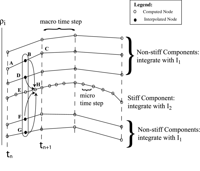
Figure 5: Schematic showing the two phases of integration with the time-steppers ${\displaystyle I_{1}}\/$ and ${\displaystyle I_{2}}\/$. Large time steps are taken using $I_{1}$ in the slowly varying bulk while smaller time steps are taken for stiff components using $I_{2}$. Here, point B is interpolated from points A and C, with D, F, and G obtained in a similar fashion. Because equations (5 – 7) are pentadiagonal, all the points B, D, E, F, and G are needed to to compute point H. Finally, we point out that in practice the stiff components are not isolated, but appear in bunches.

To perform the second integration, values for the non-stiff components at all times $t\in(t_{n},t_{n+1})$ along the boundaries of any stiff set of steps are needed — see Figure 5. For example, in the case of a pentadiagonal system, the values of two non-stiff components are needed on each side of a stiff region. One way to generate dense output from the non-stiff components, between ${\displaystyle t_{n}}\/$ and ${\displaystyle t_{n+1}}\/$, is through interpolation. In this paper we use cubic interpolatants which are generated by using the intermediate stage function evaluations in a Runge-Kutta method. In Section 5.3, we give more details on the construction of these interpolants and demonstrate that cubic interpolation is consistent with a multirate method that is globally fourth order.

Once solution components have been flagged as requiring re-integration, the local coupling means that some of the non-stiff components may also have to be re-integrated. Because (5) – (7) is a pentadiagonal system of equations, if only $r_{m}(t)$ and $r_{m+2}(t)$ are stiff components with large LTEs, then all three of the components $r_{m}(t),r_{m+1}(t)$ and $r_{m+2}(t)$ must be re-integrated as a set, using the dense output from $r_{m-2}(t)$, $r_{m-1}(t)$, $r_{m+3}(t)$ and $r_{m+4}(t)$ as ‘boundary conditions’. Hence, the algorithm is slightly wasteful in that although $r_{m+1}(t)$ was deemed accurate enough, it still had to be integrated for a second time.

Note that our algorithm uses the LTE in a different way from conventional embedded RK methods: Instead of immediately scaling the time step if the smallest LTE is greater than the tolerance level, we make a note of which components had the largest LTEs by analyzing their distribution: it might not be efficient to retake the time step for every component, if only a few of them are inaccurate. The largest LTEs (in the sense of being larger than $10^{k}\mu$ in Algorithm 5.1) are discarded, and then the time step scaled according to the largest of the remaining errors. Hence, we get a larger time step for a majority of the solution components, and the way that this time step is adjusted throughout the course of the integration is not affected by the presence of a few either rapidly varying or stiff components.

For the rest of this paper, we will call the first time stepper $I_{1}$ (used to generate the LTEs in the first place), and the second time stepper $I_{2}$ (used to re-integate stiff components with large LTEs). In general, $I_{1}$ and $I_{2}$ do not have to be the same method, or of the same order, but $I_{1}$ has to be able to generate estimates of the Local Truncation Error. In our code, $I_{1}$ is a Cash-Karp Runge-Kutta Formula [33] and $I_{2}$ depends on the solution component: if the re-integration involves the innermost step (see Section 5.2), we take $I_{2}$ to be a Simple-Euler routine which adjusts its step size by step doubling; otherwise $I_{2}=I_{1}$. In other words, there are two possibilities which can arise when performing the re-integration with $I_{2}$:

1. The re-integration involves solution components which include the innermost step. In the following analysis, we will assume this is $\rho_{1}$.

2. The re-integration does not involve the innermost step.

The reason to distinguish between these two cases is that (1) will involve integration of singular trajectories (see equation (9)), but in general, (2) will not. Using step doubling in (1) is a fairly crude way of adjusting the time step. However, resorting to an embedded formula is not possible when (11) breaks down, so using step doubling to monitor the quality of the solution is reasonable in this case.

5.2 Treatment of Singular Collapse of Top Step

From equation (9), we have seen that $\rho_{1}\rightarrow 0$ in a singular fashion, causing problems for standard high order integrators. Our treatment uses a Simple Euler method whenever the re-integration of $\rho_{1}$ and neighboring singular components is involved: this is “optimal” in the sense that Simple Euler produces results that have the same accuracy as higher order methods (due to the singular nature of $\rho_{1}$) but is computationally cheaper. Furthermore, we are able to extract the time of collapse, $t_{1}$, using linear interpolation, which is consistent with Simple Euler’s order of accuracy.

Our method involves solving for $\rho_{1}^{2},\rho_{2},...\rho_{N}$ instead of $\rho_{1},\rho_{2},...,\rho_{N}$. Note that from (9),

$$\rho_{1}^{2}(t)\sim C_{3}(\tau_{1}-t)+C_{4}(\tau_{1}-t)^{3/2}\ln(\tau_{1}-t)$$ (15)

as $t\rightarrow\tau_{1}$ (the collapse time) for some constants $C_{3}$ and $C_{4}$, which means that $\rho_{1}^{2}$ has exactly one derivative at $\tau_{1}$. Our main reason for solving for $\rho_{1}^{2}$, instead of $\rho_{1}$, is not to improve accuracy, but rather to enable the algorithm to ‘step through’ the singularity at $t=\tau_{1}$, and use linear interpolation to obtain $\tau_{1}$, the time of collapse of the innermost step.

Taking square roots to recover $\rho_{1}$ will will result in a drastic loss in accuracy near $\tau_{1}$. At time $t$ close to $\tau_{1}$, consider taking a time step of size $\Delta t$ with component $\rho_{1}^{2}$ using Simple Euler. Let $\rho^{2}_{\textrm{exact}}(t+\Delta t)$ be the result of taking this time step using a ‘perfect’ integrator, producing the exact solution at $t+\Delta t$, given $\rho_{1}^{2}(t)$. Then, since the truncation error in Simple Euler is $O\left(\Delta t^{2}\frac{d^{2}\rho_{1}^{2}}{dt^{2}}\right)=O(\Delta t^{3/2}\ln\Delta t)$ from (15), we have

$$|\rho_{1}^{2}(t+\Delta t)-\rho^{2}_{\textrm{exact}}(t+\Delta t)| = O(\Delta t^{3/2}\ln\Delta t),$$ (16)

$$\Rightarrow\rho_{1} = \rho_{\textrm{exact}}\left(1+\frac{O(\Delta t^{3/2}\ln\Delta t))}{\rho_{\textrm{exact}}^{2}}\right)^{1/2}.$$ (17)

Therefore, if $\rho^{2}_{\textrm{exact}}\gg O(\Delta t^{3/2}\ln\Delta t)$ ($t$ sufficiently far away from the singularity) then the LTE for $\rho_{1}$, $|\rho_{1}-\rho_{\textrm{exact}}|$, is $O(\Delta t^{3/2}\ln\Delta t)$. However, if $\rho^{2}_{\textrm{exact}}\ll O(\Delta t^{3/2}\ln\Delta t)$ ($t$ is very close to $t_{1}$), then the LTE for $\rho_{1}$ is $O(\Delta t^{3/4}(\ln\Delta t)^{1/2})$, which is not a big improvement over (10). Note that these estimates for the LTE are independent of the order of $I_{2}$. When $I_{2}$ has ‘overstepped’ $\tau_{1}$ resulting in $\rho_{1}^{2}(t_{m})>0$ and $\rho_{1}^{2}(t_{m+1})<0$ for times $t=t_{m},t_{m+1}\equiv t_{m}+\Delta t$ ($t_{m}<\tau_{1}<t_{m+1}$), we set

$$\tau_{1}\approx\frac{\rho_{1}^{2}(t_{m+1})t_{m+1}}{\rho_{1}^{2}(t_{m})-\rho_{1}^{2}(t_{m+1})}-\frac{\rho_{1}^{2}(t_{m+1})t_{m}}{\rho_{1}^{2}(t_{m})-\rho_{1}^{2}(t_{m+1})},$$ (18)

as an approximation to the collapse time. Once $\rho_{1}$ has collapsed at $\tau_{1}$, it is removed from the system (5) – (7), the number of equations drops by one, and $\rho_{2}^{2}(t)$ replaces $\rho_{1}^{2}(t)$ as the new top step.

5.3 Interpolation

The key to making our multirate method high order lies in the ability to generate dense output from the non-stiff components with high accuracy. One way to generate dense output is to use interpolation. For some integrators, such as Backward Differentiation Formulae (BDF), is it obvious how to derive an interpolant that is consistent in order with the underlying integrator – BDF use extrapolation to advance the solution in time. For other integrators, such as Runge-Kutta schemes, constructing the interpolant is less obvious and this is the focus of the section. Note that we need to generate interpolants during run time using only the function evaluations that have already been computed by the integrator within each time step. The extra constraint of generating the interpolants during run time adds a non-trivial complication to the “traditional” interpolation problem, which has been studied extensively [38, 39]. Having successfully integrated the non-stiff components from $t_{n}$ to $t_{n+1}$, we have the point values $y_{n},y_{n+1}$ and the derivative $y_{n}^{\prime}$ at our disposal to construct the interpolant between $t_{n}$ and $t_{n+1}$. We do not have information about the derivative $y_{n+1}^{\prime}$. However, because we are constructing these interpolants during run time, we are at liberty to use the intermediate function evalulations inherent in the application of Runge-Kutta: this is valuable information that is not usually available in the traditional interpolation problem.

We have seen that our method performs integration in two phases: first we integrate a large number of non-stiff components, then we integrate a small number of stiff ones. Ideally, we would like the two integrations to have the same order. This is only possible if the interpolation of the non-stiff components is of a sufficiently high order – otherwise large interpolation errors will contaminate the accuracy in the stiff components. In the following paragraphs, when we generate dense output between points $t$ and $t+\Delta t$, we define an interpolant to be order $m$ when the interpolation error is $O(\Delta t^{m+1})$.

Let us assume that our inner and outer solvers are both $n^{th}$ order. First of all, let us calculate $m$ in terms of $n$ if we want our method to be globally $n^{th}$ order. For simplicity, we assume in this calculation that the effects of round-off error are negligible. Consider the ODE system

$$\mathbf{y}^{\prime}=\mathbf{F}(\mathbf{y},t).$$ (19)

Let us assume that we have taken a macro step of size $\Delta t$ and advanced the non-stiff components $\mathbf{y}_{r}(t)$ successfully from time $t$ to $t+\Delta t$. Also assume that we have taken $N$ micro steps of size $\Delta t_{i}$, $i=1,2,...,N$, for the stiff components $\mathbf{y}_{s}(t)$ so that $\sum_{i=1}^{N}\Delta t_{i}=\Delta t$. After taking these $N$ steps, the total error in $\mathbf{y}_{s}(t)$ will be

$$O\left(\sum_{i=1}^{N}\Delta t_{i}^{n+1}\right)+O\left(\sum_{i=1}^{N}\Delta t_{i}\Delta t^{m+1}\right).$$ (20)

The first term is the sum of the Local Truncation Errors caused by taking $N$ steps each of size $\Delta t_{i}$. The second term is the sum of the interpolation errors: note that to advance $\mathbf{y}_{s}$, an evaluation of $\mathbf{F}$ in between $t$ and $t+\Delta t$, in general, is required for the non-stiff neighbours of $\mathbf{y}_{s}$ and this incurs an interpolation error of size $O(\Delta t^{m+1})$. Therefore the error in $\mathbf{y}_{s}^{\prime}$ is also $O(\Delta t^{m+1})$ and the error in $\mathbf{y}_{s}$ is $O(\Delta t_{i}\Delta t^{m+1})$. It is clear that (20) simplifies to

$$O\left(\Delta t^{n+1},\Delta t^{m+2}\right),$$ (21)

and so for our multirate method to be globally $n^{th}$ order, we require $m=n-1$ – that is, we can afford for the order of the interpolation to be one less than the order of the integrator. For example, if our integrator is fourth order ($n=4$), we need to be able to construct cubic interpolants during run time. If our integrator is second order, then linear interpolation should be sufficient – as observed in [3].

We will now illustrate how these interpolants are constructed by taking the classical 4th order (non-adaptive) Runge-Kutta formula as an example and applying it to the autonomous ODE system $y^{\prime}=f(y)$:

Table 1: Coefficients in classical RK4

$a_{1}=0$	$b_{11}=0$
$a_{2}=\frac{1}{2}$	$b_{21}=\frac{1}{2}$	$b_{22}=0$
$a_{3}=\frac{1}{2}$	$b_{31}=0$	$b_{32}=\frac{1}{2}$	$b_{33}=0$
$a_{4}=1$	$b_{41}=0$	$b_{42}=0$	$b_{43}=1$	$b_{44}=0$
	$c_{1}=\frac{1}{6}$	$c_{2}=\frac{1}{3}$	$c_{3}=\frac{1}{3}$	$c_{4}=\frac{1}{6}$

The solution $y_{n}$ is advanced to $y_{n+1}$ through

$$y_{n+1}=y_{n}+\sum_{i=1}^{4}c_{i}k_{i},$$ (22)

where

$$k_{i}=\Delta tf(y_{n}+\sum_{j=1}^{i-1}b_{ij}k_{j}),$$ (23)

for $i=1,2,3,4$. It is easy to show that equation (22) implies that

$$y_{n+1}=y_{n}+\Delta ty_{n}^{\prime}+\frac{\Delta t^{2}}{2}y_{n}^{\prime\prime}+\frac{\Delta t^{3}}{3!}y_{n}^{\prime\prime\prime}+\frac{\Delta t^{4}}{4!}y_{n}^{(4)}+O(\Delta t^{5}).$$ (24)

Let us try to construct a quartic interpolant. Equation (24) motivates us to write this in the form

$$y(\chi\Delta t)=y_{n}+(\chi\Delta t)y_{n}^{\prime}+\frac{(\chi\Delta t)^{2}}{2}y_{n}^{\prime\prime}+\frac{(\chi\Delta t)^{3}}{3!}y_{n}^{\prime\prime\prime}+\frac{(\chi\Delta t)^{4}}{4!}y_{n}^{(4)}+O(\Delta t^{5}),$$ (25)

where $0\leq\chi\leq 1$. The problem is now to evaluate the derivatives $y_{n}^{(m)}$ in terms of the intermediate stage function evaluations $k_{i}$. This is done by (i) noting that

$$\begin{array}[]{lll}y_{n}^{\prime}&=&f_{n}\\ y_{n}^{\prime\prime}&=&f_{n}^{\prime}f_{n}\\ y_{n}^{\prime\prime\prime}&=&f_{n}{f_{n}^{\prime}}^{2}+f_{n}^{2}f_{n}^{\prime\prime}\\ y_{n}^{(4)}&=&f_{n}{f_{n}^{\prime}}^{3}+4f_{n}^{2}f_{n}^{\prime}f_{n}^{\prime\prime}+f_{n}^{3}f_{n}^{\prime\prime\prime}\end{array}$$ (26)

where $f_{n}\equiv f(y_{n})$ and similarly with $f_{n}^{\prime},f_{n}^{\prime\prime},...$, and (ii) expanding $k_{i}$ in Taylor series:

$$\begin{array}[]{lll}k_{1}&=&\Delta tf_{n},\\ k_{2}&=&\Delta tf_{n}+\frac{\Delta t^{2}}{2}f_{n}^{\prime}f_{n}+\frac{\Delta t^{3}}{8}f_{n}^{2}f_{n}^{\prime\prime}+\frac{\Delta t^{4}}{48}f_{n}^{3}f_{n}^{\prime\prime\prime}+O(\Delta t^{5}),\\ k_{3}&=&\Delta tf_{n}+\frac{\Delta t^{2}}{2}f_{n}^{\prime}f_{n}+\frac{\Delta t^{3}}{8}(2f_{n}{f_{n}^{\prime}}^{2}+f_{n}^{2}f_{n}^{\prime\prime})\\ &&+\frac{\Delta t^{4}}{48}(9f_{n}^{2}f_{n}^{\prime}f_{n}^{\prime\prime}+f_{n}^{3}f_{n}^{\prime\prime\prime})+O(\Delta t^{5}),\\ k_{4}&=&\Delta tf_{n}+\Delta t^{2}f_{n}^{\prime}f_{n}+\frac{\Delta t^{3}}{2}(f_{n}{f_{n}^{\prime}}^{2}+f_{n}^{2}f_{n}^{\prime\prime})\\ &&+\frac{\Delta t^{4}}{24}(6f_{n}f_{n}^{\prime 3}+15f_{n}^{2}f_{n}^{\prime}f_{n}^{\prime\prime}+4f_{n}^{3}f_{n}^{\prime\prime\prime})+O(\Delta t^{5}).\end{array}$$ (27)

A natural way to compute the $y_{n}^{(m)}$ would be to find the 7 terms $f_{n}$, $f_{n}^{\prime}f_{n}$, $f_{n}{f_{n}^{\prime}}^{2}$, $f_{n}^{2}f_{n}^{\prime\prime}$, $f_{n}{f_{n}^{\prime}}^{3}$, $f_{n}^{2}f_{n}^{\prime}f_{n}^{\prime\prime}$ and $f_{n}^{3}f_{n}^{\prime\prime\prime}$ in terms of the $k_{i}$ from (27) and then use them in (26). However, this is not possible because (27) becomes a system of 4 linear equations in 7 unknowns. We must therefore be a little less ambitious. In light of our previous comments on interpolation, we seek a cubic interpolant in the form

$$y(\chi\Delta t)=y_{n}+(\chi\Delta t)y_{n}^{\prime}+\frac{(\chi\Delta t)^{2}}{2}y_{n}^{\prime\prime}+\frac{(\chi\Delta t)^{3}}{3!}y_{n}^{\prime\prime\prime}+O(\Delta t^{4}).$$ (28)

Since we do not need the $y_{n}^{(4)}$ term, constructing $y_{n}^{\prime},y_{n}^{\prime\prime}$ and $y_{n}^{\prime\prime\prime}$ now requires only $f_{n}$, $f_{n}^{\prime}f_{n}$, $f_{n}{f_{n}^{\prime}}^{2}$ and $f_{n}^{2}f_{n}^{\prime\prime}$. Ignoring the $O(\Delta t^{4})$ terms, (27) constitutes 4 equations in 4 unknowns. Solving in terms of the $k_{i}$ yields

$$f_{n} = \frac{k_{1}}{\Delta t},$$ (29)

$$f_{n}f_{n}^{\prime} = \frac{1}{\Delta t^{2}}\left(-3k_{1}+2k_{2}+2k_{3}-k_{4}\right),$$ (30)

$$f_{n}^{2}f_{n}^{\prime\prime} = \frac{1}{\Delta t^{3}}\left(4k_{1}-8k_{3}+4k_{4}\right),$$ (31)

$$f_{n}{f_{n}^{\prime}}^{2} = \frac{1}{\Delta t^{3}}\left(-4k_{2}+4k_{3}\right),$$ (32)

so that the cubic interpolant is

$$y(\chi\Delta t)=y_{n}+\chi k_{1}+\frac{\chi^{2}}{2}\left(-3k_{1}+2k_{2}+2k_{3}-k_{4}\right)+\frac{2\chi^{3}}{3}\left(k_{1}-k_{2}-k_{3}+k_{4}\right).$$ (33)

We now turn our attention to Embedded Runge-Kutta Methods. Let us focus on the Cash-Karp formula in [33] which has the tableau

Table 2: Coefficients in the Cash-Karp 4-5 formula

$0$	0
$\frac{1}{5}$	$\frac{1}{5}$	0
$\frac{3}{10}$	$\frac{3}{40}$	$\frac{9}{40}$	0
$\frac{3}{5}$	$\frac{3}{10}$	$-\frac{9}{10}$	$\frac{6}{5}$	0
$1$	$-\frac{11}{54}$	$\frac{5}{2}$	$-\frac{70}{27}$	$\frac{35}{27}$	0
$\frac{7}{8}$	$\frac{1631}{55296}$	$\frac{175}{512}$	$\frac{575}{13824}$	$\frac{44275}{110592}$	$\frac{253}{4096}$	0
	$\frac{2825}{27648}$	$0$	$\frac{18575}{48384}$	$\frac{13525}{55296}$	$\frac{277}{14336}$	$\frac{1}{4}$
	$\frac{37}{378}$	$0$	$\frac{250}{621}$	$\frac{125}{594}$	$0$	$\frac{512}{1771}$

The analogue to (27) is

$$\begin{array}[]{lll}k_{1}&=&\Delta tf_{n},\\ k_{2}&=&\Delta tf_{n}+\frac{\Delta t^{2}}{5}f_{n}^{\prime}f_{n}+\frac{\Delta t^{3}}{50}f_{n}^{2}f_{n}^{\prime\prime}+\frac{\Delta t^{4}}{750}f_{n}^{3}f_{n}^{\prime\prime\prime}+O(\Delta t^{5}),\\ k_{3}&=&\Delta tf_{n}+\frac{3\Delta t^{2}}{10}f_{n}^{\prime}f_{n}+\frac{9\Delta t^{3}}{200}(f_{n}{f_{n}^{\prime}}^{2}+f_{n}^{2}f_{n}^{\prime\prime})\\ &&+\frac{9\Delta t^{4}}{2000}(4f_{n}^{2}f_{n}^{\prime}f_{n}^{\prime\prime}+f_{n}^{3}f_{n}^{\prime\prime\prime})+O(\Delta t^{5}),\\ k_{4}&=&\Delta tf_{n}+\frac{3\Delta t^{2}}{5}f_{n}^{\prime}f_{n}+\frac{9\Delta t^{3}}{50}(f_{n}{f_{n}^{\prime}}^{2}+f_{n}^{2}f_{n}^{\prime\prime})\\ &&+\frac{9\Delta t^{4}}{500}(3f_{n}f_{n}^{\prime 3}+8f_{n}^{2}f_{n}^{\prime}f_{n}^{\prime\prime}+2f_{n}^{3}f_{n}^{\prime\prime\prime})+O(\Delta t^{5}),\\ k_{5}&=&\Delta tf_{n}+\Delta t^{2}f_{n}^{\prime}f_{n}+\frac{\Delta t^{3}}{2}(f_{n}{f_{n}^{\prime}}^{2}+f_{n}^{2}f_{n}^{\prime\prime})\\ &&+\frac{\Delta t^{4}}{60}(7f_{n}f_{n}^{\prime 3}+40f_{n}^{2}f_{n}^{\prime}f_{n}^{\prime\prime}+10f_{n}^{3}f_{n}^{\prime\prime\prime})+O(\Delta t^{5}),\\ k_{6}&=&\Delta tf_{n}+\frac{7\Delta t^{2}}{8}f_{n}^{\prime}f_{n}+\frac{49\Delta t^{3}}{128}(f_{n}{f_{n}^{\prime}}^{2}+f_{n}^{2}f_{n}^{\prime\prime})\\ &&+\frac{7\Delta t^{4}}{3072}(46f_{n}f_{n}^{\prime 3}+196f_{n}^{2}f_{n}^{\prime}f_{n}^{\prime\prime}+49f_{n}^{3}f_{n}^{\prime\prime\prime})+O(\Delta t^{5}).\end{array}$$ (34)

Cash-Karp 4-5 is formally 4th order, so again, it is sufficient to interpolate with cubic polynomials. However, one would expect that since we have made two extra evaluations of $f(y)$, it would be possible to construct interpolants which have higher order. At first, this possibility seems promising. We note that in (34), with the exception of the $k_{2}$ equation, the terms $f_{n}^{2}f_{n}^{\prime}f_{n}^{\prime\prime}$ and $f_{n}^{3}f_{n}^{\prime\prime\prime}$ always appear together as $(4f_{n}^{2}f_{n}^{\prime}f_{n}^{\prime\prime}+f_{n}^{3}f_{n}^{\prime\prime\prime})$ and $f_{n}{f_{n}^{\prime}}^{2}$, $f_{n}^{2}f_{n}^{\prime\prime}$ always appear together as $(f_{n}{f_{n}^{\prime}}^{2}+f_{n}^{2}f_{n}^{\prime\prime})$. The equations for $k_{1},k_{3},k_{4},k_{5}$ and $k_{6}$ therefore give 5 equations in 5 unknowns, $f_{n}$, $f_{n}^{\prime}f_{n}$, $(f_{n}{f_{n}^{\prime}}^{2}+f_{n}^{2}f_{n}^{\prime\prime})$, $f_{n}f_{n}^{\prime 3}$ and $(4f_{n}^{2}f_{n}^{\prime}f_{n}^{\prime\prime}+f_{n}^{3}f_{n}^{\prime\prime\prime})$. Unfortunately, the matrix of the resulting linear system has a zero determinant and the equation

$$\begin{pmatrix}\begin{array}[]{lllll}\Delta t&0&0&0&0\\ \Delta t&\frac{3\Delta t^{2}}{10}&\frac{9\Delta t^{3}}{200}&0&\frac{9\Delta t^{4}}{2000}\\ \Delta t&\frac{3\Delta t^{2}}{5}&\frac{9\Delta t^{3}}{50}&\frac{27\Delta t^{4}}{500}&\frac{9\Delta t^{4}}{250}\\ \Delta t&\Delta t^{2}&\frac{\Delta t^{3}}{2}&\frac{7\Delta t^{4}}{60}&\frac{\Delta t^{4}}{6}\\ \Delta t&\frac{7\Delta t^{2}}{8}&\frac{49\Delta t^{3}}{128}&\frac{161\Delta t^{4}}{1536}&\frac{343\Delta t^{4}}{3072}\end{array}\end{pmatrix}\begin{pmatrix}\begin{array}[]{c}f_{n}\\ f_{n}^{\prime}f_{n}\\ f_{n}{f_{n}^{\prime}}^{2}+f_{n}^{2}f_{n}^{\prime\prime}\\ f_{n}{f_{n}^{\prime}}^{3}\\ 4f_{n}^{2}f_{n}^{\prime}f_{n}^{\prime\prime}+f_{n}^{3}f_{n}^{\prime\prime\prime}\end{array}\end{pmatrix}=\begin{pmatrix}\begin{array}[]{c}k_{1}\\ k_{3}\\ k_{4}\\ k_{5}\\ k_{6}\end{array}\end{pmatrix}$$ (35)

does not have a unique solution.

Going through the same process with Fehlberg’s pair does not improve the situation. It is not clear to us at this point whether the inability to build quartic interpolatants using the intermediate stage function evaluations is symptomatic of all RK45 pairs, or if it is possible to find Runge-Kutta families for which the equivalent of (35) is uniquely solvable. Although having quartic interpolants is not necessary for our multirate method to be globally fourth order, these interpolants – if they can be constructed – could be used to check the accuracy of the cubic interpolants in the same way that the fifth order RK formula is used to check the values predicted by the fourth order one. If the interpolation is deemed too inaccurate, the integration of the non-stiff components would have to be performed again using a smaller step size.

Construction of the cubic interpolant in Cash-Karp 45 is now fairly straightforward and we follow the same procedure as for classical RK4. There is now more than one possible cubic polynomial, depending on which $k_{i}$ to use in (34). Using the equations involving $k_{1}$, $k_{4}$ and $k_{5}$, we have

$$y(\chi\Delta t)=y_{n}+\chi k_{1}+\frac{\chi^{2}}{2}\left(-\frac{8}{3}k_{1}+\frac{25}{6}k_{4}-\frac{3}{2}k_{5}\right)+\frac{\chi^{3}}{6}\left(\frac{10}{3}k_{1}-\frac{25}{3}k_{4}+5k_{5}\right).$$ (36)

This is the interpolant used in our multirate code to generate the results in Section 6.

6 Validation and Results

Here we validate our code with different tests, each of which examines a particular aspect of the integration.

6.1 Validation

6.1.1 Collapse Times

To test the code’s ability to handle singular collapses, we used it to solve the (uncoupled) ODE system

$$\dot{r}_{i}=-1/r_{i}$$ (37)

for $i=1,2,...,N$ with initial condition $r_{i}(0)=i$.

The solution to this set of ODEs is $r_{i}(t)=\sqrt{i^{2}-2t}$. Note that the solution has the same leading order singular behaviour at the collapse times $t_{i}=i^{2}/2$ as equations (5)-(7). A second, more challenging, model problem is

$$\dot{r}_{i}=-1/r_{i}^{2},$$ (38)

with the same initial condition as before. The collapse times in this system take the form $t_{i}=i^{3}/3$ because the exact solutions are $r_{i}(t)=(i^{3}-3t)^{1/3}$: the solution near the collapse times in this case are even steeper than in (37). The results in Table LABEL:table1 show that our code is able to capture the collapse times to 4-5 significant digits of accuracy.

Table 3: First 5 collapse times for model systems (37) and (38). Both exact and numerical values are shown. The relative and absolute tolerances were $10^{-6}$ and $10^{-8}$ respectively.

Collapse time	eqn (37)	eqn (37)	eqn (38)	eqn (38)
	numerical	exact	numerical	exact
$t_{1}$	0.500000000	0.50	0.33334710950	0.333…
$t_{2}$	2.00002007041	2.00	2.66673866493	2.666…
$t_{3}$	4.50006868256	4.50	9.00020498167	9.000…
$t_{4}$	8.00013388581	8.00	21.33376504303	21.333…
$t_{5}$	12.5002133304	12.50	41.66743834183	41.666…

To test the accuracy of the collapse times generated from the full set of step flow equations (5) - (7), we used fixed step Simple Euler with $\Delta t=10^{-6}$ and linear interpolation to obtain a set of reference collapse times. Since this method of integration is computationally expensive, we initialized the simulation with only $N=15$ layers. These times were compared with data generated from the full multirate code with high order adaptive time stepping. The results are shown in Table 4.

Table 4: First five collapse times shown for a Diffusion Limited system (obtained by setting $m_{1}=1$, $m_{2}=0$ in equation (4) and $\gamma=1$ in (5)-(7)), with $\varepsilon=0.01$. The initial condition was a 15 layer profile with unit spacing.

Collapse time	Reference Solution	Multirate Solution
$t_{1}$	0.540289230794	0.540305641980
$t_{2}$	5.100219762927	5.100284674837
$t_{3}$	21.036583847637	21.036757035271
$t_{4}$	59.481455149416	59.481830949331
$t_{5}$	135.366866973862	135.367562952919

6.1.2 Convergence and error analysis

We used our multirate code to solve the simple wave equation $u_{t}+u_{x}=0$. By discretizing using the Method of Lines and one-sided (“upwind”) differences in space, we obtained $N$ coupled Ordinary Differential Equations which were solved using the initial condition $u(x,0)=e^{-(x+10)^{2}}$ and periodic boundary conditions. Unlike the axisymmetric step equations, this discretization of the wave equation does not have any time singularities and we expect fourth order convergence for every component. This is confirmed in Figure 6. Although $\Delta t$ and $\Delta t_{\textrm{micro}}$ constantly change because our algorithm uses adaptive step size control, we take $\Delta t\sim T/N$ as a measure of the average step size where $T$ is the final integration time. For the single rate method, $N$ is the number of steps and for the multirate method, $N$ is the total number of micro-steps. In the multirate code, a maximum macro-stepsize $\Delta t_{\textrm{macro}}=1$ was imposed, and all but the first and final macro-steps had size 1. The exact solution comes from solving the linear system of ODEs exactly using an eigenfunction expansion. As the integration progresses, the fraction of components that has to be reintegrated increases gradually as the solution broadens and its amplitude decreases: see Figure 7. A Matlab multirate code that produces the results in Figure 7 is given in the Appendix.

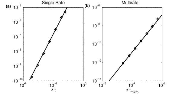
Figure 6: Fourth order convergence was obtained from solving a wave equation discretized using the method of lines. The domain was $-25\leq x\leq 25$ and $N=401$ equations were solved. The final integration time was $T=20$. Different (average) time step sizes were obtained by changing the tolerance level of the code. (a) Fourth order convergence of single rate Cash-Karp Runge Kutta. (b) Fourth order convergence of multirate Cash-Karp Runge-Kutta. The parameters used in Algorithm 5.1 were $k=-6$, $P=30$. The number of macrosteps used by the algorithm in every integration was 22.

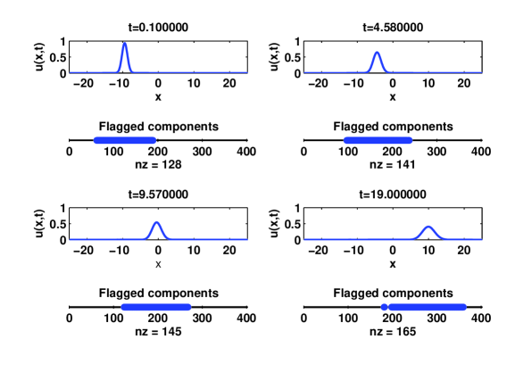
Figure 7: Solution of the advection equation, with unit wave speed, at different times, obtained using a multirate method. Components flagged as requiring a second integration are shown in each case; the number of such components is given by the variable $nz$. The total number of equations solved was $N=401$ and periodic boundary conditions were used on the domain $-25\leq x\leq 25$. Multirate parameters (described in Algorithm 5.1) were $k=-6$ and $P=30$.

6.2 Results

Figure 8(a) shows the results of an integration with $\varepsilon=10^{-3}$. Note that only those steps which are near the facet tend to pack closely together, but steps which are far away move relatively slowly and do not deviate significantly from their initial uniform configuration. This expanding front of closely packed steps represents the $t^{1/4}$ expansion of the facet radius [21, 22].

Figure 8(b) illustrates the separation in time scales of the solution components and shows which components of the solution are integrated for a second time. As expected, our algorithm takes large time steps for components which are far away from the facet. Near the facet and the collapsing top step, many relatively small steps are taken. For the rapidly varying components in this figure, only a representative sample of the meshpoints $t_{n}$ from the $I_{2}$ integration are shown.

In contrast, when $\varepsilon=10^{-5},10^{-6}$, steps can be closely packed even away from the facet. The plots in Figure 9 show that a step bunching instability arises when $\varepsilon$ is sufficiently small and are qualitatively very different to those in Figure 8. The instability originates from steps with smaller radii and gradually spreads outwards so that more and more steps bunch up. Our multirate scheme performs a second integration when bunching and local stiffness arise: therefore, our algorithm gradually becomes less efficient over time. However, as long as the fraction of bunched steps is not too large, our algorithm remains competitive compared to a standard adaptive 4th/5th order Runge-Kutta code. When the fraction of bunched steps becomes close to unity, the optimal strategy is to have the algorithm detect this automatically, and then switch to a fully implicit, single-rate stiff solver. We leave this as future work, noting that inversion of the pentadiagonal Jacobian only costs $O(N)$ operations (where $N$ is the total number of existing steps).

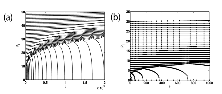
Figure 8: A step instability arises when $\varepsilon$ is sufficiently small. (a) Simulated relaxation of a nanostructure consisting of 200 steps, for a step train that is initially uniformly spaced. Only the first 50 steps are shown. (b) Results of a simulation with some of the time points of the multirate integration shown explicitly.

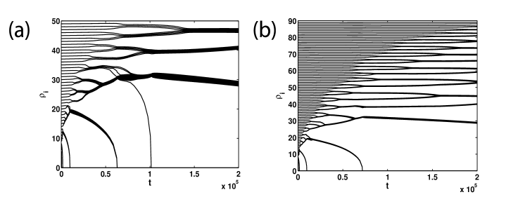
Figure 9: A step bunching instability arises when $\varepsilon$ is sufficiently small. (a) $\varepsilon=10^{-5}$. (b) $\varepsilon=10^{-6}$. Approximately the first 50 and 90 steps are shown respectively, out of 200.

7 Conclusions

In this paper, we present a multirate integration scheme that is designed to efficiently solve the systems of ODEs that arise in the relaxation of crystal mounds. These ODEs have two properties that call for a multirate strategy: the singular collapse of the innermost step and local stiffness. Our method automatically detects singular/stiff components in the solution and disregards them when computing the size of the bulk (macro) time step. The result is that the bulk timestep can be much larger than in a single rate method. The trade-off is a re-integration of the stiff components which usually consists of a small fraction of the total number of equations in the ODE system.

Our method is globally fourth order when applied to ODEs which have sufficiently smooth solutions – for example, the step equations studied in [23] and the wave equation discretized through the method of lines in Section 6.1.2. However, the time singularities present in the axisymmetric step-flow equations mean that near times of collapse, the integration of steps near the facet suffers a loss in accuracy. To specifically deal with the singular inner trajectories, our method couples a Simple Euler routine to the bulk solver. Given that the truncation error reduces to $O(\Delta t^{1/2})$ near the collapse time, independent of the method order, Simple Euler is the preferred method because it is computationally cheaper. Furthermore, the use of linear interpolation to extract collapse times is consistent with the method’s order.

The high order accuracy of our algorithm (when applied to bulk steps) relies on the ability to generate high order interpolants during the run-time of a one-step integration method. Our algorithm generates these interpolants by using the intermediate stage function evaluations of an embedded Runge-Kutta (RK) formula. Specifically, our method computes $3^{rd}$ order interpolants that are consistent with the $4^{th}$ order accuracy of the integrator. However, for general $n^{th}$ order RK formulae, we do not know if it is always possible to construct interpolants that have order $(n-1)$.

We see four main possible extensions to this work. The first is to generalize our multirate paradigm so that it can be used for (i) higher order Runge-Kutta formulae and (ii) multistep methods (e.g. BDF, Adams etc.) We believe that it should be possible to make any method multirate – the main obstacle in doing this is to derive interpolants of a suitably high order.

The second is to explore in more detail the types of PDEs that our multirate method can apply to. Typically, large systems of ODEs result from discretizations of PDEs and it is for large ODE systems that our method becomes competitive with single rate methods. We think that a basic requirement of the discretization is that it should be strongly local. However, we have not fully explored which discretizations are strongly local and which are not. For example, a one-sided, upwind discretization $\dot{u}_{n}=(a/\Delta x)(u_{n}-u_{n-1})$ of the advection equation $u_{t}+au_{x}=0$ is strongly local only when $a>0$. For $a<0$, a kronecker delta initial condition is unstable and does not remain localized. A discretization using centered differences $\dot{u}_{n}=(a/(2\Delta x))(u_{n+1}-u_{n-1})$ yields a system of ODEs that is never strongly local for any $a$. For nonlinear equations, our method seems to be efficient for step-flow like ODEs with repulsive dipolar step-step interactions. We were able to show that the linearized step flow ODEs are strongly local; however, we do not know if linearizing an ODE system is always sufficient to show strong locality.

The third is to explore how the choice of parameters $k$ and $P$ in Algorithm 5.1 affect the efficiency of the integration and if there are optimal values of $k$ and $P$. A “good” choice for $k$ and $P$ will result in small number of re-integrated components and a large macro-time step. If $k$ is too large and $P$ too small, the Algorithm behaves like a single rate method. On the other hand, if $k$ is too small and $P$ is too large, many non-stiff components will be re-integrated along with the stiff ones, rendering the method inefficient. Furthermore, our choice of $\mu$ as the $P^{th}$ percentile of the LTEs is somewhat arbitrary (but seems to generate reasonable results). Another possibility is to take the mean – this amounts to increasing the sensitivity of the bulk step size to the presence of one or two extremely stiff components. Clearly, the performance of our multirate method is tied to the distribution of LTEs, its moments, and identification of the “largest errors”. Quantification of the “largest errors” and deciding which moments to use is work in progress.

In summary, this work contributes to the currently growing body of research in multirate methods. We hope that the strategies adopted in this paper can be carried over to other physical problems and used to improve the efficiency and accuracy of future multirate algorithms.

Acknowledgements
We thank Dionisios Margetis for many helpful discussions and meetings. RRR was partially supported by NSF grant DMS-0813648.

8 Appendix

Here we give the details of a Matlab multirate code to solve a wave equation.

function multirateCK

% solve the advection equation u_t + a u_x using a multirate method

global h N a

N = 401;
a = 1;
L = 50;

x = linspace(-L/2,L/2,N);
h = x(2)-x(1);
u0 = exp(-(x+10).^2)’;
u = u0’;

% parameters for integrator
desired_error = 1e-6; % desired error per step
MR = 1; % set MR=1 for multirate mode, MR=0 for single rate
T= 20;
t = 0;
dt = 0.1;
dt_max = 1.0;
k = -3;
P = 30; % approx percentage of components to reintegrate
safety = 0.95;

if MR == 1
    W = 10; % reintegrate more components on either side to be safe
else
    W = 0;
end

flags = zeros(1,N);
trynum=0;
numsteps=0;
r=round(N/2)+1;s=round(N/2)-1;

t1 = 0.1; t2 = 4.58; t3=9.57; t4=19;
plot_number=1;

while t<T
    [unew,error,K] = rk_onestep(t,u,dt,[1 N]);

    %%%%% start of multirate modification %%%
    if MR == 1

        % flag large errors
        flags = error > 10^k*percentile(error,P);
        for i=1:length(flags)
            if flags(i) == 1
                r = i;
                break;
            end
        end
        for j=length(flags):-1:1
            if flags(j) == 1
                s = j;
                break;
            end
        end
        % just to be safe
        r = r-W;
        s = s+W;
        [unew,num_micro_steps] = micro_integrate(t,t+dt,u,unew,...
ΨΨΨΨΨΨ                            [r s],K,desired_error*1e-3);
    end
    %%% end of multirate modification %%%

    max_error = max( max(error(1:r-1)), max(error(s+1:end)) );
    R = ( desired_error/max_error )^(1/5);

    if R<1 % step failed
        dt = dt*safety*max(0.1,R);
        trynum = trynum+1;
        if trynum>10
            sprintf(’10 failed attempts!’)
            return
        end
    elseif R>1 % step succeeded
        [r s (s-r) (s-r)/N]
        t = t+dt;
        u = unew;
        trynum = 0;
        numsteps = numsteps+1;
        dt = dt*safety*min(5,R);

        if t+dt>T
            dt = (T-t);
        end

        if dt>dt_max
            dt = dt_max;
        end
    end


    if t>t1 && plot_number == 1
        subplot(4,2,1)
        plot(x,unew,’LineWidth’,2);
        xlabel(’x’); ylabel(’u(x,t)’);
        tit = sprintf(’t=%f’,t1);
        title(tit);
        axis([-L/2 L/2 0 1]);
        subplot(4,2,3)
        spy(flags,20)
        title(’Flagged components’);
        plot_number = 2;
    elseif t>t2 && plot_number == 2
        subplot(4,2,2)
        plot(x,unew,’LineWidth’,2);
        xlabel(’x’); ylabel(’u(x,t)’);
        tit = sprintf(’t=%f’,t2);
        title(tit);
        axis([-L/2 L/2 0 1]);
        subplot(4,2,4)
        spy(flags,20)
        title(’Flagged components’);
        plot_number=3;
    elseif t>t3 && plot_number == 3
        subplot(4,2,5)
        plot(x,unew,’LineWidth’,2);
        xlabel(’x’); ylabel(’u(x,t)’);
        tit = sprintf(’t=%f’,t3);
        title(tit);
        axis([-L/2 L/2 0 1]);
        subplot(4,2,7)
        spy(flags,20)
        title(’Flagged components’);
        plot_number=4;
    elseif t>t4 && plot_number == 4
        subplot(4,2,6)
        plot(x,unew,’LineWidth’,2);
        xlabel(’x’); ylabel(’u(x,t)’);
        tit = sprintf(’t=%f’,t4);
        title(tit);
        axis([-L/2 L/2 0 1]);
        subplot(4,2,8)
        spy(flags,20)
        title(’Flagged components’)
    end

end


%%%%%%%%%%%%%%%%%%%%%%%%%%%%%%%%%%%%%%%%%%%%%%%%%%%%%%%%%%%%%%%%%%%%%%%%%

function [y2,numsteps] = micro_integrate(t1,t2,y1,y2,cpt,K,desired_error)

% y(r) ... y(s) require integration
% y(r-2), y(r-1), y(s+1), y(s+2) are bcs.
% y2 requires updating

r = cpt(1); s = cpt(2);
dt = (t2-t1)/50;

y_current = y1;
t = t1;
trynum = 0;
numsteps = 0;
while t<t2

    [y_new,error] = rk_onestep(t,y_current,dt,[r-2,s+2]);
    R = ( desired_error/max(error(r:s)) )^(1/5);
    if R<1 % step failed
        dt = dt*max(0.1,R); trynum = trynum+1;
        if trynum>10
            sprintf(’10 failed attempts!’)
            return
        end
    elseif R>1 % step succeeded
        t = t+dt; numsteps = numsteps+1;
        trynum = 0;

        y_new(r-2) = Interpolate(t,y1(r-2),y2(r-2),t1,t2,K(r-2,:));
        y_new(r-1) = Interpolate(t,y1(r-1),y2(r-1),t1,t2,K(r-1,:));
        y_new(s+1) = Interpolate(t,y1(s+1),y2(s+1),t1,t2,K(s+1,:));
        y_new(s+2) = Interpolate(t,y1(s+2),y2(s+2),t1,t2,K(s+2,:));

        y_current = y_new;
        dt = dt*min(5,R);
        if t+dt>t2
            dt = (t2-t);
        end

    end
end
y2 = y_current;



%%%%%%%%%%%%%%%%%%%%%%%%%%%%%%%%%%%%%%%%%%%%%%%%%%%%%%%%%%%%%%%%%%%%%%%%%%%

function [ynew,error,K] = rk_onestep(t,y,dt,cpt)
% take a single rk45 with components cpt and
% step of size dt and output the error

global h N a

a2 = 1/5; a3 = 3/10; a4 = 3/5; a5 = 1; a6 = 7/8;
b21 = 1/5;
b31 = 3/40; b32 = 9/40;
b41 = 3/10; b42 = -9/10; b43 = 6/5;
b51 = -11/54; b52 = 5/2; b53 = -70/27; b54 = 35/27;
b61 = 1631/55296; b62 = 175/512; b63 = 575/13824;
b64 = 44275/110592; b65 = 253/4096;

c1 = 37/378;
c2 = 0;
c3 = 250/621;
c4 = 125/594;
c5 = 0;
c6 = 512/1771;

c1s = 2825/27648;
c2s = 0;
c3s = 18575/48384;
c4s = 13525/55296;
c5s = 277/14336;
c6s = 1/4;


k1 = dt*f(t,y,cpt);
k2 = dt*f(t+a2*dt,y+b21*k1,cpt);
k3 = dt*f(t+a3*dt,y+b31*k1+b32*k2,cpt);
k4 = dt*f(t+a4*dt,y+b41*k1+b42*k2+b43*k3,cpt);
k5 = dt*f(t+a5*dt,y+b51*k1+b52*k2+b53*k3+b54*k4,cpt);
k6 = dt*f(t+a6*dt,y+b61*k1+b62*k2+b63*k3+b64*k4+b65*k5,cpt);
K = [k1’ k2’ k3’ k4’ k5’ k6’];

ynew_p = y + c1*k1 + c2*k2 + c3*k3 + c4*k4 + c5*k5 + c6*k6; % 5th order
ynew = y + c1s*k1 + c2s*k2 + c3s*k3 + c4s*k4 + c5s*k5 + c6s*k6; % 4th order

error = abs(ynew - ynew_p);
%%%%%%%%%%%%%%%%%%%%%%%%%%%%%%%%%%%%%%%%%%%%%%%%%%%%%%%%%%%%%%%

function ydot = f(t,y,components)
% evaluates RHS of ODE
% components = [r s] where 1 <= a1 < a2 <= N
% N = total number of ODEs

global h N a

r = components(1); s = components(2);

ydot = zeros(1,N);
ydot(r+1:s) = -(a/h)*(y(r+1:s) - y(r:s-1));


%%%%%%%%%%%%%%%%%%%%%%%%%%%%%%%%%%%%%%%%%%%%%%%%%%%%%%%%%%%%%%%%%

function yinterp = Interpolate(t,y1,y2,t1,t2,k)
a = (t-t1)/(t2-t1);
yinterp = y1+a*k(1)+0.5*a.^2*(-8/3 * k(1)+25/6*k(4)-3/2*k(5))+ ...
            a.^3/6*(10/3*k(1) - 25/3 * k(4) + 5*k(5));


function out = percentile(X,n)
% outputs the nth percentile for data X.
% e.g. n = 50 ---> out = median
% e.g. n = 25 ---> out = X* such that 75% of X are smaller than X*

X = sort(X,’descend’); % largest to smallest
J = round(0.01*n*length(X));
out = X(J);

References

- [1] C. W. Gear, D. R. Wells, Multirate linear multistep methods, BIT 24 (1984) 484–502.
- [2] A. Logg, Multi-adaptive time integration, Appl. Numer. Math. 48 (2004) 339–354.
- [3] V. Savcenco, W. Hundsdorfer, J. G. Verwer, A multirate time stepping strategy for stiff ordinary differential equations, BIT 47 (2007) 137–155.
- [4] J. Makino, S. Aarseth, On a Hermite integrator with Ahmad-Cohen scheme for gravitational many-body problems, Publ. Astron. Soc. Japan 44 (1992) 141–151.
- [5] J. Waltz, G. L. Page, S. D. Milder, J. Wallin, A. Antunes, A performance comparison of tree data structures for -body simulation, J. Comp. Phys. 178 (2002) 1–14.
- [6] T. Kato, T. Kataoka, Circuit analysis by a new multirate method, Electr. Eng. Jpn. 126 (4) (1999) 1623–1628.
- [7] A. Bartel, M. Günther, A multirate W-method for electrical networks in state-space formulation, J. Comp. Appl. Math. 147 (2) (2002) 411–425.
- [8] M. Günther, A. Kværnø, P. Rentrop, Multirate partitioned Runge-Kutta methods, BIT 41 (3) (2001) 504–514.
- [9] M. J. Berger, J. Oliger, Adaptive mesh refinement for hyperbolic partial differential equations, J. Comp. Phys. 53 (1984) 484–512.
- [10] W. D. Henshaw, D. W. Schwendeman, An adaptive numerical scheme for high-speed reactive flow on overlapping grids, J. Comp. Phys. 191 (2003) 420–447.
- [11] H.-C. Jeong, E. D. Williams, Steps on surfaces: experiment and theory, Surf. Sci. Rep. 34 (1999) 171–294.
- [12] K. Thürmer, J. E. Reutt-Robey, E. D. Williams, M. Uwaha, A. Edmundts, H. P. Bonzel, Step dynamics in 3D crystal shape relaxation, Phys. Rev. Lett. 87 (18) (2001) 186102.
- [13] K. Yagi, H. Minoda, M. Degawa, Step bunching, step wandering and faceting: self-organization at Si surfaces, Surf. Sci. Rep. 43 (2001) 45–126.
- [14] M. Kitamura, M. Nishioka, J. Oshinowo, Y. Arakawa, In-situ fabrication of self-aligned InGaAs quantum dots on GaAs multiatomic steps by metalorganic chemical vapor deposition, Appl. Phys. Lett. 66 (26) (1995) 3663–3665.
- [15] S. T. Chui, J. D. Weeks, Phase transition in the two-dimensional Coulomb gas, and the interfacial roughening transition, Phys. Rev. B 14 (11) (2001) 4978–4982.
- [16] A. Prasad, P. B. Weichman, Layering transitions, disordered flat phases, reconstruction, and roughening, Phys. Rev. B 57 (1998) 4900–4938.
- [17] J. Villain, D. R. Grempel, J. Lapujoulade, Roughening transition of high-index crystal faces: the case of copper, J. Phys. F: Met. Phys. 15 (1985) 809–834.
- [18] W. K. Burton, N. Cabrera, F. C. Frank, The growth of crystals and the equilibrium structure of their surfaces, Philos. Trans. R. Soc. London,Ser. A 243 (299) (1951) 299–358.
- [19] A. Rettori, J. Villain, Flattening of grooves on a crystal surface: A method of investigation of surface roughness, J. Phys. (France) 49 (257) (1988) 257–267.
- [20] M. Yamamoto, K. Sudoh, H. Iwasaki, Decay of multilayer holes on SrTiO3(001), Surf. Sci. 601 (2007) 1255–1258.
- [21] N. Israeli, D. Kandel, Profile of a decaying crystalline cone, Phys. Rev. B 60 (8) (1999) 5946–5962.
- [22] D. Margetis, M. Aziz, H. A. Stone, Continuum approach to profile scaling in nanostructure decay, Phys. Rev. B 71 (165432).
- [23] M. Sato, M. Uwaha, Growth of step bunches formed by the drift of adatoms, Surf. Sci. 442 (1999) 318 – 328.
- [24] G. Ehrlich, F. G. Hudda, Atomic view of surface self diffusion: Tungsten on tungsten, J. Chem. Phys. 44 (3) (1966) 1039–1049.
- [25] R. L. Schwoebel, Step motion on crystal surfaces II, J. Appl. Phys. 40 (2) (1969) 614–618.
- [26] R. L. Schwoebel, E. J. Shipsey, Step motion on crystal surfaces, J. Appl. Phys. 37 (10) (1966) 3682–3686.
- [27] D. Margetis, Unified continuum approach to crystal surface morphological relaxation, Phys. Rev. B 76 (193403).
- [28] J. G. McLean, B. Krishnamachari, D. R. Peale, E. Chason, J. P. Sethna, B. H. Cooper, Decay of isolated features driven by the Gibbs-Thomson effect in an analytic model and a simulation, Phys. Rev. B 55 (3) (1997) 1811 – 1823.
- [29] S. Tanaka, N. C. Bartelt, C. C. Umbach, R. M. Tromp, J. M. Blakely, Step permeability and the relaxation of biperiodic gratings on Si(001), Phys. Rev. Lett. 78 (17) (1997) 3342–3345.
- [30] G. L. Kellogg, Field ion microscope studies of single-atom surface diffusion and cluster nucleation on metal surfaces, Surf. Sci. Rep. 21 (1–2) (1994) 1–88.
- [31] A. Ichimiya, Y. Tanaka, K. Ishiyama, Quantitative measurements of thermal relaxation of isolated silicon hillocks and craters on the Si(111)-(7x7) surface by scanning tunneling microscopy, Phys. Rev. Lett. 76 (25) (1996) 4721 – 4724.
- [32] D. Margetis, Private Communication.
- [33] W. H. Press, S. A. Teukolsky, W. V. Vetterling, B. P. Flannery, Numerical Recipes in C: The Art of Scientific Computing, 2nd Edition, Cambridge University Press, 1992.
- [34] C. W. Gear, I. G. Kevrikidis, Projective methods for stiff differential equations: Problems with gaps in their eigenvalue spectrum, Siam J. Sci. Comput. 24 (4) (2003) 1091–1106.
- [35] D. Kandel, J. Weeks, Simultaneous bunching and debunching of surface steps: Theory and relation to experiments, Phys. Rev. Lett. 74 (18) (1995) 3632–3635.
- [36] J. Krug, V. Tonchev, S. Stoyanov, A. Pimpinelli, Scaling properties of step bunches induced by sublimation and related mechanisms, Phys. Rev. B 71 (045412).
- [37] M. E. Keefe, C. C. Umbach, J. M. Blakely, Surface self-diffusion on Si from the evolution of periodic atomic step arrays, J. Phys. Chem. Solids 55 (10) (1994) 965–973.
- [38] W. H. Enright, K. R. Jackson, S. P. Nørsett, P. G. Thomsen, Interpolants for Runge-Kutta formulas, ACM Trans. Math. Softw. 12 (3) (1986) 193–218.
- [39] M. K. Horn, Fourth and fifth order, scaled Runge-Kutta algorithms for treating dense output, SIAM J. Numer. Anal. 20 (3) (1983) 558–568.