Momentum-resolved single-particle spectral function for TiOCl from a combination of density functional and variational cluster calculations

Abstract

We present results for the momentum-resolved single-particle spectral function of the low-dimensional system TiOCl in the insulating state, obtained by a combination of ab initio Density Functional Theory (DFT) and Variational Cluster (VCA) calculations. This approach allows to combine a realistic band structure and a thorough treatment of the strong correlations. We show that it is important to include a realistic two-dimensional band structure of TiOCl into the effective strongly-correlated models in order to explain the spectral weight behavior seen in angle-resolved photoemission (ARPES) experiments. In particular, we observe that the effect of the interchain couplings is a considerable redistribution of the spectral weight around the $\Gamma$ point from higher to lower binding energies as compared to a purely one-dimensional model treatment. Hence, our results support a description of TiOCl as a two-dimensional compound with strong anisotropy and also set a benchmark on the spectral features of correlated coupled-chain systems.

I Introduction

In recent years a significant amount of research has been dedicated to strongly-correlated materials with reduced dimensionality since they exhibit a large variety of fascinating dimension-related properties. An example is the layered quantum spin system TiOCl, where bilayers of Ti-O are separated by Cl^- ions. This system was originally thought to be a possible candidate for a RVB superconductor upon dopingbe.wi.93 because of its frustrated triangular lattice geometry. Later on, various experimental measurementsse.ma.03 ; ru.ba.05 ; sh.sm.05 ; he.ho.05 ; sc.sm.06 ; ab.ma.07 revealed that TiOCl shows in fact an anomalous spin-Peierls behavior with two consecutive phase transitions. Magnetic susceptibility was initially described in terms of a one-dimensional spin-1/2 Heisenberg model with a large intra-chain coupling constant $J\approx 700$ K.se.ma.03 ; ka.ba.03 . It is though well known that susceptibility is not very sensitive to different models and recent ab initio DFT studieszh.je.08 showed that the underlying interactions for this system can be understood in terms of a spin-1/2 Heisenberg model with strong intrachain antiferromagnetic interactions $J_{1}=660K$ and weaker interchain ferromagnetic interactions $J_{2}=-16K$, $J_{3}=-10K$. This model reproduces the magnetic susceptibility measurements and sets a framework for understanding the puzzling spin-Peierls phase transitions in this compound. Only recently, research has also focused on high-pressure studiesku.fr.06 ; ku.pa.08 ; zh.je.08.2 ; bl.ri.08u as a possible way to drive the system metallic.

At room temperature and ambient pressure, the system is a Mott insulator with a charge gap of about 2 eV.ru.ba.05 ; ku.fr.06 The electronic structure in this high-temperature phase has been examined by angle-resolved photoemission spectroscopy (ARPES).ho.si.05 ; ho.si.07 In agreement with previous experimental evidence, the results show a strong anisotropy of the correlated band structure, with significant dispersion of the Ti $3d$ bands along the chains (crystallographic $b$-direction), and almost flat bands perpendicular to the chains.

On the theoretical side, the electronic properties of TiOCl have been studied by means of ab initio DFT calculations within the local density approximation (LDA), the LDA+U se.ma.03 ; da.va.04 , B3LYP pi.va.07 and also in combination with the dynamical mean-field theory (DMFT),da.li.05 ; cr.la.06 ; da.li.07 which is a modern method for dealing with strong correlations. It was shown that a proper treatment of non-local correlations is crucial for a reasonable description of the single-particle gap.da.li.07

However, the momentum dependence of the spectral function $A(\mathbf{k},\omega)$ seen in ARPES is still puzzling. It has been shown that an ab initio calculation without proper treatment of correlations is insufficient.se.ma.03 ; da.va.04 ; pi.va.07 ; ho.si.07 On the other hand, describing the compound by a simplified one-dimensional strongly correlated model was not successful either.ho.si.05 Furthermore, LDA+DMFT could so far only produce the momentum integrated local density of states (DOS) without any information on the momentum dependence of the spectra.da.li.05 ; cr.la.06 ; da.li.07 This situation, having no calculation for the momentum-resolved spectral function $A(\mathbf{k},\omega)$ at hand, is partly due to the fact that there are only few methods that can deal with all the requirements of such calculations. This work is intended to fill this gap and investigates the influence of the true two-dimensional band-structure on the momentum-resolved $A(\mathbf{k},\omega)$ in the presence of strong correlations. A successful technique for this purpose is the Variational Cluster Approach (VCA)po.ai.03 ; pott.03.epjb2 .

In what follows we apply a two-step procedure to study the spectral function, as has been proposed by Chioncel et al..ch.al.07 First, DFT calculations within the LDA are carried out, and localized Wannier functions are constructed by the N-th order muffin-tin-orbital (NMTO)an.da.00 downfolding technique. Using the LDA Hamiltonian expressed in these Wannier functions as the non-interacting part, and adding Coulomb and Hund interaction terms, we arrive at the correlated low-energy model. By applying VCA to this model Hamiltonian, we show that the inclusion of the inter-chain processes leads to a significant redistribution of spectral weight from higher to lower binding energies. Since these processes enhance the asymmetry of the strongly-correlated band structure, they are crucial for the reproduction of the asymmetric bands seen in ARPES measurements. Our calculations show that the Hubbard-model description is appropriate for TiOCl if effects beyond the one-dimensional description are included. Moreover these results should be valid for a large variety of correlated low-dimensional coupled-chain systems.

The paper is organized as follows: In Sect. II we discuss the construction of the low-energy Hamiltonian, as well as the VCA, which is subsequently used for the calculation of the correlated spectral function. Sect. III contains our results of the multi-band as well as of the single-band Hubbard model and in Sect. IV we present our discussions and conclusions.

II Theory

In many transition metal oxides electronic correlation effects are very important for a proper description of the physical properties. However, it is a known fact that first-principle calculations suffer from an insufficient treatment of these effects. In order to take the strong correlations into account in our calculation for TiOCl, we apply a two-step procedure (LDA+VCA) that has first been introduced by L. Chioncel et al..ch.al.07 It consists of the construction of the correlated low-energy Hamiltonian based on density-functional theory on the one hand, and the solution of the resulting low-energy Hamiltonian using the VCA on the other hand. In Ref. ch.al.07, , the authors study the non-quasiparticle states in the half-metallic compound CrO₂ and find good agreement with experiments. Moreover, a comparison with LDA+DMFT calculations showed the applicability of the LDA+VCA approach. Recently, it has also been used to explain the pseudogap in TiN, where also the momentum-resolved spectral function has been calculated.al.ch.09

II.1 Low-energy Hamiltonian

For a complete description of the electronic structure of a given material it is in principle necessary to consider all electronic degrees of freedom of the underlying constituents. Calculations within DFT can to some extent fulfill this requirement. However, it is clear that only certain states and orbitals contribute to the low-energy physics. For this reason one is interested in finding an effective model that describes the low-energy physics on the one hand sufficiently accurate and has, on the other hand, not too many degrees of freedom.

In the present case of TiOCl, DFT calculations within the LDA approximation have shown that the relevant orbitals at low energies are the Ti 3d orbitals, which are split into $t_{2g}$ and $e_{g}$ manifolds due to the octahedral crystal field provided by the ligands. Since the Ti³⁺ ion is in a 3d¹ configuration, the relevant states closest to the Fermi energy are of predominantly $t_{2g}$ character.

For the construction of the low-energy Hamiltonian, we performed DFT calculations within the LDA using the linearized muffin-tin-orbitals (LMTO) basis set. The localized orbitals, which are the basis of the interacting model, are constructed using the NMTO method. By using the downfolding techniquean.da.00 , the hybridization of the Ti-$t_{2g}$ orbitals with the ligand orbitals (O-$p$ and Cl-$p$) are taken into account, yielding an effective set of $t_{2g}$ orbitals. These orbitals represent the LDA band structure with great accuracy, and are used as the non-interacting part of the many-body Hamiltonian. The matrix elements of the NMTO Hamiltonian $H^{\rm LDA}(\mathbf{k})$ in the basis set of localized NMTO Wannier functions give the transfer integrals $t_{ij}^{\alpha\beta}$, and the non-interacting Hamiltonian can be written as

$$H_{0}^{\rm LDA}=\sum_{ij,\sigma}\sum_{\alpha\beta}t_{ij}^{\alpha\beta}c^{\dagger}_{i\alpha,\sigma}c^{\phantom{\dagger}}_{j\beta,\sigma}.$$ (1)

The indices label the lattice sites by $i$, $j$, as well as the $t_{2g}$ orbitals by $\alpha$, $\beta$, and $\sigma$ denotes the spin.

To include correlation effects into the low-energy description, we add interaction terms to the Hamiltonian,

$$\begin{split}H=&H_{0}^{\rm LDA}-\mu\sum_{i\alpha}n_{i\alpha}+\frac{U}{2}\sum_{i\alpha\sigma}n_{i\alpha\sigma}n_{i\alpha\bar{\sigma}}\\ &+\frac{U^{\prime}}{2}\sum_{i,\alpha\neq\beta}n_{i\alpha}n_{i\beta}-J^{z}\sum_{i,\alpha\neq\beta}S_{i\alpha}^{z}S_{i\beta}^{z}\\ &-\frac{J}{2}\sum_{i,\alpha\neq\beta}\left(S_{i\alpha}^{+}S_{i\beta}^{-}+S_{i\alpha}^{-}S_{i\beta}^{+}\right).\end{split}$$ (2)

For convenience, we introduced the chemical potential $\mu$ in the Hamiltonian. We will refer to this Hamiltonian as $t_{2g}$ model, and give all energies throughout the paper in units of electron volt (eV). The full low-energy model Eq. (2) consists of the single-particle terms ($H_{0}$ and $\mu$), the diagonal (density-density) interactions ($U$, $U^{\prime}$, and $J^{z}$), and the non-diagonal (spin-flip) term ($J$, third line). In this study we consider only the case $J^{z}=J$. $n_{i\alpha}=n_{i\alpha\uparrow}+n_{i\alpha\downarrow}$ is the orbital occupation operator, and $S_{i\alpha}^{z}$, $S_{i\alpha}^{+}$, $S_{i\alpha}^{-}$ are the components of the spin-$\frac{1}{2}$ operator on site $i$ in orbital $\alpha$. The interaction parameters $U$, $U^{\prime}$, and $J$ are not independent, but fulfill the relation $U^{\prime}=U-2J$. At this point it is important to note that we can include a full $SU(2)$ symmetric exchange term. Since the method we consider is not affected by any sign problem, it has no restriction on the type of couplings that can be included.qmc For the interaction parameters $U$ and $J$ one can find several values in the literature, ranging from $U=3.0$ eV to $U=4.0$ eV and $J=0.5$ eV to $J=1.0$ eV.se.ma.03 ; da.va.04 ; da.li.05 ; ho.si.05 ; da.li.07 Since we want to study also the influence of these parameters on the single-particle properties, we have performed calculations with different values, and indicate the actual value at the corresponding location in the paper.

In this work, we also address the question whether the orbital degrees of freedom are important for the low-energy physics or not. Since TiOCl does not crystallize in a perfect cubic symmetry, the threefold degeneracy of the $t_{2g}$ manifold is lifted. LDA+Use.ma.03 ; da.va.04 and also LDA+DMFTda.li.05 calculations have shown that the ground state shows predominantly d_xy character (the local reference frame is $\hat{z}=a$, and $\hat{x}$ and $\hat{y}$ axes rotated by 45^∘ with respect to $b$ and $c$), with only very small admixture of the other orbital degrees of freedom, a picture that we will also find in our following calculations. This is in contrast to IPT-DMFT calculations,cr.la.06 where a sizable admixture of the other orbital degrees of freedom is found.

In order to investigate the effective one-band model that consists of the d_xy orbital only, we performed a NMTO downfolding procedure integrating out all other degrees of freedom, and keeping only the d_xy channel. In this one-band model, the only interaction terms are the ones proportional to the Hubbard onsite $U$, and the low-energy one-band Hamiltonian finally reads

$$H=\sum_{ij,\sigma}t_{ij}c^{\dagger}_{i\sigma}c^{\phantom{\dagger}}_{j\sigma}+U\sum_{i}n_{i\uparrow}n_{i\downarrow}-\mu\sum_{i}n_{i}\;,$$ (3)

where the Hubbard interaction $U$ is the same as for the $t_{2g}$ -model. The effective hopping parameters $t_{ij}$ are again the matrix elements of $H^{\rm LDA}(\mathbf{k})$ in the Wannier basis set.

II.2 Variational Cluster Approach

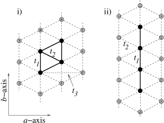
Figure 1: Triangular lattice structure and two possible clusters tiling the lattice. i) 4-site cluster including inter-chain self-energies. ii) 1D clusters neglecting inter-chain self-energies. Full circles and solid lines mark sites and bonds inside a clusters. Next-next-nearest neighbor hopping $t_{3}$ is only drawn once for clarity. In the case of the $t_{2g}$ manifold each lattice site consists of three orbitals.

After having constructed the low-energy Hamiltonian using ab initio techniques, we use the VCApo.ai.03 ; pott.03.epjb2 in order to calculate the spectral function of this model. Since we deal with an effective low-energy Hamiltonian that involves no other uncorrelated ligand states (O-$p$, Cl-$p$), but only the correlated Ti-$t_{2g}$ orbitals, the application of VCA is straightforward, and is from a technical point of view exactly equivalent to standard multi-orbital calculations for Hubbard-model Hamiltonians. The only difference is that the non-interacting part is determined by the procedure discussed in the previous subsection. Furthermore, since there are no explicit ligand states in the Hamiltonian, there is no need for a double-counting correction. It gives just a constant shift in energy which can be absorbed in the chemical potential.

As mentioned in the introduction, the VCA is a quantum cluster method capable of treating strong short-ranged correlations. The main idea is to approximate the self-energy of the original model, which is defined on an infinite lattice, by the self-energy of a finite cluster, the reference system. The variational principle states that the optimal solution is given by the stationary points of the grand potential $\Omega[\Sigma]$ as a function of the self-energy $\Sigma$. Parametrizing the self-energy by the single-particle parameters ${\mathbf{t}}^{\prime}$ of the reference system, we can write the grand potential as

$$\Omega({\mathbf{t}}^{\prime})=\Omega^{\prime}+\mbox{Tr}\ln({\mathbf{G}}_{0,{\mathbf{t}}}^{-1}-{\mathbf{\Sigma}}({\mathbf{t}}^{\prime}))^{-1}-\mbox{Tr}\ln{\mathbf{G}}_{{\mathbf{t}}^{\prime}}\>,$$ (4)

where $\Omega^{\prime}$ and ${\mathbf{G}}_{{\mathbf{t}}^{\prime}}$ are respectively the grand canonical potential and the Green’s function of the reference system and ${\mathbf{G}}_{0,{\mathbf{t}}}$ is the non-interacting Green’s function of the physical (lattice) system. The stationary condition reads

$$\frac{\partial\Omega}{\partial{\mathbf{t}}^{\prime}}\Big{|}_{{\mathbf{t}}^{\prime}={\mathbf{t}}^{\prime}_{\rm opt}}=0\;.$$ (5)

It is important to note that the interaction parameters are not variational parameters, since, by construction of the VCA, the interaction terms of the reference system and the original lattice model must not differ. In this study, we restrict ourselves to local interactions only since the VCA in its strict sense cannot be used for models with non-local interactions without further approximations.

In its spirit, the VCA is closely related to the dynamical mean-field theory (DMFT), where in the latter case the self-energy is obtained from an impurity problem.

The actual VCA calculation is done in the following steps. First, we determine the ground state of the reference system, i.e. a cluster of finite size as depicted in Fig. 1. The interacting Green’s function is calculated, and since the non-interacting Green’s function of the reference system is known, the self-energy can readily be obtained using Dyson’s equation. Using the grand potential $\Omega^{\prime}$ of the reference system, the Green’s function ${\mathbf{G}}_{{\mathbf{t}}^{\prime}}$, and the self-energy ${\mathbf{\Sigma}}({\mathbf{t}}^{\prime}))$, Eq. 4 is evaluated using the technique of $Q$-matrices.ai.ar.06.2 Note that the Green’s functions ${\mathbf{G}}_{0,{\mathbf{t}}}$, ${\mathbf{G}}_{{\mathbf{t}}^{\prime}}$ and the self-energy ${\mathbf{\Sigma}}({\mathbf{t}}^{\prime})$ in Eq. (4) are matrices not only in site and spin indices, but also carry an orbital index. In fact, this is the only difference of the application of VCA in the present case compared to the numerous previous applications to the single-band Hubbard model.

As a reference system solver, we use the Band-Lanczos exact diagonalization technique at zero temperature, which means that for the full $t_{2g}$ manifold, we can easily consider clusters with at most 4 sites, yielding a 12-orbital Green’s function ${\mathbf{G}}_{{\mathbf{t}}^{\prime}}$. For the single-band model, we consider clusters up to 12 sites. We exploit particle number and spin conservation, therefore the sizes of the largest Hilbert spaces that we have to consider are $N=14520$ states in the 4-site multi-orbital case, and $N=853776$ states in the 12-site single-orbital case, respectively. Since we are considering an exact diagonalization method for solving the cluster problem, all interactions in the Hamiltonians Eq. (2) and Eq. (3) are treated exactly and on the same footing. This is a clear advantage compared to, e.g., using the Hirsch-Fye quantum Monte-Carlo method as impurity solver, since in the latter case approximations to the interaction terms of the Hamiltonian have to be done.qmc

The VCA approach has been tested thoroughly and used successfully for many investigations in recent years. Several studies on the cuprate-based high-temperature superconductors have shown that this approach can reproduce salient features of these materials, such as the ground-state phase diagram,se.la.05 ; ai.ar.05 ; ai.ar.06 ; ai.ar.06.2 or the opening of the pseudogap at low hole doping, accompanied with the occurrence of Fermi arcs,se.tr.04 ; ai.ar.06 in very good agreement with experiments and results obtained by the cellular dynamical mean-field theory (CDMFT) (see, e.g, Refs. tr.ky.06, ). Recently, the VCA could also reproduce the pairing symmetry of the iron-based superconductors.da.mo.08

The VCA has also been used for multi-orbital systems, which is relevant for the combination with ab-initio methods. On the pure methodological level, the metal-insulator transition in infinite dimensions was studiedin.ko.05 ; in.ko.07 , and very good agreement with dynamical mean-field calculations was found. An application to real materials was done in Refs. ed.07, ; ed.08, , where the compounds NiO, CoO, and MnO have been studied and very good agreement with experimental photo-emission data has been found.

Details on the practical implementation of the VCA, including tests and benchmarking, can be found in Refs. po.ai.03, ; pott.03.epjb1, ; po.05.ass, ; ai.ar.06.2, ; ba.ha.08, ; se.08u, .

In general, all the single-particle parameters ${\mathbf{t}}^{\prime}$ are variational parameters of the VCA. In practice, one chooses a physically motivated subset in order to keep the numerical calculations feasible. Here we make the following choice. For a thermodynamically consistent description of the densities, it is crucial to consider the onsite energies, i.e. the local terms of the single-particle Hamiltonian $\varepsilon_{\alpha}^{\prime}\equiv(t_{ii}^{\alpha\alpha})^{\prime}$, as variational parameters.ai.ar.06 We define the average $\varepsilon^{\prime}=\frac{1}{2}(\varepsilon_{xy}^{\prime}+\varepsilon_{yz}^{\prime})$ and the crystal-field splitting $\Delta_{\rm cf}^{\prime}=\varepsilon_{yz}^{\prime}-\varepsilon_{xy}^{\prime}$, which are then used as the variational parameters of the VCA. Note that in the single-band case, Eq. (3), one has to deal with $\varepsilon^{\prime}$ only. One has to be aware that the variational parameter $\Delta_{\rm cf}^{\prime}$ does not impose an artificial orbital polarization of the system, since it is a parameter in the variational procedure and no physical external field. Hence, using $\varepsilon^{\prime}$ and $\Delta_{\rm cf}^{\prime}$, the orbital occupancies are determined in a fully self-consistent way.

The main property investigated in this work is the single-particle spectral function which we define as

$$A({\mathbf{k}},\omega)=-\frac{1}{\pi}{\rm\>tr\>Im\>}{{\mathbf{G}}}({\mathbf{k}},\omega)\;,$$ (6)

Since we broke the translational invariance of the system by introducing the cluster tiling, a proper periodization of the lattice quantities is needed in order to restore translational symmetry, an issue also important in cluster DMFT calculations.bi.pa.04 Here, we choose to use the periodization of the Green’s function since the periodization of the self-energy gives unphysical results in the insulating phase.se.08u In other words, starting from the Green’s function that depends on two momenta, ${{\mathbf{G}}}({\mathbf{k}},{\mathbf{k}}^{\prime},\omega)$, one restores the fully translationally invariant Green’s function ${{\mathbf{G}}}({\mathbf{k}},\omega)$, by neglecting the off-diagonal elements, and taking ${\mathbf{k}}={\mathbf{k}}^{\prime}$ only. It has been shown that this is a well justified approximation to calculating the momentum-dependent spectral function.se.pe.00 The Green’s function ${\mathbf{G}}$ is in general a matrix in orbital indices and $A({\mathbf{k}},\omega)$ is given by the trace over the orbital degrees of freedom.

III Results

III.1 Full $t_{2g}$ model vs. effective one-band model

Figure 2: Comparison of the single-particle spectral function of the $t_{2g}$ model (top) and the single-band model (bottom), both calculated with a $2\times 2$ reference system, see Fig. 1 i). Parameters are $U=3.3$ eV, $J=0.5$ eV. For the hopping parameters see text. The chemical potential has been chosen such that i) the system is insulating with $n=1.0$, and ii) the position of the occupied states coincide in both calculations. Lorentzian broadening of $\eta=0.02$ eV was used.

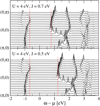
Figure 3: (Color online) Comparison of the spectral function of the $t_{2g}$ model for two different sets of interaction parameters. Top: $U=4.0$ eV, $J=0.7$ eV. Bottom: $U=4.0$ eV, $J=0.5$ eV. The vertical dashed lines mark the edges of the single-particle gap. Lorentzian broadening of $\eta=0.02$ eV was used.

Before we come to a detailed analysis of the single-band model, we first want to check the validity of the restriction to the lowest $d$-orbital.

For this reason, we performed ab initio calculations to determine the full single-particle Hamiltonian of the system. Since Ti³⁺ is in a $3d^{1}$ configuration, the $e_{g}$ orbitals are unoccupied and can be projected out, and the full kinetic Hamiltonian is downfolded to the threefold degenerate $t_{2g}$ manifold. Results show, that the system exhibits a strong anisotropy, with the largest hopping integrals in the crystallographic $b$-direction, see Fig. 1, almost one order of magnitude larger than the other transfer integrals. Moreover, the threefold degeneracy is lifted and the manifold split into the lower $d_{xy}$ and the higher $d_{xz}$ and $d_{yz}$ orbitals. Note that for the orbital designation we consider the same local reference frame as in Ref. da.li.05, ; ho.si.05, . The crystal-field splitting between the ground state and the first excited state obtained from LDA is about 0.42 eV. This theoretical value is in reasonable agreement with experimental results.ru.ba.05 ; za.de.06 Despite this splitting, the orbital sector is not fully polarized in the LDA calculations, and the occupation of $d_{xy}$ is about 0.49, with 0.51 electrons in the other two orbitals.

In order to perform our LDA+VCA calculations, we take the downfolded Hamiltonian of the ab initio calculations, and add the interaction and exchange terms according to Eq. (2). In the upper panel of Fig. 2 we show the results for the spectral function, Eq. (6), calculated for this three-band $t_{2g}$ model using typical parameters $U=3.3$ eV and $J=0.5$ eV. The bands which are located just above the Fermi level, between roughly 0.5 eV and 2.0 eV, have $d_{xz}$ and $d_{yz}$ character, and remain almost unchanged by the strong interactions.

The behavior of the $d_{xy}$ orbital is strikingly different. It splits into two bands that can be identified with the lower and upper Hubbard band, located roughly around $-1.0$ eV and 2.5 eV, respectively. By inspecting the terms of the Hamiltonian related to the crystal-field splitting, i.e. $H_{\rm cf}=\Delta_{\rm cf}\sum_{i}(n_{yz}+n_{zx}-n_{xy})$, we can calculate the orbital polarization $p=\partial\Omega/\partial\Delta_{\rm cf}$. We find a value of $p=-0.99$, meaning that the system is almost perfectly polarized into the $d_{xy}$ orbital, which is in agreement with recent LDA+CDMFT calculations.da.li.07 Interestingly, this polarization is found without any sizable increase of the crystal-field splitting in the variational procedure, i.e., $\Delta_{\rm cf}\approx\Delta_{\rm cf}^{\prime}$, but it is only due to the inclusion of strong local interactions.

This result gives rise to the question, to which extent a single-band Hubbard model can describe the occupied states relevant for comparison with ARPES. We took parameters from a full downfolding to the Ti $d_{xy}$ orbital only, cf. first column of Table I in Ref. da.va.04, . Using the same value of $U=3.3$ eV we calculate the spectral function for Hamiltonian Eq. (3). The results are shown in the lower panel of Fig. 2. In order to avoid effects coming from different cluster sizes, we used also a $2\times 2$ cluster for this comparison. Note that below the Fermi level the agreement between the single-band model and the $d_{xy}$ part of the $t_{2g}$ model is excellent. For this reason we conclude that for a comparison of spectra with experimental ARPES measurements the Hamiltonian Eq. (3) is a reasonable starting point.

Before turning to a more detailed analysis of the spectra obtained from Eq. (3), let us briefly discuss the single-particle gap $\Delta$, defined as the energy difference between the lowest unoccupied and the highest occupied state. For a comparison of this quantity with experiments, it is clear that the single-band model is not sufficient, since it does not describe the excited states in the $t_{2g}$ manifold. However, we extracted the gap $\Delta$ from the spectral function of the $t_{2g}$ model, for different values of $U$ and $J$. We find that the main quantity that determines the gap is the inter-orbital Coulomb interaction $U^{\prime}=U-2J$, and we get $\Delta\approx 1.2$ eV for $U=3.3$ eV, $J=0.5$ eV. In Fig. 3 we plot the spectral function for different sets of interaction parameters, and find $\Delta\approx 1.4$ eV for $U=4$ eV, $J=0.7$ eV, and $\Delta\approx 1.9$ eV for $U=4$ eV, $J=0.5$ eV. All these values for the gap are a bit smaller than the experimental charge gap of about 2 eV,ru.ba.05 but nevertheless in reasonable agreement.

III.2 Spectral weights in the single-band Hubbard model

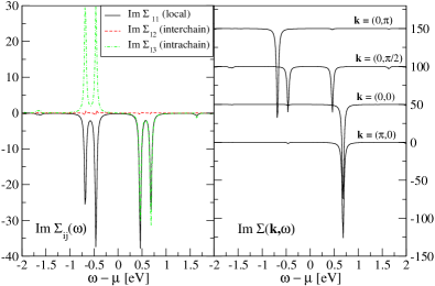
Figure 4: (Color online) Imaginary part of the self-energies on a reference system consisting of two coupled 4-site chains. Left panel: Real space $\Sigma_{ij}(\omega)$. Solid line: Local/onsite self-energy $\Sigma_{11}(\omega)$. Dashed line: Inter-chain self-energy $\Sigma_{12}(\omega)$. Dash-dotted line: Intra-chain self-energy $\Sigma_{13}(\omega)$. Right panel: Self-energy for selected momenta of the cluster. Momenta are indicated in the plot, and a vertical shift between momenta has been introduced for improved presentation. The self-energy shows causality (negative definite), almost no dependence in $a$-direction, and strong dependence in $b$-direction. Lorentzian broadening of $\eta=0.02$ eV was used in both plots.

We have shown in Sec. III.1 that the occupied states of the $t_{2g}$ manifold are well reproduced by a single-band Hubbard model. In this section we want to investigate the spectral function of Eq. (3) in more detail. As mentioned above, we focus on the effect of the additional two-dimensional hopping processes on the quasi-one-dimensional behavior of TiOCl.

First, we want to determine the strength of the correlations along the qualitatively different bonds of the lattice, Fig. 1. This can be done best by inspecting the self-energy $\Sigma_{ij}(\omega)$, which is, in VCA, a quantity defined on the reference system and, thus, can be readily obtained. The results for three selected matrix elements are shown in Fig. 4, calculated on an $2\times 4$ cluster. This cluster consists of two coupled 4-site chains in $b$-direction. In other words, a cluster similar to the one depicted in Fig. 1 i) but with doubled extension in $b$-direction. It is obvious that local ($\Sigma_{11}(\omega)$) and intra-chain correlations ($\Sigma_{13}(\omega)$) are strong, but the correlations between adjacent chains ($\Sigma_{12}(\omega)$) are orders of magnitude weaker. In addition, we show in the right panel of Fig. 4 the Fourier transformation of the self-energy, for momenta accessible at this small cluster. Again, the influence of momenta perpendicular to the chains is hardly visible in the self-energy, whereas it shows significant momentum dependence in the chain direction. This leads to the conclusion that the spectra of TiOCl should be governed by 1D correlations, modified by single-particle effects due to the coupling of the chains.

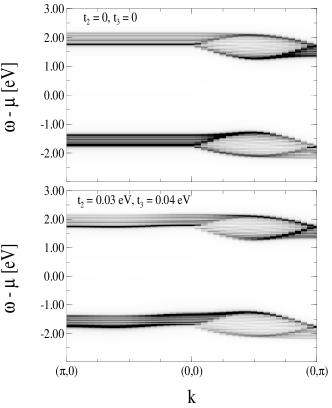
Figure 5: Spectral function of the single-band model with a 12-site chain as reference system. Top: No coupling between chains. Bottom: Inclusion of interchain coupling parameters obtained from LDA-downfolding. Dark areas mark large spectral weight. Lorentzian broadening of $\eta=0.02$ eV was used. The horizontal striped structures occur due to the breaking of translational invariance in the cluster approximation.

Motivated by this result, we use from now on a $1\times 12$ cluster as reference system. Since the VCA approximates the interacting Green’s function as ${\mathbf{G}}(\omega)^{-1}={\mathbf{G}}_{0,{\mathbf{t}}}^{-1}-{\mathbf{\Sigma}}(\omega)$ with ${\mathbf{G}}_{0,{\mathbf{t}}}$ the non-interacting Green’s function of the model Hamiltonian and ${\mathbf{\Sigma}}(\omega)$ the cluster self-energy, it is easy to see that the inter-cluster coupling is treated in a single-particle (i. e., non-interacting) manner, since it enters just via ${\mathbf{G}}_{0,{\mathbf{t}}}$. On the other hand, this procedure gives the best possible description of the correlation effects along the chains in $b$-direction.

In Fig. 5 we show a density plot of the spectral function of the Hamiltonian Eq. (3) for $U=3.3$ eV. In the upper part we included only the intra-chain hopping $t_{1}=-0.21$ eV in the calculation, leading to flat bands in $a$-direction, i. e., from $(\pi,0)$ to $(0,0)$, since in this case the chains are decoupled. By including additional inter-chain parameters $t_{2}=0.03$ eV and $t_{3}=0.04$ eV as given in Ref. da.va.04, , we notice a slight dispersion in $a$-direction. In $b$-direction, however, the band positions remain almost unchanged; we find only changes in the spectral weights. Since this cannot be seen clearly in the density plots, we show in Fig. 6 the evolution of the spectral function at the $\Gamma$ point $\mathbf{k}=(0,0)$ when longer-ranged hopping processes are included.

Figure 6: Spectral function $A(k=0,\omega)$ at the $\Gamma$ point. Top left: without inter-chain coupling. Top right: Including nearest-neighbor inter-chain coupling $t_{2}$. Bottom right: Including next-nearest-neighbor inter-chain coupling $t_{3}$. For comparison, bottom left: next-nearest-neighbor hopping along the chain, but no inter-chain hopping. Lorentzian broadening of $\eta=0.02$ eV was used.

The upper left panel (a) is the spectral function for decoupled chains with the spin-charge separation clearly visible. At the $\Gamma$ point the holon band is located around $-1.72$ eV, and the spinon band around $-1.39$ eV. Including the nearest neighbor inter-chain hopping $t_{2}$ leads to a significant redistribution of spectral weight from the holon to the spinon band, i. e., from higher to lower binding energies, see the upper right panel (b). This effect is even enhanced when the next-nearest inter-chain hopping $t_{3}$ is included, as shown in the lower right panel (d). Here the spectral weight of the low binding energy (’spinon’) excitation is comparable to the weight of the high binding energy (’holon’) excitation for decoupled chains in panel (a), and vice verse. At this point we would like to mention, that in a strict sense the terminology ’spinon’ and ’holon’ is not applicable any more, since these are properties of purely one-dimensional systems. Anyway, since the spectra resemble to some extent 1D systems, we still use these terms to distinguish the different excitations.

From Fig. 6 it is clear that the inclusion of inter-chain processes enhances the asymmetry of the $\mathbf{k}$-resolved spectra. The low-lying excitation near the $\Gamma$ point is strongly enhanced, whereas there is no spectral weight transfer to lower binding energies visible around $(0,\pi)$. Note that we define the spectrum to be symmetric if the main excitations at $\mathbf{k}$-vector $(0,0)$ and $(0,\pi)$ are located at the same binding energy.

One may ask if it is possible to get a similar spectral weight distribution by using only the purely one-dimensional Hubbard model, but including longer-ranged intra-chain hopping processes as given by the ab initio calculations. In fact, the next-nearest-neighbor hopping term along the chain, $t_{4}$, is of similar size of the inter-chain hoppings.da.va.04 The result for the spectral function at the $\Gamma$ point in this pure 1D case is shown in the lower left panel (c) of Fig. 6. From this result it is obvious that one can not get an excitation at binding energies of roughly $-1.4$ eV, as seen in experiments. On the contrary, the spectral weight of the excitation at the higher binding energy of about $-1.8$ eV is even enhanced in the one-dimensional treatment when longer-ranged hopping processes are included.

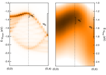
Figure 7: (Color online) Comparison of the theoretical spectral function (left) with the experimental ARPES spectra (right). Only the $b$-direction is shown. Lorentzian broadening of $\eta=0.02$ eV was used. The vertical dashed line marks momentum $(0,\pi/2)$, and the band widths $w_{b}$ and $w_{b}^{\prime}$ are indicated. Dark areas mark large spectral weight, the color scale is normalized in each plot separately.

Our results support the description of TiOCl as a layered two-dimensional compound with strong anisotropy, also on the level of correlations. There is finite dispersion also perpendicular to the chains, but a backfolding of the bands can only be seen along the chains, where correlations are dominant.

Let us now comment on the relation of our results to ARPES data. Experiments showho.si.05 that the dispersion in TiOCl shows a strong asymmetric behavior along the crystallographic $b$ direction, see also the right plot of Fig. 7. The binding energy of the lowest-lying band around $\mathbf{k}=(0,0)$ is about $-1.5$ eV, whereas around $\mathbf{k}=(0,\pi)$ it is about $-2.0$ eV. First attempts to describe the dispersions within ab initio calculations were not successful. Standard LDA calculations do not produce the backfolding of the bands induced by short-range spin fluctuations, and spin-polarized LSDA+U calculations cannot account for the asymmetry of the spectra. Also the spectra of the one-dimensional Hubbard model calculated within the dynamical density-matrix renormalization group (DDMRG) do not reproduce the experimental spectral weight distribution.ho.si.05 However, as can be seen in Fig. 7, our new results show that the Hubbard model can indeed give a good description of the asymmetry, since the inter-chain processes give rise to a spectral weight transfer from the holon to the spinon band around the $\Gamma$ point, and therefore make the band structure more asymmetric.

In order to compare our results more quantitatively, we extract the following numbers related to the band widths of the spectra. The first one, $w_{b}$, is the difference of the binding energies at $(0,\pi/2)$ and $(0,\pi)$ and is a measure for the overall band width. The second one, $w_{b}^{\prime}$, is defined to be the difference in binding energies between $(0,\pi/2)$ and $(0,0)$. The larger the difference between these two quantities, the larger is the asymmetry of the spectra. From experimentsho.si.07 we extract $w_{b}\approx 0.47$ eV and $w_{b}^{\prime}\approx 0.17$ eV, and for the calculated spectra we get $w_{b}\approx 0.50$ eV and $w_{b}^{\prime}\approx 0.09$ eV. Comparing theory and experiment, we see that the overall band width $w_{b}$ is well reproduced by the calculation, but the asymmetry is even a bit more pronounced in the theoretical spectra, resulting in a smaller value of $w_{b}^{\prime}$. This result may be improved by including more longer-ranged hopping processes. Although they decrease rapidly with distance, they can change the band widths within a few percent.

By inspecting Fig. 7 it is obvious that the width of the spectra is much larger in the ARPES data than in the calculated spectra. The most important reason for that is that our calculations are done at $T=0$, using exact diagonalization techniques. Therefore there are no life-time effects due to finite temperatures included in our calculations. Moreover, additional coupling to lattice degrees of freedom could also lead to a smaller life time, and hence broader excitations.

In summary, our results imply that it is important to include the inter-chain couplings at least on a single-particle non-interacting level into the effective model, in order to improve the description of the experimental spectra, although the strong correlations are constricted mainly to the chains.

With our work we could fill the gap left by previous theoretical studies regarding the momentum-resolved single-particle spectral function of TiOCl. There are, though, still some open questions. For example, we do see clear signatures of spin-charge separation in our calculated spectra, which have not been found experimentally. Also the so-called shadow band, dispersing at around $-2$ eV has not been seen in the ARPES spectra. A reason for this can be a very small relative spectral weight of the high-energy band that cannot be resolved in experiment. In our calculation we also did not include the lattice degrees of freedom, which are supposed to be very important in TiOClpi.va.07 , driving the spin-Peierls phase transition. These phonons can also lead to a smearing of the peak structure of $A(\mathbf{k},\omega)$.

Finally, we want to comment also on the differences between the ARPES spectra of TiOCl and TiOBr. Experiments, supplemented with band structure calculations, have shownle.ch.05 ; ho.si.07 that in the latter compound the intra-chain couplings are weaker and the inter-chain couplings stronger compared to TiOCl,le.ch.05 e. g., $t_{1}$ decreases from $-0.21$ eV to $-0.17$ eV, whereas $t_{3}$ increases from $0.04$ eV to $0.06$ eV. By inspecting the self-energies in a similar manner as we did in Fig. 4, we found that also for these parameter values the correlations are predominantly one-dimensional. There are only changes in the overall bandwidths, but no qualitative changes. For instance, the band width in $a$-direction is enhanced, but there are no signatures of strong inter-chain correlations resulting in a backfolding of the bands.

At this point we want to remark that, in particular for TiOBr, one should be very careful with the use of the spinon/holon terminology. Although there are no qualitative changes due to the enhanced couplings, they do change the band widths. Hence, quantitative analysis have to be done including these inter-chain couplings.

IV Conclusions

By combining ab initio calculations (LDA) and the variational cluster approximation, we could study for the first time the momentum-resolved spectral function including a realistic band structure and strong-correlation effects. In agreement with previous theoretical studies and experimental results, our calculations showed an almost complete polarization in the orbital sector, with 99% of the electrons occupying the Ti $d_{xy}$ orbital.

Since the orbital degree of freedom is quenched, we could use an effective single-band model for the investigation of the spectral properties. The most striking result of our study is that the inclusion of inter-chain hopping processes leads to a significant spectral weight redistribution around the $\Gamma$ point from higher to lower binding energies. This effect, which makes the spectrum more asymmetric with respect to the points $(0,0)$ and $(0,\pi)$, cannot be reproduced using only the hopping processes along the chains. This result suggests that the frustrated inter-chain couplingzh.je.08 is one of the main reasons for the strong asymmetry that has been found in experimental ARPES measurements. Moreover the calculated spectral features may be extended to a more general class of correlated coupled-chains systems.

An open question in TiOCl is still the role of phonons. Because of the vicinity of the system to a spin-Peierls instability, the phonons are supposed to be important in the system. Including these degrees of freedom, although theoretically very demanding, could further improve the results with respect to lineshapes and lifetimes of the excitations.

- (1) R. J. Beynon and J. A. Wilson, J. Phys.: Condens. Matter 5, 1983 (1993).
- (2) A. Seidel, C. A. Marianetti, F. C. Chou, G. Ceder, and P. A. Lee, Phys. Rev. B 67, 020405(R) (2003).
- (3) R. Rückamp, J. Baier, M. Kriener, M. W. Haverkort, T. Lorenz, G. S. Uhrig, L. Jongen, A. Möller, G. Meyer, and M. Grüninger, Phys. Rev. Lett. 95, 097203 (2005).
- (4) M. Shaz, S. van Smaalen, L. Palatinus, M. Hoinkis, M. Klemm, S. Horn, and R. Claessen, Phys. Rev. B 71, 100405(R) (2005).
- (5) J. Hemberger, M. Hoinkis, M. Klemm, M. Sing, R. Claessen, S. Horn, and A. Loidl, Phys. Rev. B 72, 012420 (2005).
- (6) A. Schönleber, S. van Smaalen, and L. Palatinus, Phys. Rev. B 73, 214410 (2006).
- (7) E. T. Abel, K. Matan, F. C. Chou, E. D. Isaacs, D. E. Moncton, H. Sinn, A. Alatas, and Y. S. Lee, Phys. Rev. B 76, 214304 (2007).
- (8) V. Kataev, J. Baier, A. Möller, L. Jongen, G. Meyer, and A. Freimuth, Phys. Rev. B 68, 140405(R) (2003).
- (9) Y.-Z. Zhang, H. O. Jeschke, and R. Valentí, Phys. Rev. B 78, 205104 (2008).
- (10) C. A. Kuntscher, S. Frank, A. Pashkin, M. Hoinkis, M. Klemm, M. Sing, S. Horn, and R. Claessen, Phys. Rev. B 74, 184402 (2006).
- (11) C. A. Kuntscher, A. Pashkin, H. Hoffmann, S. Frank, M. Klemm, S. Horn, A. Schönleber, S. van Smaalen, M. Hanfland, S. Glawion, M. Sing, and R. Claessen, Phys. Rev. B 78, 035106 (2008).
- (12) Y.-Z. Zhang, H. O. Jeschke, and R. Valentí, Phys. Rev. Lett. 101, 136406 (2008).
- (13) S. Blanco-Canosa, F. Rivadulla, A. Pineiro, V. Pardo, D. Baldomir, D. I. Khomskii, M. M. Abd-Elmeguid, M. A. López-Quintela, and J. Rivas, Phys. Rev. Lett. 102, 056406 (2009).
- (14) M. Hoinkis, M. Sing, J. Schafer, M. Klemm, S. Horn, H. Benthien, E. Jeckelmann, T. Saha-Dasgupta, L. Pisani, R. Valentí, and R. Claessen, Phys. Rev. B 72, 125127 (2005).
- (15) M. Hoinkis, M. Sing, S. Glawion, L. Pisani, R. Valentí, S. van Smaalen, M. Klemm, S. Horn, and R. Claessen, Phys. Rev. B 75, 245124 (2007).
- (16) T. Saha-Dasgupta, R. Valentí, H. Rosner, and C. Gros, Europhys. Lett. 67, 63 (2004).
- (17) L. Pisani, R. Valentí, B. Montanari, and N. M. Harrison, Phys. Rev. B 76, 235126 (2007).
- (18) T. Saha-Dasgupta, A. Lichtenstein, and R. Valentí, Phys. Rev. B 71, 153108 (2005).
- (19) L. Craco, M. S. Laad, and E. Müller-Hartmann, J. Phys. Cond. Mat. 18, 10943 (2006).
- (20) T. Saha-Dasgupta, A. Lichtenstein, M. Hoinkis, S. Glawion, M. Sing, R. Claessen, and R. Valentí, New J. Phys. 7, 380 (2007).
- (21) M. Potthoff, M. Aichhorn, and C. Dahnken, Phys. Rev. Lett. 91, 206402 (2003).
- (22) M. Potthoff, Eur. Phys. J B 32, 429 (2003).
- (23) L. Chioncel, H. Allmaier, E. Arrigoni, A. Yamasaki, M. Daghofer, M. I. Katsnelson, and A. I. Lichtenstein, Phys. Rev. B 75, 140406 (2007).
- (24) O. K. Andersen and T. Saha-Dasgupta, Phys. Rev. B 62, R16219 (2000).
- (25) H. Allmaier, L. Chioncel, and E. Arrigoni, Phys. Rev. B 79, 235126 (2009).
- (26) In most calculations based on stochastic evaluations, the Hund term consists only of Ising-type interactions.
- (27) M. Aichhorn, E. Arrigoni, M. Potthoff, and W. Hanke, Phys. Rev. B 74, 235117 (2006).
- (28) D. Sénéchal, P. L. Lavertu, M. A. Marois, and A. M. S. Tremblay, Phys. Rev. Lett. 94, 156404 (2005).
- (29) M. Aichhorn and E. Arrigoni, Europhys. Lett. 72, 117 (2005).
- (30) M. Aichhorn, E. Arrigoni, M. Potthoff, and W. Hanke, Phys. Rev. B 74, 024508 (2006).
- (31) D. Sénéchal and A. M. S. Tremblay, Phys. Rev. Lett. 92, 126401 (2004).
- (32) A. Tremblay, B. Kyung, and D. Sénéchal, Low Temperature Physics 32, 424 (2006).
- (33) M. Daghofer, A. Moreo, J. A. Riera, E. Arrigoni, D. J. Scalapino, and E. Dagotto, Phys. Rev. Lett. 101, 237004 (2008).
- (34) K. Inaba, A. Koga, S.-I. Suga, and N. Kawakami, Phys. Rev. B 72, 085112 (2005).
- (35) K. Inaba and A. Koga, J. Phys. Soc. Jpn. 76, 094712 (2007).
- (36) R. Eder, Phys. Rev. B 76, 241103 (2007).
- (37) R. Eder, Phys. Rev. B 78, 115111 (2008).
- (38) M. Potthoff, Eur. Phys. J B 36, 335 (2003).
- (39) M. Potthoff, Adv. Solid State Phys. 45, 135 (2005).
- (40) M. Balzer, W. Hanke, and M. Potthoff, Phys. Rev. B 77, 045133 (2008).
- (41) D. Sénéchal, arXiv:0806.2690 (unpublished).
- (42) G. Biroli, O. Parcollet, and G. Kotliar, Phys. Rev. B 69, 205108 (2004).
- (43) D. Sénéchal, D. Perez, and M. Pioro-Ladriere, Phys. Rev. Lett. 84, 522 (2000).
- (44) D. V. Zakharov, J. Deisenhofer, H.-A. Krug von Nidda, P. Lunkenheimer, J. Hemberger, M. Hoinkis, M. Klemm, M. Sing, R. Claessen, M. V. Eremin, S. Horn, and A. Loidl, Phys. Rev. B 73, 094452 (2006).
- (45) P. Lemmens, K. Y. Choi, R. Valentí, T. Saha-Dasgupta, E. Abel, Y. S. Lee, and F. C. Chou, New J. Phys. 7, 74 (2005).