Competition and fragmentation: a simple model generating lognormal-like distributions

Abstract

The current distribution of language size in terms of speaker population is generally described using a lognormal distribution. Analyzing the original real data we show how the double-Pareto lognormal distribution can give an alternative fit that indicates the existence of a power law tail. A simple Monte Carlo model is constructed based on the processes of competition and fragmentation. The results reproduce the power law tails of the real distribution well and give better results for a poorly connected topology of interactions.

The astonishing similarity between biological and language evolution has attracted the interest of researchers familiar with analyze genetic properties in biological populations with the aim of describing problems of linguistics [1, 2, 3]. Their techniques, for instance, have succeeded in explaining some interesting features related to the coexistence of the about $7,000$ languages present on Earth.

More recently, the effort to connect evolutionary biology with linguistics has emerged into a study that describes the effects of competition between languages on language evolution. The work of Abrams and Strogatz in 2003 [4], who analyzed the stability of a system composed of two competing languages, can be considered as the starting point of this new research line. In the following years, other groups, simultaneously, developed new analytical and computational models [5, 6, 7, 8, 9, 10, 11, 12]. An overview of the fast increasing literature on language competition can be found in refs. [13, 14].

Languages are by no way static. They continuously evolve, changing, for example, their lexicon, phonetic, and grammatical structure. This evolution is similar to the evolution of species driven by mutations and natural selection [15]. Following the common picture of biology [16], changes in the language structure may be seen as the result of microscopic stochastic changes caused by mutations. Natural selection, which may be caused by competition between individuals, positively selects some of these small changes, depending on their reproductive success. A sequence of macroscopic observations corresponds to such a microscopic picture. In language evolution, these macroscopic events are, for instance, the origination of two languages from an ancestor one - for example, the emergence of the Romance languages from Latin - or the extinction of a language.

In this work we model the evolution of languages from a macroscopic point of view. More precisely, the microscopic processes responsible for the differentiation of one language into two new languages are not implemented here. Effectively, we neglect the microdynamics that generates language changes, at the level of individuals, and we just describe their effect on extinction and differentiation at the level of languages, throughout a phenomenological mechanism of growth and fragmentation. Language change is determined by the dynamics of the size of its population. The fact that rare languages are less attractive for people to both learn and use is the mechanism considered as the origin of these population size changes. Consequently, this mechanism introduces a sort of frequency dependent reproductive success for different languages. Statistical data supporting this conjecture can be found in Ref. [17]. Languages documented as declining are negatively correlated with population size. This phenomenon is similar to the Allee effect in biology [18]. With a simple computational model, based on the above described mechanisms, we compare simulation results with empirical data of the distribution of population sizes of languages (DPL) of Earth’s actually spoken languages [19] (see Fig. 1).

Several attempts have recently been made to reproduce the DPL. Two works focused on the apparently lognormal shape of the DPL. Tuncay [20] described language differentiation by means of a process of successive fragmentations, in combination with a multiplicative growth process. In a recent paper by Zanette [21], the dynamics of language evolution is considered as a direct consequence of the demographic increase of the speaker populations, which is modeled by means of a simple multiplicative process. Unsurprisingly, these models obtain pure lognormal distributions for the DPL, as expected from the application of the central limit theorem for multiplied random variables [22, 23]. Unfortunately, the DPL is known to significantly differ from a pure lognormal shape [17].

The Schulze model [8] relies on ideas already successfully applied to model biological evolution. Languages are identified by a bit string that represents their characteristic features. New languages are produced by mutations of these features and small languages are discriminated by competition. These simulations, during the transient towards the stationary state, are able to generate data with a distribution similar to the DPL. A review of the Schulze model and its application to different problems connected to language interaction can be found in Ref. [14].

Another model, the Viviane model, simulates human settlement on an unoccupied region. Languages suffer local mutations, until the available space becomes completely populated [12]. The introduction of a bit string representation into the Viviane model was able to generate new results which reproduce the DPL over almost the entire range well, except for large language sizes [24, 25]. The bit string approach gives an explanation for the deviation of the DPL from a lognormal distribution for small population sizes. The DPL changes its shape depending on the method used to distinguish different languages from dialects. When restricting the comparison between languages to be based on a small number of different features in language structure, the deviation for small language populations appears. This interpretation was confirmed by using a simple model [26] that neglects the geographic effects present in the Viviane model.

A thorough look at the DPL may suggest that the deviations from the lognormal shape could be due to power law decays [27]. We investigate this idea by fitting the DPL with a double-Pareto lognormal distribution and additionally comparing it to the simulation results of our new model.

The paper is organized as follows. First we analyze the DPL and show that the double-Pareto lognormal distribution [28, 29] gives an alternative fit. The next section introduces the computational model. In the last two sections, the simulation results are presented and the conclusions are given, respectively.

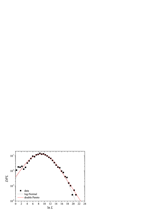
Figure 1: DPL distribution and respective fits with a double-Pareto lognormal distribution (continuum line) and lognormal one (dotted line). We counted the number of languages with speaker populations between $\exp(0.625n)$ and $\exp(0.625(n+1))$ for $n=0,1,2,3,...$. Although the double-Pareto lognormal distribution shows the same deviation from the real data for small values of $L$, it presents a better adjustment of the whole curve when in comparison to the log-normal fit (see $D_{KS}$ values in the text). In particular, it is possible to see how the fat tail for languages with a big population size is well fitted by a power law.

1 Statistical analysis of the distribution of languages

Reference [19] provides the number of people speaking a given language as their own mother tongue. There, 6,912 different languages have been classified and for 6,142 of them their speaker population was estimated. In the data set of 6,142 languages we also verify a big difference between the median, $6000$ speakers, and the average of the number speakers of a language, circa $1.052\times 10^{6}$ speakers. This discrepancy is related to the fact that only 326 languages have at least one million speakers. When they are assembled, these languages account for more than $95\%$ of world’s population with the remaining 5816 ($94.6\%$) languages encompassing the left-over speaking population. This draws attention to the fat tailed behaviour of the distribution of the number of speakers. Starting from these data, we make a histogram by counting the number of languages with population size enclosed in a bin with values between $\exp(0.625n)$ and $\exp(0.626(n+1))$ where $n=0,1,2,...$. This distribution defines the DPL. A pure lognormal shape can be described by,

$$DPL_{\textrm{lognormal}}(L)=A\exp\left[-\frac{(\ln L-\mu)^{2}}{2\,\sigma^{2}}\right]$$ (1)

where $A$, $\mu$ and $\sigma$ are the parameters of the distribution. A lognormal distribution corresponds to a parabola in a double–logarithmic plot (see Fig. 1).

In order to calculate the parameter values by maximum log-likelihood estimation we have to transform the distribution to obtain a probability density function. As the size of the bins in the DPL increases exponentially, the frequency of languages with a certain population size is calculated by dividing the DPL by the bin width which leads to,

$$c(L)=\frac{1}{\sqrt{2\,\pi\,\sigma^{2}}\,L}\exp\left[-\frac{(\ln L-\mu)^{2}}{2\,\sigma^{2}}\right]~{},$$ (2)

after further normalization in order to satisfy $\sum_{L}c(L)=1$.

The fit by maximum log-likelihood estimation with the lognormal distribution of eq. (2) gave the parameter values $\mu=8.70$ and $\sigma=3.20$ with a Kolmogorov-Smirnov distance of $D_{KS}=0.0253$. These values of the lognormal distribution are the same as the ones obtained in ref. [17], where $\log_{10}(L)$ was used instead of $\ln(L)$.

Unfortunately, as stated before, the DPL of real data is known to significantly differ from lognormality [17] and deviations can be easily observed for small and large values of $L$.

In particular, a thorough look on the DPL shows that it does not seem to decay exponentially. Hence, we have tried to fit the data using a distribution that can account for such a power law decay. As both tails could show power laws, we assumed the so-called double Pareto lognormal distribution, introduced by Reeds [28, 29],

$$c\left(L\right)=\frac{\alpha\,\beta}{\alpha+\beta}\left(A\,L^{-\alpha-1}\Phi\left[\frac{\ln L-\nu-\alpha\,\tau^{2}}{\tau}\right]+B\,L^{\beta-1}\Phi^{\prime}\left[\frac{\ln L-\nu+\beta\,\tau^{2}}{\tau}\right]\right),$$ (3)

where $\Phi\left(x\right)$ represents the cumulative distribution function of the normal distribution up to $x$ ($\Phi^{\prime}\equiv 1-\Phi\left(x\right)$), $A=\exp\left[\alpha\nu+\alpha^{2}\frac{\tau^{2}}{2}\right]$, and $B=\exp\left[-\beta\nu+\beta^{2}\frac{\tau^{2}}{2}\right]$.

In this case, using the maximum log-likelihood procedure, we have estimated the following values for the function parameters: $\alpha=0.682$, $\beta=0.603$, $\tau=2.33$, and $\nu=8.89$. This set of parameters yields $D_{KS}=0.0198$ which is slightly smaller than the distance presented by the log-normal fit. With these values we can compute the critical $P$ value, $P_{c}$, which is given by

$$\sqrt{\frac{-\ln\left(\frac{P_{c}}{2}\right)}{2\,N}}=D_{KS}.$$ (4)

The closer $P_{c}$ is to zero, the poorer the fit is. With the values presented previously we have $P_{C}\simeq 1.6\times 10^{-2}$ for the fit for Eq. (3) and $P_{C}\simeq 8\times 10^{-4}$ for the log-normal adjustment. This fact suggests that the double Pareto distribution allows a better description of real data. Figure 1 shows the results of this analysis comparing the corresponding DPLs.

It is likely to obtain better results by using a fitting function with a larger number of adjustable parameters. The Akaike information criterion [30] provides an estimation whether the introduction of new parameters into the fitting procedure is useful,

$$AIC=2k+N\log{\frac{RSS}{N}}~{}.$$ (5)

$k$ denotes the number of fitting parameters and $RSS$ is the residual sum of squares. Smaller values of this criterion correspond to better results. We obtain $AIC=-10.25$ for the fitting with the lognormal function and $AIC=-12.08$ for the one with the double-Pareto lognormal function.

2 Interaction versus fragmentation

This section introduces our model. As we stated before, we describe the behavior of languages on the macroscopic scale of sub-populations, neglecting the languages internal structure, constituted by the speaking preferences of each individual. Each language $i$ is characterized exclusively by the number of its speakers $L_{i}$. The origination of one new language is obtained throughout fragmentation. Fragmentation is implemented as follows: at each time step, each language can break into two new languages with a fixed probability $F$:

$$L_{i}(t)\longrightarrow L_{i}(t+1)=\frac{1}{2}L_{i}(t)\,,\,L_{new}(t+1)=\frac{1}{2}L_{i}(t)\,.$$ (6)

For the sake of simplicity, the two new languages contain exactly half of the population of the ancestor language (fragmentations into two parts of unequal size do not alter the qualitative shape of the distribution of the fragments size). Taking into account only the fragmentation process, the number of languages, $N_{L}$, increases until each language has only one speaker. For large numbers of $N_{L}$, there is an interval, during the time evolution, when the population distribution displays a pure lognormal shape.

It is interesting to remember that a simple soluble model analog to this fragmentation process is the discrete sequential fragmentation of a segment. In this case, through a rate equation approach, it is possible to show that an explicit asymptotic solution is given by a lognormal distribution. This is independent on the number of pieces of each breaking event [31].

The interaction between languages is implemented by a term that controls the growth of each language in dependence of its relative population size. At each time step, the population of each language $i$ follows the rule:

$$L_{i}(t+1)=\cases{L_{i}(t)+\frac{I}{N_{Tot}(t)}\sum\limits_{j\textrm{\tiny: NN or all}}(L_{i}(t)-L_{j}(t))-\frac{N_{Tot}(t)}{V}&for $L_{i}(t+1)\geq 1$\cr\textrm{language removed}&otherwise\cr}$$ (7)

where $L_{i}(t)$ denotes the number of speakers of language $i$ at time step $t$, $I$ the interaction strength and $N_{Tot}(t)=\sum\limits_{i=0}^{N_{L}(t)}L_{i}(t)$ is the total number of speakers. The second term, which can be positive or negative, enhances the reproductive success of the languages with more speakers, and causes the decrease of the number of rare language speakers. The third term, which is controlled by the parameter $V$, is a cause of random death that avoids the unlimited growth of the population. The term limits the growth of each language to have less than $V$ speakers. It is important to notice that this third term is necessary because the second one causes an uncontrolled growth in the total population. In fact, the second term does not conserve the total population because languages with less than one speaker ($L_{i}(t)<1$) are removed from the simulation.

We perform the simulations over two different topologies. In the first, the languages are ordered in a chain, with periodic boundary conditions, and interact with their nearest neighbors (NN). New languages, generated by fragmentation, are placed between the ancestor language and the following one. This implementation describes restricted local interactions, that can only happen between neighbor languages, in a 1-dimensional space.

In the second implementation, the interaction is carried out between all languages, in a mean field like model. For each iteration, every single language interacts with the whole set of languages. This model corresponds to the ideal case of a fully connected world, without geographic constraints.

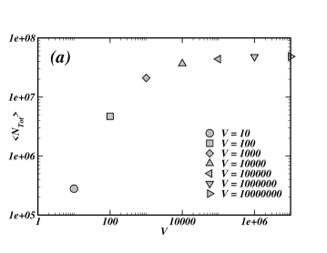
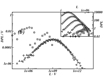
Figure 2: Local interactions. (a): Averaged total population $<N_{Tot}>$ for different values of $V$ and fixed $I=1,000,000$ and $F=0.1$. For large $V$ (we took the values $V=10,100,1000,...,10^{7}$), the total population saturates. (b): Rescaled population distribution for different values of $V$ (same symbols and same parameter values as in (a). The distributions can be collapsed for large values of $V$. Inset: The same but unscaled population distributions.

3 Simulation results

All our simulations runs begin with one language having a number of speakers that can vary from $1,000$ to $1,000,000$. However, the final state of the system does not depend on the initial conditions. The system is characterized by three global quantities: the number of languages $N_{L}$, the total population $N_{Tot}$ and the distribution of language sizes in terms of speaker population. This distribution is averaged over time steps. The results are collected after the stationary state is reached, i.e. with both $N_{L}$ and $N_{Tot}$ fluctuating around some fixed value. Note, that eq. (7) allows the case $N_{Tot}>V$ for $N_{L}\geq 2$.

Local interactions

We start with languages arranged on a 1–dimensional array. This setup can be interpreted as the most simple implementation to describe small range interactions corresponding to a weakly connected world.

First, we study the model dependence on the parameter $V$. Without the interaction term, this parameter would directly determine the population size, and it is normally called carrying capacity or Verhulst factor in models of population dynamics. The presence of the second term in Eq. (7) generates a different behavior. As it can be observed in Fig. 2a, the averaged total population size saturates for large $V$ values. In contrast, after a short transient, for sufficiently large values of $V$, the number of languages, $N_{L}$, increases linearly with $V$, as shown in Fig. 3a.

Looking at Fig. 2b, we can see how, for large $V$ values, it is possible to rescale all the DPL towards a common scaling behavior. The $V$ dependence of the distributions becomes clear when looking at the inset of the same figure. In fact, for small $V$ one language completely dominates the system. By increasing $V$, the interaction term becomes weaker, and the fragmentation process takes over, leading to a larger number of languages. For even larger $V$ values, the distribution moves towards smaller languages sizes maintaining its shape when displayed in a double-logarithmic scale as shown in Fig. 2b.

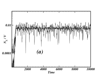
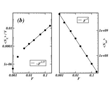
Figure 3: Local interactions. (a): the normalized number of languages $N_{L}/V$ plotted versus simulation time steps. These data indicate that $N_{L}$ increases linearly with $V$. Parameter values are $I=10^{6}$, $F=0.1$ and different $V$ values between $10000$ and $10^{7}$. (b): Averaged total population size $<N_{Tot}>$ and the normalized averaged number of languages $<N_{L}>/V$ versus the fragmentation probability $F$ ($I=10^{6}$).

In Fig. 3b, we show the power law dependence of the total population size and of the number of languages with the parameter $F$, which controls the fragmentation process.

Figure 4a shows the shape of the DPL for different values of the parameter $V$ and of the interaction strength $I$. It is possible to obtain a data collapse by rescaling the distribution with the value of $V$ and the population size with the factor $V/I$. It is interesting to note that, in log-scale, the broadness of the distribution does not depend on $V$ or $I$. As can be clearly observed, the shape of the curve deviates strongly from a lognormal shape for small and large population values. In fact, we collected data over sufficiently many decades to be able to show that the curves decay like a power law for small and large population sizes.

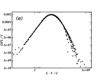
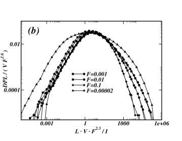
Figure 4: Local interactions. (a): Histogram collapse for different $I$ and $V$. Apparently, the shape is not lognormal but a combination of two power laws. The parameter ranges for the 17 simulations are $I=10^{3}-10^{8}$ and $V=10^{4}-10^{7}$. $F$ is fixed and equals $0.1$. (b): Rescaled histogram for different values of the fragmentation probability $F$. The F-scaling in the horizontal axis is introduced in order to collapse the position of the maxima for different simulations. The parameter ranges are $I=10^{3}-10^{7}$, different values of $V$ and $F=2\cdot 10^{-5}-0.1$. The smaller $F$, the broader is the distribution.

Figure 4b shows the shape of the distribution for different values of all parameters of the model. The fragmentation probability $F$ changes the width of the distributions. For smaller $F$ we obtain broader distributions. From the analysis of this data we obtain scaling relations for the maximum value of the distribution (scaling with $VF^{2.3}/I$) and for its normalization ($VF^{1.6}$). This last scaling relation follows exactly from the $V$ and $F$ dependence on the averaged number of languages, $N_{L}$, shown in Fig. 3b.

Using these scaling relations we can estimate the parameters values for running a simulation that can reproduce the DPL of real data. In fact, these parameters correspond to the ones that allow the rescaling of the DPL of real data to collapse with the ones shown in Fig 4b. Taking $F=2\cdot 10^{-5}$ from adjusting the broadness of the distribution, the values of the others parameters are $I=1.5\cdot 10^{3}$, $V=5\cdot 10^{11}$. Unfortunately, these values correspond to simulations with too demanding computational time. For this reason, we are forced to just test the quality of the collapse of rescaled real data and the rescaled simulation, and we can not do a direct comparison. We carry out a simulation with the parameters $F=2\cdot 10^{-5},I=10^{7}$ and $V=3.2\cdot 10^{12}$. In Fig. 5, we can see how the DPL collapses well with our simulation if we neglect very small population sizes ($L<100$). In addition, our model can reproduce the behavior of the fat tail well (which corresponds to frequently spoken languages).

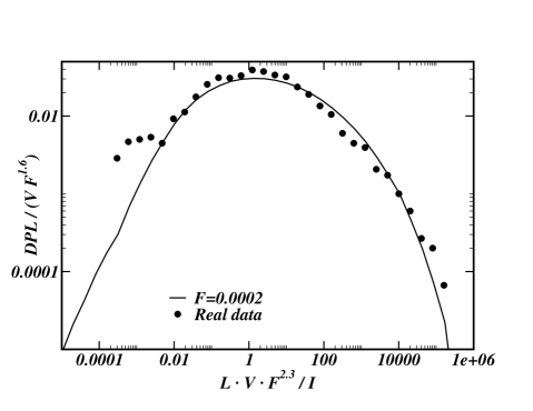
Figure 5: Local interactions. The real data (circles) is rescaled with the values $I=1.5\cdot 10^{3}$, $V=5\cdot 10^{11}$ and $F=2\cdot 10^{-5}$. These parameters correspond to the one that allow rescaling of real data with the ones shown in Fig 4. The continuous line represents the rescaled simulation results. The parameters used in the simulation are: $I=10^{7}$, $V=3.2\cdot 10^{12}$ and $F=2\cdot 10^{-5}$.

Mean field

The increasing connection between people speaking different mother languages suggests exploring the behaviour of our model located on a topology with more links than those of a 1–dimensional array. For this reason, we decided to explore the other limiting situation: a fully connected model (mean field like description). Even if this is a quite unrealistic implementation, we would like to estimate the upper bound for our dynamics, corresponding to a fully globalized world.

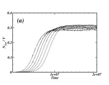
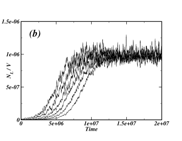
Figure 6: Mean field interactions. The normalized total population (a) and the normalized number of languages (b) versus simulation time steps. We fixed $I=100$ and $F=0.001$ and varied $V$ from $10^{8}$ to $32\cdot 10^{8}$. The figures show that both quantities approximately increase linearly with $V$. For smaller $V$, the stationary state is reached faster.

Figure 6 shows the normalized total population, $N_{Tot}/V$, and the normalized language number, $N_{L}/V$, for different $V$ values. In this topology, both quantities approximately grow linearly with $V$ and $N_{Tot}$ does not reach any saturation value. This novel behavior is due to the different form of carrying out the sum in the second term of Eq. 7. In fact, in this implementation, the sum is taken over all languages and not only over the two neighbors, making the sum to have values of the order of $N_{tot}$.

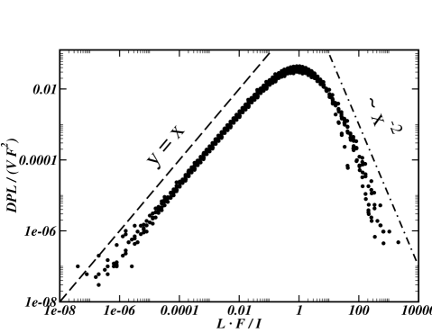
Figure 7: Mean field interactions. Data collapse for the distribution of language size in terms of speaker population. Sufficiently large total populations are considered (large $V$ values). Also for this implementation, the distributions show fat tails, with exponents 1 and -2. The parameter ranges are within $I=10-100,000$, $V=10,000-10^{9}$ and $F=0.001-0.1$.

For large values of $V$, the distribution approaches a fixed lognormal-like shape. In Fig 7, we show the data collapse for different values of the parameters $V$, $I$ and $F$. Surprisingly, the scaling relations are really simple and all DPLs can be perfectly collapsed into each other. On the logarithmic scale, the width of the distribution remains fixed and it does not change when varying the parameters values. Even the $F$-dependence, leading to a different broadness of the DPL in the previous implementation, disappears. The distribution clearly shows two power law decays with exponents $1$ and $-2$.

These results are quite intriguing. On the one hand, the fixed value of the distribution broadness does not allow the reproduction of the real data of actual language sizes. On the other hand, it suggests an interesting conjecture. If the increasing connection between people, in the future, will allow the description of their interaction using a mean field like approximation, our model may provide some predictions. Independently on the population growth, the width of the DPL distribution will get narrower. This means that, despite of the probable growth of the world population, more languages will become extinct than new languages appear. The number of less spoken languages will strongly decrease.

4 Conclusions

A careful analysis of the distribution of population sizes of languages (DPL) suggests that the behavior of its tail is better described by a power law. For this reason, a fit of the real data using the so-called double-Pareto lognormal distribution generates better results than the fit with a pure lognormal distribution.

These deviations from a pure lognormal distribution mean that simple models that reproduce exactly such distributions must be improved. We implemented a new toy model on a 1-dimensional topology that, starting from a macroscopic description at the sub-population level, accounts for two general mechanisms: language competition and fragmentation. These ingredients are sufficient to generate distributions that well reproduce real data, particularly the behavior of frequently spoken languages (the right tail of the distribution).

Moreover, we studied our model on a fully connected network, in which all sub-populations are in mutual contact (mean field like behavior). This implementation can be a good approximation for describing the trend for the interaction patterns on a future, characterized by more and more interconnected communities. This model version allows a simple prediction that confirms previous conjectures about the future mass extinction of languages [17]: despite of the probable growth of the world’s population, more languages will become extinct than new languages will appear.

Finally, we want to recall that, as our toy model is based on simple and general rules, it may be characteristic for systems other than language evolution as well. In fact, systems with an interplay between a fragmentation process and a size dependent growth should exhibit similar patterns. A good example comes from the description of the growth of companies [32, 33, 34] or from the analysis of the mutual fund size distribution [35]. In these systems it is possible to describe the size distributions in terms of log-normal-like distributions In fact, as a zeroth order approximation, log-normal distributions can naturally be generated by a multiplicative growth processes, in which the company size, at any given time, is given as a multiplicative factor times the size of the company at a previous time. For the logarithm of the company size, this process becomes an additive process and so the distribution converges to a normal distribution, obeying the central limit theorem (Gibrat’s law [36] and theory of breakage [37]). Small variations in this approach, as the introduction of some type of cutoff, can modify the lognormal distribution into a heavy tailed distribution [22]. This is obtained, for example, by introducing creation and annihilation processes [38, 39]. At this level of description, none of the components of the random process depend on size. Anyway, it is well known that the growth rates of companies are size dependent [32, 40, 41] and once size effects are taken into account the predictions for the distribution can become more quantitative [35]. This description of the growth of companies is similar to our approach, in the sense that the dynamics of creation and annihilation in growing phenomena can be analogously described introducing the process of fragmentation as well as its counterpart, the phenomenon of coalescence. Our work points out the importance of taking into account these mechanisms, in modelling systems usually described in terms of birth and death processes or random growth [42].

References

References

- [1] L. L. Cavalli-Sforza. Genes, peoples and languages. Proc. Natl. Acad. Sci., 94:7719–7724, 1997.
- [2] L. L. Cavalli-Sforza. Genes, peoples and languages. Penguin, London, 2001.
- [3] J. Maynard Smith and E. Szathmary. The Major Transitions in Evolution. Freeman Spektrum, Oxford, 1995.
- [4] D. M. Abrams and S. H. Strogatz. Modelling the dynamics of language death. Nature, 424:900, 2003.
- [5] M. Patriarca and T. Leppänen. Modeling language competition. Physica A, 338:296–299, 2004.
- [6] J. Mira and A. Paredes. Interlinguistic similarity and language death dynamics. Europh. Lett., 69:1031–1034, 2005.
- [7] K. Kosmidis, J. M Halley, and P. Argyrakis. Language evolution and population dynamics in a system of two interacting species. Physica A, 353:595–612, 2005.
- [8] C. Schulze and D. Stauffer. Monte Carlo simulation of the rise and the fall of languages. Int. J. Mod. Phys. C, 16:781, 2005.
- [9] D. Stauffer and C. Schulze. Microscopic and macroscopic simulation of competition between languages. Physics of Life Reviews, 2:89–116, 2005.
- [10] V. Schwämmle. Simulation for competition of languages with an ageing sexual population. Int. J. Mod. Phys. C, 16:1519–1526, 2005.
- [11] J. P. Pinasco and L. Romanelli. Physica A, 355:355, 2006.
- [12] V. de Oliveira, M. A. F. Gomes, and I. R. Tsang. Theoretical model for the evolution of the linguistic diversity. Physica A, 361:361–370, 2006.
- [13] D. Stauffer, S. Moss de Oliveira, P. M. C. de Oliveira, and J. S. Sá Martins. Biology, Sociology, Geology by Computational Physicists. Elsevier, Amsterdam, 2006.
- [14] C. Schulze, D. Stauffer, and S. Wichmann. Birth, survival and death of languages by monte carlo simulation. Comm. Comp. Phys., 3:371–394, 2008. arxiv:0704.0691.
- [15] M. I. Sereno. Four analogies between biological and cultural/linguistic evolution. J. Theor. Biol., 151:467–507, 1991.
- [16] B. Spagnolo, D. Valenti, and A. Fiasconaro. Noise in ecosystems: A short review. Math. Biosci. Eng., 1:185–211, 2004.
- [17] W. J. Sutherland. Parallel extinction risk and global distribution of languages and species. Nature, 423:276–279, 2003.
- [18] P. A. Stephens and W. J. Sutherland. Trends Ecol. Evol., 14:401, 1999.
- [19] B. F. Grimes. Ethnologue: languages of the world. Summer Institute of Linguistics, Dallas, TX, 14 edition, 2000. www.sil.org.
- [20] Ç. Tuncay. Int. J. Mod. Phys. C, 19:471, 2008.
- [21] D. H. Zanette. Int. J. Mod. Phys. C, 19:237, 2008.
- [22] M Mitzenmacher. A brief history of generative models for power law and lognormal di stributions. Internet Math., 1:226, 2004.
- [23] M Mitzenmacher. Dynamic models for file sizes and double pareto distributions. Internet Math., 1:305, 2004.
- [24] P. M. C. de Oliveira, D. Stauffer, F. W. S. Lima, A. O. Sousa, C. Schulze, and S. Moss de Oliveira. Physica A, 376:609, 2007.
- [25] P. M. C. de Oliveira, D. Stauffer, S. Wichmann, and S. Moss de Oliveira. J. Linguistics, 44:659, 2008.
- [26] V. Schwämmle and P. M. C. de Oliveira. A simple branching model that reproduces language family and language population distributions. Physica A, 388(14):2874 – 2879, 2009.
- [27] M. A. F. Gomes, G. L. Vasconcelos, I. J. Tsang, and I. R Tsang. Scaling relations for diversity of languages. Physica A, 271:489 – 495, 1999.
- [28] W. J. Reed and B. D. Hughes. On the size distribution of live genera. J. Theor. Biol., 217:129, 2002.
- [29] W. J. Reed and M. Jorgensen. The double pareto-lognormal distribution - a new parametric model for size distribution. Comm. Statist. - Theor. Meth., 33:1733, 2004.
- [30] H. Akaike. A new look at the statistical model identification. IEEE Trans. Automat. Contr. AC, 19:716, 1974.
- [31] R. Delannay, G. Le Caër, and R. Botet. J. Phys. A, 29:6693, 1996.
- [32] M. H. R. Stanley, L. A. N. Amaral, S. V. Buldyrev, S. Havlin, H. Leschhorn, P. Maass, M. A. Salinger, and H. E. Stanley. Nature, 379:804, 1996.
- [33] L. A. N. Amaral, S. V. Buldyrev, S. Havlin, M. A. Salinger, and H. E. Stanley. Phys. Rev. Lett., 80:1385, 1998.
- [34] Y. Lee, L. A. N. Amaral, D. Canning, M. Martin Meyer, and H. E. Stanley. Phys. Rev. Lett., 81:3275, 1998.
- [35] Y. Schwarzkopf and J. D. Farmer. Time evolution of the mutual fund size distribution. 2008.
- [36] R. Gibrat. Les inegalites economiques. Libraire du Recueil Sirey, Paris, 1931.
- [37] A. N. Kolmogorov. Dokl. Akad. Nauk SSSR, 30:9, 1941.
- [38] H. A. Simon and C. P. Bonini. The size distribution of business firms. The American Economic Review, 48:607–617, 1958.
- [39] V. Plerou X. Gabaix, P. Gopikrishnan and H.E. Stanley. A theory of power-law distributions in financial market fluctuations. Nature, 423:267–270, 2003.
- [40] M. H. R. Stanley, S. V. Buldyrev, S. Havlin, R. N. Mantegna, M. A. Salinger, and H. E. Stanley. Zipf plots and the size distribution of firms. Economics Letters, 49:453–457, 1995.
- [41] G. Bottazzi and A. Secchi. Common properties and sectoral specificities in the dynamics of U.S. manufacturing companies. Review of Industrial Organization, 23:217–232, 2003.
- [42] A. Saichev, Y. Malevergne, and D. Sornette. Theory of Zipf’s law and of general power law distributions with Gibrat’s law of proportional growth. arxiv:0808.1828, book to be published, 2008.