LHC Phenomenology for Physics Hunters

Abstract

Welcome to the 2008 TASI lectures on the exciting topic of ‘tools and technicalities’ (original title). Technically, LHC physics is really all about perturbative QCD in signals or backgrounds. Whenever we look for interesting signatures at the LHC we get killed by QCD. Therefore, I will focus on QCD issues which arise for example in Higgs searches or exotics searches at the LHC, and ways to tackle them nowadays. In the last section you will find a few phenomenological discussions, for example on missing energy or helicity amplitudes.

I LHC Phenomenology

When we think about signal or background processes at the LHC the first quantity we compute is the total number of events we would expect at the LHC in a given time interval. This number of events is the product of the hadronic (i.e.  proton–proton) LHC luminosity measured in inverse femtobarns and the total production cross section measured in femtobarns. A typical year of LHC running could deliver around 10 inverse femtobarns per year in the first few years and three to ten times that later. People who build the actual collider do not use these kinds of units, but for phenomenologists they work better than something involving seconds and square meters, because what we typically need is a few interesting events corresponding to a few femtobarns of data. So here are a few key numbers and their orders of magnitude for typical signals:

$$N_{\rm events}=\sigma_{\rm tot}\cdot\mathcal{L}\qquad\quad\mathcal{L}=10\cdots 300\,\text{fb}^{-1}\qquad\quad\sigma_{\rm tot}=1\cdots 10^{4}\,\text{fb}$$ (1)

Just in case my colleagues have not told you about it: there are two kinds of processes at the LHC. The first involves all particles which we know and love, like old-fashioned electrons or slightly more modern $W$ and $Z$ bosons or most recently top quarks. These processes we call backgrounds and find annoying. They are described by QCD, which means QCD is the theory of the evil. Top quarks have an interesting history, because when I was a graduate student they still belonged to the second class of processes, the signals. These typically involve particles we have not seen before. Such states are unfortunately mostly produced in QCD processes as well, so QCD is not entirely evil. If we see such signals, someone gets a call from Stockholm, shakes hands with the king of Sweden, and the corresponding processes instantly turn into backgrounds.

The main problem at any collider is that signals are much more rare that background, so we have to dig our signal events out of a much larger number of background events. This is what most of this lecture will be about. Just to give you a rough idea, have a look at Fig. 1: at the LHC the production cross section for two bottom quarks at the LHC is larger than $10^{5}$ nb or $10^{11}$ fb and the typical production cross section for $W$ or $Z$ boson ranges around 200 nb or $2\times 10^{8}$ fb. Looking at signals, the production cross sections for a pair of 500 GeV gluinos is $4\times 10^{4}$ fb and the Higgs production cross section can be as big as $2\times 10^{5}$ fb. When we want to extract such signals out of comparably huge backgrounds we need to describe these backgrounds with an incredible precision. Strictly speaking, this holds at least for those background events which populate the signal region in phase space. Such background event will always exist, so any LHC measurement will always be a statistics exercise. The high energy community has therefore agreed that we call a five sigma excess over the known backgrounds a signal:

$$\frac{S}{\sqrt{B}} =N_{\sigma}>5\qquad\qquad\qquad$$ (Gaussian limit)

$$P_{\rm fluct} <5.8\times 10^{-7}$$ (fluctuation probability) (2)

Do not trust anybody who wants to sell you a three sigma evidence as a discovery, even I have seen a great number of those go away. People often have good personal reasons to advertize such effects, but all they are really saying is that their errors do not allow them to make a conclusive statement. This brings us to a well kept secret in the phenomenology community, which is the important impact of error bars when we search for exciting new physics. Since for theorists understanding LHC events and in particular background events means QCD, we need to understand where our predictions come from and what they assume, so here we go…

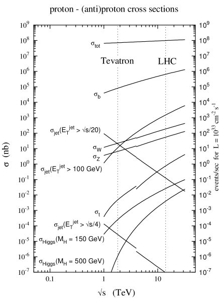
Figure 1: Production rates for different signal and background processes at hadron colliders. The discontinuity is due to the Tevatron being a proton–antiproton collider while the LHC is a proton–proton collider. The two colliders correspond to the $x$–axis values of 2 TeV and 14 TeV. Figure borrowed from CMS.

II QCD and scales

Not all processes which involve QCD have to look incredibly complicated — let us start with a simple question: we know how to compute the production rate and distributions for $Z$ production for example at LEP $e^{+}e^{-}\to Z$. To make all phase space integrals simple, we assume that the $Z$ boson is on-shell, so we can simply add a decay matrix element and a decay phase space integration for example compute the process $e^{+}e^{-}\to Z\to\mu^{+}\mu^{-}$.

So here is the question: how do we compute the production of a $Z$ boson at the LHC? This process is usually referred to as Drell–Yan production, even though we will most likely produce neither Drell nor Yan at the LHC. In our first attempts we explicitly do not care about additional jets, so if we assume the proton consists of quarks and gluons we simply compute the process $q\bar{q}\to Z$ under the assumption that the quarks are partons inside protons. Modulo the $SU(2)$ and $U(1)$ charges which describe the $Zf\bar{f}$ coupling

$$-i\gamma^{\mu}\left(\ell P_{L}+rP_{R}\right)\qquad\qquad\ell=\frac{e}{s_{w}c_{w}}\;\left(T_{3}-Qs_{w}^{2}\right)\qquad\quad r=\ell\Big{|}_{T_{3}=0}$$ (3)

the matrix element and the squared matrix element for the partonic process $q\bar{q}\to Z$ will be the same as the corresponding matrix element squared for $e^{+}e^{-}\to Z$, with an additional color factor. This color factor counts the number of $SU(3)$ states which can be combined to form a color singlet like the $Z$. This additional factor should come out of the color trace which is part of the Feynman rules, and it is $N_{c}$. On the other hand, we do not observe color in the initial state, and the color structure of the incoming $q\bar{q}$ pair has no impact on the $Z$–production matrix element, so we average over the color. This gives us another factor $1/N_{c}^{2}$ in the averaged matrix element (modulo factors two)

$$\overline{|\mathcal{M}|^{2}}(q\bar{q}\to Z)\sim\frac{1}{4N_{c}}\;m_{Z}^{2}\;\left(\ell^{2}+r^{2}\right)\,.$$ (4)

Notice that matrix elements we compute from our Feynman rules are not automatically numbers without a mass unit. Next, we add the phase space for a one-particle final state. In four space–time dimensions (this will become important later) we can compute a total cross section out of a matrix element squared as

$$s\;\frac{d\sigma}{dy} =\frac{\pi}{(4\pi)^{2}}\;\left(1-\tau\right)\;\overline{|\mathcal{M}|^{2}}$$

The mass of the final state appears as $\tau=m_{Z}^{2}/s$ and can of course be $m_{W}$ or the Higgs mass or the mass of a KK graviton (I know you smart-asses in the back row!). If we define $s$ as the partonic invariant mass of the two quarks using the Mandelstam variable $s=(k_{2}+k_{2})^{2}=2(k_{1}k_{2})$, momentum conservation just means $s=m_{Z}^{2}$. This simple one-particle phase space has only one free parameter, the reduced polar angle $y=(1+\cos\theta)/2=0\cdots 1$. The azimuthal angle $\phi$ plays no role at colliders, unless you want to compute gravitational effects on Higgs production at Atlas and CMS. Any LHC Monte Carlo will either random-generate a reference angle $\phi$ for the partonic process or pick one and keep it fixed. The second option has at least once lead to considerable confusion and later amusement at the Tevatron, when people noticed that the behavior of gauge bosons was dominated by gravity, namely gauge bosons going up or down. So this is not as trivial a statement as you might think. At this point I remember that every teacher at every summer schools always feels the need to define their field of phenomenology — for example: phenomenologists are theorists who do useful things and know funny stories about experiment(alist)s.

Until now we have computed the same thing as $Z$ production at LEP, leaving open the question how to describe quarks inside the proton. For a proper discussion I refer to any good QCD textbook and in particular the chapter on deep inelastic scattering. Instead, I will follow a pedagogical approach which will as fast as possible take us to the questions we really want to discuss.

If for now we are happy assuming that quarks move collinear with the surrounding proton, i.e.  that at the LHC incoming partons have zero $p_{T}$, we can simply write a probability distribution for finding a parton with a certain fraction of the proton’s momentum. For a momentum fraction $x=0\cdots 1$ this parton density function (pdf) is denoted as $f_{i}(x)$, where $i$ describes the different partons in the proton, for our purposes $u,d,c,s,g$. All of these partons we assume to be massless. We can talk about heavy bottoms in the proton if you ask me about it later. Note that in contrast to structure functions a pdf is not an observable, it is simply a distribution in the mathematical sense, which means it has to produce reasonably results when integrated over as an integration kernel. These parton densities have very different behavior — for the valence quarks ($uud$) they peak somewhere around $x\lesssim 1/3$, while the gluon pdf is small at $x\sim 1$ and grows very rapidly towards small $x$. For some typical part of the relevant parameter space ($x=10^{-3}\cdots 10^{-1}$) you can roughly think of it as $f_{g}(x)\propto x^{-2}$, towards $x$ values it becomes even steeper. This steep gluon distribution was initially not expected and means that for small enough $x$ LHC processes will dominantly be gluon fusion processes.

Given the correct definition and normalization of the pdf we can compute the hadronic cross section from its partonic counterpart as

$$\sigma_{\rm tot}=\int_{0}^{1}dx_{1}\int_{0}^{1}dx_{2}\;f_{i}(x_{1})\,f_{j}(x_{2})\;\hat{\sigma}_{ij}(x_{1}x_{2}S)$$ (6)

where $i,j$ are the incoming partons with the momentum factions $x_{i,j}$. The partonic energy of the scattering process is $s=x_{1}x_{2}S$ with the LHC proton energy $\sqrt{S}=14$ TeV. The partonic cross section $\hat{\sigma}$ corresponds to the cross sections $\sigma$ we already discussed. It has to include all the necessary $\Theta$ and $\delta$ functions for energy–momentum conservation. When we express a general $n$–particle cross section $\hat{\sigma}$ including the phase space integration, the $x_{i}$ integrations and the phase space integrations can of course be swapped, but Jacobians will make your life hell when you attempt to get them right. Luckily, there are very efficient numerical phase space generators on the market which transform a hadronic $n$–particle phase space integration into a unit hypercube, so we do not have to worry in our every day life.

II.1 UV divergences and the renormalization scale

Renormalization, i.e.  the proper treatment of ultraviolet divergences, is one of the most important aspects of field theories; if you are not comfortable with it you might want to attend a lecture on field theory. The one aspect of renormalization I would like to discuss is the appearance of the renormalization scale. In perturbation theory, scales arise from the regularization of infrared or ultraviolet divergences, as we can see writing down a simple loop integral corresponding to two virtual massive scalars with a momentum $p$ flowing through the diagram:

$$B(p^{2};m,m)\equiv\int\frac{d^{4}q}{16\pi^{2}}\;\frac{1}{q^{2}-m^{2}}\frac{1}{(q+p)^{2}-m^{2}}$$ (7)

Such diagrams appear for example in the gluon self energy, with massless scalars for ghosts, with some Dirac trace in the numerator for quarks, and with massive scalars for supersymmetric scalar quarks. This integral is UV divergent, so we have to regularize it, express the divergence in some well-defined manner, and get rid of it by renormalization. One way is to introduce a cutoff into the momentum integral $\Lambda$, for example through the so-called Pauli–Villars regularization. Because the UV behavior of the integrand cannot depend on IR-relevant parameters, the UV divergence cannot involve the mass $m$ or the external momentum $p^{2}$. This means that its divergence has to be proportional to $\log\Lambda/\mu^{2}$ with some scale $\mu^{2}$ which is an artifact of the regularization of such a Feynman diagram.

This question is easier to answer in the more modern dimensional regularization. There, we shift the power of the momentum integration and use analytic continuation in the number of space–time dimensions to renormalize the theory

$$\int\frac{d^{4}q}{16\pi^{2}}\cdots\longrightarrow\mu^{2\epsilon}\;\int\frac{d^{4-2\epsilon}q}{16\pi^{2}}\cdots=\frac{i\mu^{2\epsilon}}{(4\pi)^{2}}\;\left[\frac{C_{-1}}{\epsilon}+C_{0}+C_{1}\,\epsilon+\mathcal{O}(\epsilon^{2})\right]$$ (8)

The constants $C_{i}$ depend on the loop integral we are considering. The scale $\mu$ we have to introduce to ensure the matrix element and the observables, like cross sections, have the usual mass dimensions. To regularize the UV divergence we pick an $\epsilon>0$, giving us mathematically well-defined poles $1/\epsilon$. If you compute the scalar loop integrals you will see that defining them with the integration measure $1/(i\pi^{2})$ will make them come out as of the order $\mathcal{O}(1)$, in case you ever wondered about factors $1/(4\pi)^{2}=\pi^{2}/(2\pi)^{4}$ which usually end up in front of the loop integrals.

The poles in $\epsilon$ will cancel with the counter terms, i.e.  we renormalize the theory. Counter terms we include by shifting the renormalized parameter in the leading-order matrix element, e.g.  $\overline{|\mathcal{M}|^{2}}(g)\to\overline{|\mathcal{M}|^{2}}(g+\delta g)$ with a coupling $\delta g\propto 1/\epsilon$, when computing $|\mathcal{M}_{\rm Born}+\mathcal{M}_{\rm virt}|^{2}$. If we use a physical renormalization condition there will not be any free scale $\mu$ in the definition of $\delta g$. As an example for a physical reference we can think of the electromagnetic coupling or charge $e$, which is usually defined in the Thomson limit of vanishing momentum flow through the diagram, i.e.  $p^{2}\to 0$. What is important about these counter terms is that they do not come with a factor $\mu^{2\epsilon}$ in front.

So while after renormalization the poles $1/\epsilon$ cancel just fine, the scale factor $\mu^{2\epsilon}$ will not be matched between the UV divergence and the counter term. We can keep track of it by writing a Taylor series in $\epsilon$ for the prefactor of the regularized but not yet renormalized integral:

$$\mu^{2\epsilon}\;\left[\frac{C_{-1}}{\epsilon}+C_{0}+\mathcal{O}(\epsilon)\right] =e^{2\epsilon\log\mu}\;\left[\frac{C_{-1}}{\epsilon}+C_{0}+\mathcal{O}(\epsilon)\right]$$

$$=\left[1+2\epsilon\log\mu+\mathcal{O}(\epsilon^{2})\right]\;\left[\frac{C_{-1}}{\epsilon}+C_{0}+\mathcal{O}(\epsilon)\right]$$

$$=\frac{C_{-1}}{\epsilon}+C_{0}+2\log\mu\,C_{-1}+\mathcal{O}(\epsilon)$$ (9)

We see that the pole $C_{-1}/\epsilon$ gives a finite contribution to the cross section, involving the renormalization scale $\mu_{R}\equiv\mu$.

Just a side remark for completeness: from eq.(9) we see that we should not have just pulled out $\mu^{2\epsilon}$ out of the integral, because it leads to a logarithm of a number with a mass unit. On the other hand, from the way we split the original integral we know that the remaining $(4-2\epsilon)$-dimensional integral has to includes logarithms of the kind $\log m^{2}$ or $\log p^{2}$ which re-combine with the $\log\mu^{2}$ for example to a properly defined $\log\mu/m$. The only loop integral which has no intrinsic mass scale is the two-point function with zero mass in the loop and zero momentum flowing through the integral: $B(p^{2}=0;0,0)$. It appears for example as a self-energy correction of external quarks and gluons. Based on these dimensional arguments this integral has to be zero, but with a subtle cancellation of the UV and the IR divergences which we can schematically write as $1/\epsilon_{\rm IR}-1/\epsilon_{\rm UV}$. Actually, I am thinking right now if following this argument this integral has to be zero or if it can still be a number, like 2376123/67523, but it definitely has to be finite… And it is zero if you compute it.

Instead of discussing different renormalization schemes and their scale dependences, let us instead compute a simple renormalization scale dependent parameter, namely the running strong coupling $\alpha_{s}(\mu_{R})$. It does not appear in our Drell–Yan process at leading order, but it does not hurt to know how it appears in QCD calculations. The simplest process we can look at is two-jet production at the LHC, where we remember that in some energy range we will be gluon dominated: $gg\to q\bar{q}$. The Feynman diagrams include an $s$–channel off-shell gluon with a momentum flow $p^{2}\equiv s$. At next-to-leading order, this gluon propagator will be corrected by self-energy loops, where the gluon splits into two quarks or gluons and re-combines before it produces the two final-state partons.

The gluon self energy correction (or vacuum polarization, as propagator corrections to gauge bosons are often labelled) will be a scalar, i.e.  fermion loops will be closed and the Dirac trace is closed inside the loop. In color space the self energy will (hopefully) be diagonal, just like the gluon propagator itself, so we can ignore the color indices for now. In Minkowski space the gluon propagator in unitary gauge is proportional to the transverse tensor $T^{\mu\nu}=g^{\mu\nu}-p^{\nu}p^{\mu}/p^{2}$. The same is true for the gluon self energy, which we write as $\Pi^{\mu\nu}\equiv\Pi\,T^{\mu\nu}$. The one useful thing to remember is the simple relation $T^{\mu\nu}T_{\nu}^{\rho}=T^{\mu\rho}$ and $T^{\mu\nu}g_{\nu}^{\rho}=T^{\mu\rho}$. Including the gluon, quark, and ghost loops the regularized gluon self energy with a momentum flow $p^{2}$ reads

$$\frac{1}{p^{2}}\;\Pi\left(\frac{\mu_{R}^{2}}{p^{2}}\right) = \frac{\alpha_{s}}{4\pi}\;\left(-\frac{1}{\epsilon}-\log\frac{\mu_{R}^{2}}{p^{2}}\right)\;\left(\frac{13}{6}N_{c}-\frac{2}{3}n_{f}\right)+\mathcal{O}(\log m_{t}^{2})$$

$$\longrightarrow\; \frac{\alpha_{s}}{4\pi}\;\left(-\frac{1}{\epsilon}-\log\frac{\mu_{R}^{2}}{p^{2}}\right)\;\beta_{g}+\mathcal{O}(\log m_{t}^{2})$$

$$\text{with}\qquad\beta_{g}=\frac{11}{3}N_{c}-\frac{2}{3}n_{f}\,.$$ (10)

In the second step we have sneaked in additional contributions to the renormalization of the strong coupling from the other one-loop diagrams in the process. The number of fermions coupling to the gluons is $n_{f}$. We neglect the additional terms $\log(4\pi)$ and $\log\gamma_{E}$ which come with the poles in dimensional regularization. From the comments on the function $B(p^{2};0,0)$ before we could have guessed that the loop integrals will only give a logarithm $\log p^{2}$ which then combines with the scale logarithm $\log\mu_{R}^{2}$. The finite top mass actually leads to an additional logarithms which we omit for now — this zero-mass limit of our field theory is actually special and referred to as its conformal limit.

Lacking a well-enough motivated reference point (in the Thomson limit the strong coupling is divergent, which means QCD is confined towards large distances and asymptotically free at small distances) we are tempted to renormalize $\alpha_{s}$ by also absorbing the scale into the counter term, which is called the $\overline{\rm MS}$ scheme. It gives us a running coupling $\alpha_{s}(p)$. In other words, for a given momentum transfer $p^{2}$ we cancel the UV pole and at the same time shift the strong coupling, after including all relative ($-$) signs, by

$$\alpha_{s}\longrightarrow\alpha_{s}(\mu_{R}^{2})\;\left(1-\frac{1}{p^{2}}\;\Pi\left(\frac{\mu_{R}^{2}}{p^{2}}\right)\right)=\alpha_{s}(\mu_{R}^{2})\;\left(1-\frac{\alpha_{s}}{4\pi}\;\beta_{g}\;\log\frac{p^{2}}{\mu_{R}^{2}}\right)\,.$$ (11)

We can do even better: the problem with the correction to $\alpha_{s}$ is that while it is perturbatively suppressed by the usual factor $\alpha_{s}/(4\pi)$ it includes a logarithm which does not need to be small. Instead of simply including these gluon self-energy corrections at a given order in perturbation theory we can instead include all chains with $\Pi$ appearing many times in the off-shell gluon propagator. Such a series means we replace the off-shell gluon propagator by (schematically written)

$$\frac{T^{\mu\nu}}{p^{2}}\longrightarrow \frac{T^{\mu\nu}}{p^{2}}+\left(\frac{T}{p^{2}}\cdot(-T\,\Pi)\cdot\frac{T}{p^{2}}\right)^{\mu\nu}$$

$$\hskip 20.0pt+\left(\frac{T}{p^{2}}\cdot(-T\,\Pi)\cdot\frac{T}{p^{2}}\cdot(-T\,\Pi)\cdot\frac{T}{p^{2}}\right)^{\mu\nu}+\cdots$$

$$= \;\frac{T^{\mu\nu}}{p^{2}}\;\sum_{j=0}^{\infty}\left(-\frac{\Pi}{p^{2}}\right)^{j}=\frac{T^{\mu\nu}}{p^{2}}\;\frac{1}{1+\Pi/p^{2}}$$ (12)

To avoid indices we abbreviate $T^{\mu\nu}T_{\nu}^{\rho}=T\cdot T$ which can be simplified using $(T\cdot T\cdot T)^{\mu\nu}=T^{\mu\rho}T^{\sigma}_{\rho}T_{\sigma}^{\nu}=T^{\mu\nu}$. This re-summation of the logarithm which occurs in the next-to-leading order corrections to $\alpha_{s}$ moves the finite shift in $\alpha_{s}$ shown in eq.(11) into the denominator:

$$\alpha_{s}\longrightarrow\alpha_{s}(\mu_{R}^{2})\;\left(1+\frac{\alpha_{s}}{4\pi}\;\beta_{g}\;\log\frac{p^{2}}{\mu_{R}^{2}}\right)^{-1}$$ (13)

If we interpret the renormalization scale $\mu_{R}$ as one reference point $p_{0}$ and $p$ as another, we can relate the values of $\alpha_{s}$ between two reference points with a renormalization group equation (RGE) which evolves physical parameters from one scale to another:

$$\alpha_{s}(p^{2}) =\alpha_{s}(p_{0}^{2})\;\left(1+\frac{\alpha_{s}(p_{0}^{2})}{4\pi}\;\beta_{g}\;\log\frac{p^{2}}{p_{0}^{2}}\right)^{-1}$$

$$\frac{1}{\alpha_{s}(p^{2})} =\frac{1}{\alpha_{s}(p_{0}^{2})}\left(1+\frac{\alpha_{s}(p_{0}^{2})}{4\pi}\;\beta_{g}\;\log\frac{p^{2}}{p_{0}^{2}}\right)=\frac{1}{\alpha_{s}(p_{0}^{2})}+\frac{1}{4\pi}\;\beta_{g}\;\log\frac{p^{2}}{p_{0}^{2}}$$ (14)

The factor $\alpha_{s}$ inside the parentheses can be evaluated at any of the two scales, the difference is going to be a higher-order effect. The interpretation of $\beta_{g}$ is now obvious: when we differentiate the shifted $\alpha_{s}(p^{2})$ with respect to the momentum transfer $p^{2}$ we find:

$$\frac{1}{\alpha_{s}}\;\frac{d\alpha_{s}}{d\log p^{2}}=-\frac{\alpha_{s}}{4\pi}\beta_{g}\qquad\qquad\text{or}\qquad\qquad\frac{1}{g_{s}}\;\frac{dg_{s}}{d\log p}=-\frac{\alpha_{s}}{4\pi}\beta_{g}=-g_{s}^{2}\beta_{g}$$ (15)

This is the famous running of the strong coupling constant!

Before we move on, let us collect the logic of the argument given in this section: when we regularize an UV divergence we automatically introduce a reference scale. Naively, this could be a UV cutoff scale, but even the seemingly scale invariant dimensional regularization cannot avoid the introduction of a scale, even in the conformal limit of our theory. There are several ways of dealing with such a scale: first, we can renormalize our parameter at a reference point. Secondly, we can define a running parameter, i.e.  absorb the scale logarithm into the $\overline{\rm MS}$ counter term. This way, at each order in perturbation theory we can translate values for example of the strong coupling from one momentum scale to another momentum scale. If we are lucky, we can re-sum these logarithms to all orders in perturbation theory, which gives us more precise perturbative predictions even in the presence of large logarithms, i.e.  large scale differences for our renormalized parameters. Such a (re–) summation is linked with the definition of scale dependent parameters.

II.2 IR divergences and the factorization scale

After this brief excursion into renormalization and UV divergences we can return to the original example, the Drell–Yan process at the LHC. In our last attempt we wrote down the hadronic cross sections in terms of parton distributions at leading order. These pdfs are only functions of the (collinear) momentum fraction of the partons in the proton.

The perturbative question we need to ask for this process is: what happens if we radiate additional jets which for one reason or another we do not observe in the detector. Throughout this writeup I will use the terms jets and final state partons synonymously, which is not really correct once we include jet algorithms and hadronization. On the other hand, in most cases a jet algorithms is designed to take us from some kind of energy deposition in the calorimeter to the parton radiated in the hard process. This is particularly true for modern developments like the so-called matrix element method to measure the top mass. Recently, people have looked into the question what kind of jets come from very fast collimated $W$ or top decays and how such fat jets could be identified looking into the details of the jet algorithm. But let’s face it, you can try to do such analyses after you really understand the QCD of hard processes, and you should not trust such analyses unless they come from groups which know a whole lot of QCD and preferable involve experimentalists who know their calorimeters very well.

So let us get back to the radiation of additional partons in the Drell–Yan process. These can for example be gluons radiated from the incoming quarks. This means we can start by compute the cross section for the partonic process $q\bar{q}\to Zg$. However, this partonic process involves renormalization as well as an avalanche of loop diagrams which have to be included before we can say anything reasonable, i.e.  UV and IR finite. Instead, we can look at the crossed process $qg\to Zq$, which should behave similarly as a $2\to 2$ process, except that it has a different incoming state than the leading-order Drell–Yan process and hence no virtual corrections. This means we do not have to deal with renormalization and UV divergences and can concentrate on parton or jet radiation from the initial state.

The amplitude for this $2\to 2$ process is — modulo the charges and averaging factors, but including all Mandelstam variables

$$\overline{|\mathcal{M}|^{2}}\propto 8\left[-\frac{t}{s}-\frac{s}{t}+\frac{2m_{Z}^{2}(s+t-m_{Z}^{2})}{st}\right]$$ (16)

The new Mandelstam variables can be expressed in terms of the rescaled gluon-emission angle $y=(1+\cos\theta)/2$ as $t=-s(1-\tau)y$ and $u=-s(1-\tau)(1-y)$. As a sanity check we can confirm that $t+u=-s+m_{Z}^{2}$. The collinear limit when the gluon is radiated in the beam direction is given by $y\to 0$, which corresponds to $t\to 0$ with finite $u=-s+m_{Z}^{2}$. In that case the matrix element becomes

$$\overline{|\mathcal{M}|^{2}}\sim 8\left[\frac{s^{2}-2sm_{Z}^{2}+2m_{Z}^{4}}{s(s-m_{Z}^{2})}\;\frac{1}{y}-\frac{2m_{Z}^{2}}{s}\;+\mathcal{O}(y)\right]$$ (17)

This expression is divergent for collinear gluon radiation, i.e.  for small angles $y$. We can translate this $1/y$ divergence for example into the transverse momentum of the gluon or $Z$ according to

$$sp_{T}^{2}=tu=s^{2}(1-\tau)^{2}\;y(1-y)=(s-m_{Z}^{2})^{2}y+\mathcal{O}(y^{2})$$ (18)

In the collinear limit our matrix element squared then becomes

$$\overline{|\mathcal{M}|^{2}}\sim 8\left[\frac{s^{2}-2sm_{Z}^{2}+2m_{Z}^{4}}{s^{2}}\;\frac{(s-m_{Z}^{2})}{p_{T}^{2}}+\mathcal{O}(p_{T}^{0})\right]\,.$$ (19)

The matrix element for the tree-level process $qg\to Zq$ diverges like $1/p_{T}^{2}$. To compute the total cross section for this process we need to integrate it over the two-particle phase space. Without deriving this result we quote that this integration can be written in the transverse momentum of the outgoing particles, in which case the Jacobian for this integration introduces a factor $p_{T}$. Approximating the matrix element as $C/p_{T}^{2}$, we have to integrate

$$\int_{y^{\rm min}}^{y^{\rm max}}dy\frac{C}{y}=\int_{p_{T}^{\rm min}}^{p_{T}^{\rm max}}dp_{T}^{2}\frac{C}{p_{T}^{2}}= \;2\int_{p_{T}^{\rm min}}^{p_{T}^{\rm max}}dp_{T}\;p_{T}\;\frac{C}{p_{T}^{2}}$$

$$\simeq \;2C\int_{p_{T}^{\rm min}}^{p_{T}^{\rm max}}dp_{T}\frac{1}{p_{T}}=2C\;\log\frac{p_{T}^{\rm max}}{p_{T}^{\rm min}}$$ (20)

The form $C/p_{T}^{2}$ for the matrix element is of course only valid in the collinear limit; in the remaining phase space $C$ is not a constant. However, this formula describes well the collinear IR divergence arising from gluon radiation at the LHC (or photon radiation at $e^{+}e^{-}$ colliders, for that matter).

We can follow the same strategy as for the UV divergence. First, we regularize the divergence using dimensional regularization, and then we find a well-defined way to get rid of it. Dimensional regularization now means we have to write the two-particle phase space in $n=4-2\epsilon$ dimensions. Just for the fun, here is the complete formula in terms of $y$:

$$s\;\frac{d\sigma}{dy}=\frac{\pi(4\pi)^{-2+\epsilon}}{\Gamma(1-\epsilon)}\;\left(\frac{\mu^{2}}{m_{Z}^{2}}\right)^{\epsilon}\;\frac{\tau^{\epsilon}(1-\tau)^{1-2\epsilon}}{y^{\epsilon}(1-y)^{\epsilon}}\overline{|\mathcal{M}|^{2}}\sim\left(\frac{\mu^{2}}{m_{Z}^{2}}\right)^{\epsilon}\;\frac{\overline{|\mathcal{M}|^{2}}}{y^{\epsilon}(1-y)^{\epsilon}}\,.$$ (21)

In the second step we only keep the factors we are interested in. The additional factor $y^{-\epsilon}$ regularizes the integral at $y\to 0$, as long as $\epsilon<0$, which just slightly increases the suppression of the integrand in the IR regime. After integrating the leading term $1/y^{1+\epsilon}$ we have a pole $1/(-\epsilon)$. Obviously, this regularization procedure is symmetric in $y\leftrightarrow(1-y)$. What is important to notice is again the appearance of a scale $\mu^{2\epsilon}$ with the $n$-dimensional integral. This scale arises from the IR regularization of the phase space integral and is referred to as factorization scale $\mu_{F}$.

From our argument we can safely guess that the same divergence which we encounter for the process $qg\to Zq$ will also appear in the crossed process $q\bar{q}\to Zg$, after cancelling additional soft IR divergences between virtual and real gluon emission diagrams. We can write all these collinear divergences in a universal form, which is independent of the hard process (like Drell–Yan production). In the collinear limit, the probabilities of radiating additional partons or splitting into additional partons is given by universal splitting functions, which govern the collinear behavior of the parton-radiation cross section:

$$\frac{1}{\sigma_{\rm tot}}\;d\sigma\sim\frac{\alpha_{s}}{2\pi}\;\frac{dy}{y}\;dx\;P_{j}(x)=\frac{\alpha_{s}}{2\pi}\;\frac{dp_{T}^{2}}{p_{T}^{2}}\;dx\;P_{j}(x)$$ (22)

The momentum fraction which the incoming parton transfers to the parton entering the hard process is given by $x$. The rescaled angle $y$ is one way to integrate over the transverse-momentum space. The splitting kernels are different for different partons involved:

$$P_{q\leftarrow q}(x) =C_{F}\;\frac{1+x^{2}}{1-x}\qquad\qquad\qquad P_{g\leftarrow q}(x)=C_{F}\;\frac{1+(1-x)^{2}}{x}$$

$$P_{q\leftarrow g}(x) =T_{R}\;\left(x^{2}+(1-x)^{2}\right)$$

$$P_{g\leftarrow g}(x) =C_{A}\;\left(\frac{x}{1-x}+\frac{1-x}{x}+x(1-x)\right)$$ (23)

The underlying QCD vertices in these four collinear splittings are the $qqg$ and $ggg$ vertices. This means that a gluon can split independently into a pair of quarks and a pair of gluons. A quark can only radiate a gluon, which implies $P_{q\leftarrow q}(1-x)=P_{g\leftarrow q}(x)$, depending on which of the two final state partons we are interested in. For these formulas we have sneaked in the Casimir factors of $SU(N)$, which allow us to generalize our approach beyond QCD. For practical purposes we can insert the SU(3) values $C_{F}=(N_{c}^{2}-1)/(2N_{c})=4/3$, $C_{A}=N_{c}=3$ and $T_{R}=1/2$. Once more looking at the different splitting kernels we see that in the soft-daughter limit $x\to 0$ the daughter quarks $P_{q\leftarrow q}$ and $P_{q\leftarrow g}$ are well defined, while the gluon daughters $P_{g\leftarrow q}$ and $P_{g\leftarrow g}$ are infrared divergent.

What we need for our partonic subprocess $qg\to Zq$ is the splitting of a gluon into two quarks, one of which then enters the hard Drell–Yan process. In the collinear limit this splitting is described by $P_{q\leftarrow g}$. We explicitly see that there is no additional soft singularity for vanishing quark energy, only the collinear singularity in $y$ or $p_{T}$. This is good news, since in the absence of virtual corrections we would have no idea how to get rid of or cancel this soft divergence.

Figure 2: Feynman diagrams for the repeated emission of a gluon from the incoming leg of a Drell–Yan process. The labels indicate the appearance of $\alpha_{s}$ as well as the leading divergence of the phase space integration.

If we for example consider repeated collinear gluon emission off an incoming quark leg, we naively get a correction suppressed by powers of $\alpha_{s}$, because of the strong coupling of the gluon. Such a chain of gluon emissions is illustrated in Fig. 2. On the other hand, the $y$ integration over each new final state gluon combined with the $1/y$ or $1/p_{T}$ divergence in the matrix element squared leads to a possibly large logarithm which can be easiest written in terms of the upper and lower boundary of the $p_{T}$ integration. This means, at higher orders we expect corrections of the form

$$\sigma_{\rm tot}\sim\sum_{j}C_{j}\;\left(\alpha_{s}\log\frac{p_{T}^{\rm max}}{p_{T}^{\rm min}}\right)^{j}$$ (24)

with some factors $C_{j}$. Because the splitting probability is universal, these fixed-order corrections can be re-summed to all orders, just like the gluon self energy. You notice how successful perturbation theory becomes every time we encounter a geometric series? And again, in complete analogy with the gluon self energy, this universal factor can be absorbed into another quantity, which are the parton densities.

However, there are three important differences to the running coupling:

First, we are now absorbing IR divergences into running parton densities. We are not renormalizing them, because renormalization is a well-defined procedure to absorb UV divergences into a redefined Lagrangian.

Secondly, the quarks and gluons split into each other, which means that the parton densities will form a set of coupled differential equations which describe their running instead of a simple differential equation with a beta function.

And third, the splitting kernels are not just functions to multiply the parton densities, but they are integration kernels, so we end up with a coupled set of integro-differential equations which describe the parton densities as a function of the factorization scale. These equation are called the Dokshitzer–Gribov–Lipatov–Altarelli–Parisi or DGLAP equations

$$\frac{df_{i}(x,\mu_{F})}{d\log\mu_{F}^{2}}=\frac{\alpha_{s}}{2\pi}\;\sum_{j}\;\int_{x}^{1}\;\frac{dx^{\prime}}{x^{\prime}}\;P_{i\leftarrow j}\left(\frac{x}{x^{\prime}}\right)\;f_{j}(x^{\prime},\mu_{F})\,.$$ (25)

We can discuss this formula briefly: to compute the scale dependence of a parton density $f_{i}$ we have to consider all partons $j$ which can split into $i$. For each splitting process, we have to integrate over all momentum fractions $x^{\prime}$ which can lead to a momentum fraction $x$ after splitting, which means we have to integrate $z$ from $x$ to 1. The relative momentum fraction in the splitting is then $x/z<1$.

The DGLAP equation by construction resums collinear logarithms. There is another class of logarithms which can potentially become large, namely soft logarithms $\log x$, corresponding to the soft divergence of the diagonal splitting kernels. This reflects the fact that if you have for example a charged particle propagating there are two ways to radiate photons without any cost in probability, either collinear photons or soft photons. We know from QED that both of these effects lead to finite survival probabilities once we sum up these collinear and soft logarithms. Unfortunately, or fortunately, we have not seen any experimental evidence of these soft logarithms dominating the parton densities yet, so we can for now stick to DGLAP.

Going back to our original problem, we can now write the hadronic cross section production for Drell–Yan production or other LHC processes as:

$$\sigma_{\rm tot}(\mu_{F},\mu_{R})=\int_{0}^{1}dx_{1}\int_{0}^{1}dx_{2}\;f_{i}(x_{1},\mu_{F})\,f_{j}(x_{2},\mu_{F})\;\hat{\sigma}_{ij}(x_{1}x_{2}S,\mu_{R})$$ (26)

Since our particular Drell–Yan process at leading order only involves weak couplings, it does not include $\alpha_{s}$ at leading order. We will only see $\alpha_{s}$ and with it a renormalization scale $\mu_{R}$ appear at next-to-leading order, when we include an additional final state parton.

After this derivation, we can attempt a physical interpretation of the factorization scale. The collinear divergence we encounter for example in the $qg\to Zq$ process is absorbed into the parton densities using the universal collinear splitting kernels. In other words, as long as the $p_{T}$ distribution of the matrix element follows eq.(20), the radiation of any number of additional partons from the incoming partons is now included. These additional partons or jets we obviously cannot veto without getting into perturbative hell with QCD. This is why we should really write $pp\to Z+X$ when talking about factorization-scale dependent parton densities as defined in eq.(26).

If we look at the $d\sigma/dp_{T}$ distribution of additional partons we can divide the entire phase space into two regions. The collinear region is defined by the leading $1/p_{T}$ behavior. At some point the $p_{T}$ distribution will then start decreasing faster, for example because of phase space limitations. The transition scale should roughly be the factorization scale. In the DGLAP evolution we approximate all parton radiation as being collinear with the hadron, i.e.  move them from the region $p_{T}<\mu_{F}$ onto the point $p_{T}=0$. This kind of $p_{T}$ spectrum can be nicely studied using bottom parton densities. They have the advantage that there is no intrinsic bottom content in the proton. Instead, all bottoms have to arise from gluon splitting, which we can compute using perturbative QCD. If we actually compute the bottom parton densities, the factorization scale is not an unphysical free parameter, but it should at least roughly come out of the calculation of the bottom parton densities. So we can for example compute the bottom-induced process $b\bar{b}\to H$ including resummed collinear logarithms using bottom densities or derive it from the fixed-order process $gg\to b\bar{b}H$. When comparing the $p_{T,b}$ spectra it turns out that the bottom factorization scale is indeed proportional to the Higgs mass (or hard scale), but including a relative factor of the order $1/4$. If we naively use $\mu_{F}=m_{H}$ we will create an inconsistency in the definition of the bottom parton densities which leads to large higher-order corrections.

Going back to the $p_{T}$ spectrum of radiated partons or jets — when the transverse momentum of an additional parton becomes large enough that the matrix element does not behave like eq.(20) anymore, this parton is not well described by the collinear parton densities. We should definitely choose $\mu_{F}$ such that this high-$p_{T}$ range is not governed by the DGLAP equation. We actually have to compute the hard and now finite matrix elements for $pp\to Z+$jets to predict the behavior of these jets. How to combine collinear jets as they are included in the parton densities and hard partonic jets is what the rest of this lecture will be about.

	renormalization scale $\mu_{R}$	factorization scale $\mu_{F}$
source	ultraviolet divergence	collinear (infrared) divergence
poles cancelled	counter terms	parton densities
	(renormalization)	(mass factorization)
summation	resum self energy bubbles	resum collinear logarithms
parameter	running coupling $\alpha_{s}(\mu_{R})$	parton density $f_{j}(x,\mu_{F})$
evolution	RGE for $\alpha_{s}$	DGLAP equation
large scales	typically decrease of $\sigma_{\rm tot}$	typically increase of $\sigma_{\rm tot}$
theory	renormalizability	factorization
	proven for gauge theories	proven all order for DIS
		proven order-by-order DY…

Table 1: Comparison of renormalization and factorization scales appearing in LHC cross sections.

II.3 Right or wrong scales

Looking back at the last two sections we introduce the factorization and renormalization scales completely in parallel. First, computing perturbative higher-order contributions to scattering amplitudes we encounter divergences. Both of them we regularize, for example using dimensional regularization (remember that we had to choose $n=4-2\epsilon<4$ for UV and $n>4$ for IR divergences). After absorbing the divergences into a re-definition of the respective parameters, referred to as renormalization for example of the strong coupling in the case of an UV divergence and as mass factorization absorbing IR divergences into the parton distributions we are left with a scale artifact. In both cases, this redefinition was not perturbative at fixed order, but involved summing possibly large logarithms. The evolution of these parameters from one renormalization/factorization scale to another is described either by a simple beta function in the case of renormalization and by the DGLAP equation in the case of mass factorization. There is one formal difference between these two otherwise very similar approaches. The fact that we can actually absorb UV divergences into process-independent universal counter terms is called renormalizability and has been proven to all orders for the kind of gauge theories we are dealing with. The universality of IR splitting kernels has not (yet) in general been proven, but on the other hand we have never seen an example where is failed. Actually, for a while we thought there might be a problem with factorization in supersymmetric theories using the supersymmetric version of the $\overline{\rm MS}$ scheme, but this has since been resolved. A comparison of the two relevant scales for LHC physics is shown in Tab. 1

The way I introduced factorization and renormalization scales clearly describes an artifact of perturbation theory and the way we have to treat divergences. What actually happens if we include all orders in perturbation theory? In that case for example the resummation of the self-energy bubbles is simply one class of diagrams which have to be included, either order-by-order or rearranged into a resummation. For example the two jet production rate will then not depend on arbitrarily chosen renormalization or factorization scales $\mu$. Within the expression for the cross section, though, we know from the arguments above that we have to evaluate renormalized parameters at some scale. This scale dependence will cancel once we put together all its implicit and explicit appearances contributing to the total rate at all orders. In other words, whatever scale we evaluate the strong couplings at gets compensated by other scale logarithms in the complete expression. In the ideal case, these logarithms are small and do not spoil perturbation theory by inducing large logarithms. If we think of a process with one distinct external scale, like the $Z$ mass, we know that all these logarithms have the form $\log\mu/m_{Z}$. This logarithm is truly an artifact, because it would not need to appear if we evaluated everything at the ‘correct’ external energy scale of the process, namely $m_{Z}$. In that sense we can even think of the running coupling as an running observable, which depends on the external energy of the process. This energy scale is not a perturbative artifact, but the cross section even to all orders really depends on the external energy scale. The only problem is that most processes after analysis cuts have more than one scale.

We can turn this argument around and estimate the minimum theory error on a prediction of a cross section to be given by the scale dependence in an interval around what we would consider a reasonable scale. Notice that this error estimate is not at all conservative; for example the renormalization scale dependence of the Drell–Yan production rate is zero, because $\alpha_{s}$ only enters are next-to-leading order. At the same time we know that the next-to-leading order correction to the cross section at the LHC is of the order of 30%, which far exceeds the factorization scale dependence.

Guessing the right scale choice for a process is also hard. For example in leading-order Drell–Yan production there is one scale, $m_{Z}$, so any scale logarithm (as described above) has to be $\log\mu/m_{Z}$. If we set $\mu=m_{Z}$ all scale logarithms will vanish. In reality, any observable at the LHC will include several different scales, which do not allow us to just define just one ‘correct’ scale. On the other hand, there are definitely completely wrong scale choices. For example, using $1000\times m_{Z}$ as a typical scale in the Drell–Yan process will if nothing else lead to logarithms of the size $\log 1000$ whenever a scale logarithm appears. These logarithms have to be cancelled to all orders in perturbation theory, introducing unreasonably large higher-order corrections.

When describing jet radiation, people usually introduce a phase-space dependent renormalization scale, evaluating $\alpha_{s}(p_{T,j})$. This choice gives the best kinematic distributions for the additional partons, but to compute a cross section it is the one scale choice which is forbidden by QCD and factorization: scales can only depend on exclusive observables, i.e.  momenta which are given after integrating over the phase space. For the Drell–Yan process such a scale could be $m_{Z}$, or the mass of heavy new-physics states in their production process. Otherwise we double-count logarithms and spoil the collinear resummation. But as long as we are mostly concerned with distributions, we even use the transverse-momentum scale very successfully. To summarize this brief mess: while there is no such thing as the correct scale choice, there are more or less smart choices, and there are definitely very wrong choices, which lead to an unstable perturbative behavior.

Of course, these sections on divergences and scales cannot do the topic justice. They fall short left and right, hardly any of the factors are correct (they are not that important either), and I am omitting any formal derivation of this resummation technique for the parton densities. On the other hand, we can derive some general message from them: because we compute cross sections in perturbation theory, the absorption of ubiquitous UV and IR divergences automatically lead to the appearance of scales. These scales are actually useful because running parameters allow us to resum logarithms in perturbation theory, or in other words allow us to compute certain dominant effects to all orders in perturbation theory, in spite of only computing the hard processes at a given loop order. This means that any LHC observable we compute will depend on the factorization and renormalization scales, and we have to learn how to either get rid of the scale dependence by having the Germans compute higher and higher loop orders, or use the Californian/Italian approach to derive useful scale choices in a relaxed atmosphere, to make use of the resummed precision of our calculation.

III Hard vs collinear jets

Jets are a major problem we are facing at the Tevatron and will be the most dangerous problem at the LHC. Let’s face it, the LHC is not built do study QCD effects. To the contrary, if we wanted to study QCD, the Tevatron with its lower luminosity would be the better place to do so. Jets at the LHC by themselves are not interesting, they are a nuisance and they are the most serious threat to the success of the LHC program.

The main difference between QCD at the Tevatron and QCD at the LHC is the energy scale of the jets we encounter. Collinear jets or jets with a small transverse momentum, are well described by partons in the collinear approximation and simulated by a parton shower. This parton shower is the attempt to undo the approximation $p_{T}\to 0$ we need to make when we absorb collinear radiation in parton distributions using the DGLAP equation. Strictly speaking, the parton shower can and should only fill the phase space region $p_{T}=0...\mu_{F}$ which is not covered by explicit additional parton radiation. Such so-called hard jets or jets with a large transverse momentum are described by hard matrix elements which we can compute using the QCD Feynman rules. Because of the logarithmic enhancement we have observed for collinear additional partons, there are much more collinear and soft jets than hard jets.

The problem at the LHC is the range of ‘soft’ or ‘collinear’ and ‘hard’. As mentioned above, we can define these terms by the validity of the collinear approximation in eq.(20). The maximum $p_{T}$ of a collinear jet is the region for which the jet radiation cross section behaves like $1/p_{T}$. We know that for harder and harder jets we will at some point become limited by the partonic energy available at the LHC, which means the $p_{T}$ distribution of additional jets will start dropping faster than $1/p_{T}$. At this point the logarithmic enhancement will cease to exist, and jets will be described by the regular matrix element squared without any resummation.

Quarks and gluons produced in association with gauge bosons at the Tevatron behave like collinear jets for $p_{T}\lesssim 20$ GeV, because the quarks at the Tevatron are limited in energy. At the LHC, jets produced in association with tops behave like collinear jets to $p_{T}\sim 150$ GeV, jets produced with 500 GeV gluinos behave like collinear jets to $p_{T}$ scales larger than 300 GeV. This is not good news, because collinear jets means many jets, and many jets produce combinatorical backgrounds or ruin the missing momentum resolution of the detector. Maybe I should sketch the notion of combinatorical backgrounds: if you are looking for example for two jets to reconstruct an invariant mass you can simply plot all events as a function of this invariant mass and cut the background by requiring all event to sit around a peak in $m_{jj}$. However, if you have for example three jets in the event you have to decide which of the three jet-jet combinations should go into this distribution. If this seems not possible, you can alternatively consider two of the three combinations as uncorrelated ‘background’ events. In other words, you make three histogram entries out of your signal or background event and consider all background events plus two of the three signal combinations as background. This way the signal-to-background ratio decreases from $N_{S}/N_{B}$ to $N_{S}/(3N_{B}+2N_{S})$, i.e.  by at least a factor of three. You can guess that picking two particles out of four candidates with its six combinations has great potential to make your analysis a candidate for this circular folder under your desk. The most famous victim of such combinatorics might be the formerly promising Higgs discovery channel $pp\to t\bar{t}H$ with $H\to b\bar{b}$.

All this means for theorists that at the LHC we have to learn how to model collinear and hard jets reliably. This is what the remainder of the QCD lectures will be about. Achieving this understanding I consider the most important development in QCD since I started working on physics. Discussing the different approaches we will see why such general–$p_{T}$ jets are hard to understand and even harder to properly simulate.

III.1 Sudakov factors

Before we discuss any physics it makes sense to introduce the so-called Sudakov factors which will appear in the next sections. This technical term is used by QCD experts to ensure that other LHC physicists feel inferior and do not get on their nerves. But, really, Sudakov factors are nothing but simple survival probabilities. Let us start with an event which we would expect to occur $p$ times, given its probability and given the number of shots. The probability of observing it $n$ times is given by the Poisson distribution

$$\mathcal{P}(n;p)=\frac{p^{n}\,e^{-p}}{n!}\,.$$ (27)

This distribution will develop a mean at $p$, which means most of the time we will indeed see about the expected number of events. For large numbers it will become a Gaussian. In the opposite direction, using this distribution we can compute the probability of observing zero events, which is $\mathcal{P}(0;p)=e^{-p}$. This formula comes in handy when we want to know how likely it is that we do not see a parton splitting in a certain energy range.

According to the last section, the differential probability of a parton to split or emit another parton at a scale $\mu$ and with the daughter’s momentum fraction $x$ is given by the splitting kernel $P_{i\leftarrow j}(x)$ times $dp_{T}^{2}/p_{T}^{2}$. This energy measure is a little tricky because we compute the splitting kernels in the collinear approximation, so $p_{T}^{2}$ is the most inconvenient observable to use. We can approximately replace the transverse momentum by the virtuality $Q$, to get to the standard parameterization of parton splitting — I know I am just waving my hands at this stage, to understand the more fundamental role of the virtuality we would have to look into deep inelastic scattering and factorization. In terms of the virtuality, the splitting of one parton into two is given by the splitting kernel integrated over the proper range in the momentum fraction $x$

$$d\mathcal{P}(x) =\frac{\alpha_{s}}{2\pi}\;\frac{dq^{2}}{q^{2}}\;\int\;dx\;P(x)$$

$$\mathcal{P}(Q_{\rm min},Q_{\rm max}) =\frac{\alpha_{s}}{2\pi}\;\int_{Q_{\rm min}}^{Q_{\rm max}}\;\frac{dq^{2}}{q^{2}}\;\int_{x_{\rm min}}^{x_{\rm max}}\;dx\;P(x)$$ (28)

The splitting kernel we symbolically write as $P(x)$, avoiding indices and the sum over partons appearing in the DGLAP equation eq.(25). The boundaries $x_{\rm min}$ and $x_{\rm max}$ we can compute for example in terms of an over-all minimum value $Q_{0}$ and the actual values $q$, so we drop them for now. Strictly speaking, the double integral over $x$ and $q^{2}$ can lead to two overlapping IR divergences or logarithms, a soft logarithm arising from the $x$ integration (which we will not discuss further) and the collinear logarithm arising from the virtuality integral. This is the logarithm we are interested in when talking about the parton shower.

In the expression above we compute the probability that a parton will split into another parton while moving from a virtuality $Q_{\rm max}$ down to $Q_{\rm min}$. This probability is given by QCD, as described earlier. Using it, we can ask what the probability is that we will not see a parton splitting from a parton starting at fixed $Q_{\rm max}$ to a variable scale $Q$, which is precisely the Sudakov factor

$$\Delta(Q,Q_{\rm max}) =e^{-\mathcal{P}(Q,Q_{\rm max})}$$

$$=\exp\left[-\frac{\alpha_{s}}{2\pi}\int_{Q}^{Q_{\rm max}}\;\frac{dq^{2}}{q^{2}}\;\int_{x_{\rm min}}^{x_{\rm max}}\;dx\;P(x)\right]\sim e^{-\alpha_{s}\log^{2}Q_{\rm max}/Q}$$ (29)

The last line omits all kinds of factors, but correctly identifies the logarithms involved, namely $\alpha_{s}^{n}\log^{2n}Q_{\rm max}/Q$.

III.2 Jet algorithm

Before discussing methods to describe jets at the LHC we should introduce one way to define jets in a detector, namely the $k_{T}$ jet algorithm. Imagine we observe a large number of energy depositions in the calorimeter in the detector which we would like to combine into jets. We know that they come from a smaller number of partons which originate in the hard QCD process and which since have undergone a sizeable number of splittings. Can we try to reconstruct partons?

The answer is yes, in the sense that we can combine a large number of jets into smaller numbers, where unfortunately nothing tells us what the final number of jets should be. This makes sense, because in QCD we can produce an arbitrary number of hard jets in a hard matrix element and another arbitrary number via collinear radiation. The main difference between a hard jet and a jet from parton splitting is that the latter will have a partner which originated from the same soft or collinear splitting.

The basic idea of the $k_{T}$ algorithm is to ask if a given jet has a soft or collinear partner. For this we have to define a collinearity measure, which will be something like the transverse momentum of one jet with respect to another one $y_{ij}\sim k_{T,ij}$. If one of the two jets is the beam direction, this measure simply becomes $y_{iB}\sim k_{T,i}$. We define two jets as collinear, if $y_{ij}<y_{\rm cut}$ where $y_{\rm cut}$ we have to give to the algorithm. The jet algorithm is simple:

• for all final state jets find minimum $y^{\rm min}={\rm min}_{ij}(y_{ij},y_{iB})$

• if $y^{\rm min}=y_{ij}<y_{\rm cut}$ merge jets $i$ and $j$, go back to (1)

• if $y^{\rm min}=y_{iB}<y_{\rm cut}$ remove jet $i$, go back to (1)

• if $y^{\rm min}>y_{\rm cut}$ keep all jets, done

The result of the algorithm will of course depend on the resolution $y_{\rm cut}$. Alternatively, we can just give the algorithm the minimum number of jets and stop there. The only question is what ‘combine jets’ means in terms of the 4-momentum of the new jet. The simplest thing would be to just combine the momentum vectors $k_{i}+k_{j}\to k_{i}$, but we can still either combine the 3-momenta and give the new jet a zero invariant mass (which assumes it indeed was one parton) or we can add the 4-momenta and get a jet mass (which means they can come from a $Z$, for example). But these are details for most new-physics searches at the LHC. At this stage we run into a language issue: what do we really call a jet? I am avoiding this issue by saying that jet algorithms definitely start from calorimeter towers and not jets and then move more and more towards jets, where likely the last iterations could be described by combining jets into new jets.

From the QCD discussion above it is obvious why theorists prefer a $k_{T}$ algorithm over for other algorithms which define the distance between two jets in a more geometric manner: a jet algorithm combines the complicated energy deposition in the hadronic calorimeter, and we know that the showering probability or theoretically speaking the collinear splitting probability is best described in terms of virtuality or transverse momentum. A transverse-momentum distance between jets is from a theory point of view best suited to combine the right jets into the original parton from the hard interaction. Moreover, this $k_{T}$ measure is intrinsically infrared safe, which means the radiation of an additional soft parton cannot affect the global structure of the reconstructed jets. For other algorithms we have to ensure this property explicitly, and you can find examples for this in QCD lectures by Mike Seymour.

One problem of the $k_{T}$ algorithm is that noise and the underlying event can easiest be understood geometrically in the $4\pi$ detector. Basically, the low-energy jet activity is constant all over the detector, so the easiest thing to do is just subtract it from each event. How much energy deposit we have to subtract from a reconstructed jet depends on the actual area the jet covers in the detector. Therefore, it is a major step for the $k_{T}$ algorithm that it can indeed compute an IR–safe geometric size of the jet. Even more, if this size is considerably smaller than the usual geometric measures, the $k_{T}$ algorithm should at the end of the day turn out to be the best jet algorithm at the LHC.

IV Jet merging

So how does a traditional Monte Carlo treat the radiation of jets into the final state? It needs to reverse the summation of collinear jets done by the DGLAP equation, because jet radiation is not strictly collinear and does hit the detector. In other words, it computes probabilities for radiating collinear jets from other jets and simulates this radiation. Because it was the only thing we knew, Monte Carlos used to do this in the collinear approximation. However, from the brief introduction we know that at the LHC we should generally not use the collinear approximation, which is one of the reason why at the LHC we will use all-new Monte Carlos. Two ways how they work we will discuss here.

Apart from the collinear approximation for jet radiation, a second problem with Monte Carlo simulation is that they ‘only do shapes’. In other words, the normalization of the event sample will always be perturbatively poorly defined. The simple reason is that collinear jet radiation starts from a hard process and its production cross section and from then on works with splitting probabilities, but never touches the total cross section it started from.

Historically, people use higher-order cross sections to normalize the total cross section in the Monte Carlo. This is what we call a $K$ factor: $K=\sigma^{\rm improved}/\sigma^{\rm MC}=\sigma^{\rm improved}/\sigma^{\rm LO}$. It is crucial to remember that higher-order cross sections integrate over unobserved additional jets in the final state. So when we normalize the Monte Carlo we assume that we can first integrate over additional jets and obtain $\sigma^{\rm improved}$ and then just normalize the Monte Carlo which puts back these jets in the collinear approximation. Obviously, we should try to do better than that, and there are two ways to improve this traditional Monte Carlo approach.

IV.1 MC@NLO method

When we compute the next-to-leading order correction to a cross section, for example to Drell–Yan production, we consider all contributions of the order $G_{F}\alpha_{s}$. There are three obvious sets of Feynman diagrams we have to square and multiply, namely the Born contribution $q\bar{q}\to Z$, the virtual gluon exchange for example between the incoming quarks, and the real gluon emission $q\bar{q}\to Zg$. Another set of diagrams we should not forget are the crossed channels $qg\to Zq$ and $\bar{q}g\to Z\bar{q}$. Only amplitudes with the same external particles can be squared, so we get the matrix-element-squared contributions

$$|\mathcal{M}_{B}|^{2} \propto G_{F}$$

$$2{\rm Re}\;\mathcal{M}_{V}^{*}\mathcal{M}_{B} \propto G_{F}\alpha_{s}\quad\quad|\mathcal{M}_{Zg}|^{2} \propto G_{F}\alpha_{s}\quad\quad|\mathcal{M}_{Zq}|^{2},|\mathcal{M}_{Z\bar{q}}|^{2}\propto G_{F}\alpha_{s}$$ (30)

Strictly speaking, we should have included the counter terms, which are a modification of $|\mathcal{M}_{B}|^{2}$, shifted by counter terms of the order $\alpha_{s}(1/\epsilon+C)$. These counter terms we add to the interference of Born and virtual gluon diagrams to remove the UV divergences. Luckily, this is not the part of the contributions we want to discuss. IR poles can have two sources, soft and collinear divergences. The first kind is cancelled between virtual gluon exchange and real gluon emission. Again, we are not really interested in them.

What we are interested in are the collinear divergences. They arise from virtual gluon exchange as well as from gluon emission and from gluon splitting in the crossed channels. The collinear limit is described by the splitting kernels eq.(23), and the divergences are absorbed in the re-definition of the parton densities (like an IR pseudo-renormalization).

To present the idea of MC@NLO Bryan Webber uses a nice toy model which I am going to follow in a shortened version. It describes simplified particle radiation off a hard process: the energy of the system before radiation is $x_{s}$ and the energy of the outgoing particle (call it photon or gluon) is $x$, so $x<x_{s}<1$. When we compute next-to-leading order corrections to a hard process, the different contributions (now neglecting crossed channels) are

$$\frac{d\sigma}{dx}\Big{|}_{B}=B\,\delta(x)\quad\quad\frac{d\sigma}{dx}\Big{|}_{V}=\alpha_{s}\left(\frac{B}{2\epsilon}+V\right)\delta(x)\quad\quad\frac{d\sigma}{dx}\Big{|}_{R}=\alpha_{s}\frac{R(x)}{x}\,.\qquad$$ (31)

The constant $B$ describes the Born process and the assumed factorizing poles in the virtual contribution. The coupling constant $\alpha_{s}$ should be extended by factors 2 and $\pi$, or color factors. We immediately see that the integral over $x$ in the real emission rate is logarithmically divergent in the soft limit, similar to the collinear divergences we now know and love. From factorization (i.e.  implying universality of the splitting kernels) we know that in the collinear and soft limits the real emission part has to behave like the Born matrix element $\lim_{x\to 0}R(x)=B$.

The logarithmic IR divergence we extract in dimensional regularization, as we already did for the virtual corrections. The expectation value of any infrared safe observable over the entire phase space is then given by

$$\langle O\rangle=\mu_{F}^{2\epsilon}\int_{0}^{1}\;dx\;\frac{O(x)}{x^{2\epsilon}}\left[\frac{d\sigma}{dx}\Big{|}_{B}+\frac{d\sigma}{dx}\Big{|}_{V}+\frac{d\sigma}{dx}\Big{|}_{R}\right]\,.$$ (32)

Dimensional regularization yields this additional factor $1/x^{2\epsilon}$, which is precisely the factor whose mass unit we cancel introducing the factorization scale $\mu_{F}^{2\epsilon}$. This renormalization scale factor we will casually drop in the following.

When we compute a distribution of for example the energy of one of the heavy particles in the process, we can extract a histogram from of the integral for $\langle O\rangle$ and obtain a normalized distribution. However, to compute such a histogram we have to numerically integrate over $x$, and the individual parts of the integrand are not actually integrable. To cure this problem, we can use the subtraction method to define integrable functions under the $x$ integral. From the real emission contribution we subtract and then add a smartly chosen term:

$$\langle O\rangle_{R}= \int_{0}^{1}\;dx\;\frac{O(x)}{x^{2\epsilon}}\;\frac{d\sigma}{dx}\Big{|}_{R}=\int_{0}^{1}\;dx\;\frac{O(x)}{x^{2\epsilon}}\;\frac{\alpha_{s}R(x)}{x}$$

$$= \alpha_{s}\;B\;O(0)\int_{0}^{1}\;dx\frac{1}{x^{1+2\epsilon}}+\int_{0}^{1}dx\;\left(\frac{\alpha_{s}R(x)O(x)}{x^{1+2\epsilon}}-\frac{\alpha_{s}BO(0)}{x^{1+2\epsilon}}\right)$$

$$= \alpha_{s}\;B\;O(0)\int_{0}^{1}\;dx\frac{1}{x^{1+2\epsilon}}+\alpha_{s}\int_{0}^{1}dx\;\frac{R(x)O(x)-BO(0)}{x^{1+2\epsilon}}$$

$$= -\alpha_{s}\frac{B\;O(0)}{2\epsilon}+\alpha_{s}\int_{0}^{1}dx\;\frac{R(x)O(x)-BO(0)}{x}$$ (33)

In the second integral we take the limit $\epsilon\to 0$ because the asymptotic behavior of $R(x\to 0)$ makes the numerator vanish and hence regularizes this integral without any dimensional regularization required. The first term precisely cancels the (soft) divergence from the virtual correction. We end up with a perfectly finite $x$ integral for all three contributions

$$\langle O\rangle =B\;O(0)+\alpha_{s}V\;O(0)+\alpha_{s}\int_{0}^{1}\;dx\;\frac{R(x)\;O(x)-B\;O(0)}{x}$$

$$=\int_{0}^{1}\;dx\;\left[O(0)\;\left(B+\alpha_{s}V-\alpha_{s}\frac{B}{x}\right)+O(x)\;\alpha_{s}\;\frac{R(x)}{x}\right]$$ (34)

This procedure is one of the standard methods to compute next-to-leading order corrections involving one-loop virtual contributions and the emission of one additional parton. This formula is a little tricky: usually, the Born-type kinematics would come with an explicit factor $\delta(x)$, which in this special case we can omit because of the integration boundaries. We can re-write the same formula in terms of a derivative

$$\frac{d\sigma}{dO}=\int_{0}^{1}\;dx\;\left[I(O)_{\rm LO}\;\left(B+\alpha_{s}V-\alpha_{s}\frac{B}{x}\right)+I(O)_{\rm NLO}\;\alpha_{s}\;\frac{R(x)}{x}\right]$$ (35)

The transfer function $I(O)$ is defined in a way that formally does precisely what we did before: at leading order we evaluate it using the Born kinematics $x=0$ while allowing for a general $x=0\cdots 1$ for the real emission kinematics.

In this calculation we have integrated over the entire phase space of the additional parton. For a hard additional parton or jet everything looks well defined and finite. On the other hand, we cancel an IR divergence in the virtual corrections proportional to a Born-type momentum configuration $\delta(x)$ with another IR divergence which appears after integrating over small but finite values of $x\to 0$. In a histogram in $x$, where we encounter the real-emission divergence at small $x$, this divergence is cancelled by a negative delta distribution right at $x=0$. Obviously, this will not give us a well-behaved distribution. What we would rather want is a way to smear out this pole such that it coincides with the in that range justified collinear approximation and cancels the real emission over the entire low-$x$ range. At the same time it has to leave the hard emission intact and when integrated give the same result as the next-to-leading oder rate. Such a modification will use the emission probability or Sudakov factors. We can define an emission probability of a particle with an energy fraction $z$ as $d\mathcal{P}=\alpha_{s}E(z)/z\,dz$. Note that we have avoided the complicated proper two–dimensional description in favor of this simpler picture just in terms of particle energy fractions.

Let us consider a perfectly fine observable, the radiated photon spectrum as a function of the (external) energy scale $z$. We know what this spectrum has to look like for the two kinematic configurations

$$\frac{d\sigma}{dz}\Big{|}_{\rm LO}=\alpha_{s}\;\frac{BE(z)}{z}\qquad\qquad\frac{d\sigma}{dz}\Big{|}_{\rm NLO}=\alpha_{s}\;\frac{R(z)}{z}$$ (36)

The first term corresponds to parton shower radiation from the Born diagram (at order $\alpha_{s}$), while the second term is the real emission defined above. The transfer functions we would have to include in eq.(35) to arrive at this equation for the observable are

$$I(z,1)\Big{|}_{\rm LO} =\alpha_{s}\;\frac{E(z)}{z}$$

$$I(z,x_{M})\Big{|}_{\rm NLO} =\delta(z-x)+\alpha_{s}\;\frac{E(z)}{z}\;\Theta(x_{M}(x)-z)$$ (37)

The additional second term in the real-radiation transfer function arises from a parton shower acting on the real emission process. It explicitly requires that enough energy has to be available to radiate a photon with an energy $z$, where $x_{M}$ is the energy available at the respective stage of showering, i.e.  $z<x_{M}$.

These transfer functions we can include in eq.(35), which becomes

$$\frac{d\sigma}{dz} =\int_{0}^{1}dx\;\left[I(z,1)\;\left(B+\alpha_{s}V-\alpha_{s}\frac{B}{x}\right)+I(z,x_{M})\;\alpha_{s}\;\frac{R(x)}{x}\right]$$

$$=\int_{0}^{1}dx\;\left[\alpha_{s}\frac{E(z)}{z}\left(B+\alpha_{s}V-\alpha_{s}\frac{B}{x}\right)+\left(\delta(x-z)+\mathcal{O}(\alpha_{s})\right)\;\alpha_{s}\frac{R(x)}{x}\right]$$

$$=\int_{0}^{1}dx\;\left[\alpha_{s}\;\frac{BE(z)}{z}+\alpha_{s}\;\frac{R(z)}{z}\right]+\mathcal{O}(\alpha_{s}^{2})$$

$$=\alpha_{s}\;\frac{BE(z)+R(z)}{z}+\mathcal{O}(\alpha_{s}^{2})$$ (38)

All Born–type contributions proportional to $\delta(z)$ have vanished by definition. This means we should be able to integrate the $z$ distribution to the total cross section $\sigma_{\rm tot}$ with a $z_{\rm min}$ cutoff for consistency. However, the distribution we obtained above has an additional term which spoils this agreement, so we are still missing something.

On the other hand, we also knew we would fall short, because what we described in words about a subtraction term for finite $x$ cancelling the real emission we have not yet included. This means, first we have to add a subtraction term to the real emission which cancels the fixed-order contributions for small $x$ values. Because of factorization we know how to write such a subtraction term using the splitting function, called $E$ in this example:

$$\frac{R(x)}{x}\quad\longrightarrow\quad\frac{R(x)-BE(x)}{x}$$ (39)

To avoid double counting we have to add this parton shower to the Born-type contribution, now in the collinear limit, which leads us to a modified version of eq.(35)

$$\frac{d\sigma}{dO}=\int_{0}^{1}\;dx\;\Bigg{[}\quad I(O,1)\;\left(B+\alpha_{s}V-\frac{\alpha_{s}B}{x}+\frac{\alpha_{s}BE(x)}{x}\right)$$

$$+ I(O,x_{M})\;\alpha_{s}\frac{R(x)-BE(x)}{x}\Bigg{]}$$ (40)

When we again compute the $z$ spectrum to order $\alpha_{s}$ there will be an additional contribution from the Born-type kinematics

$$\frac{d\sigma}{dz} =\int_{0}^{1}\;dx\;\alpha_{s}\;\frac{BE(z)+R(z)}{z}+\mathcal{O}(\alpha_{s}^{2})$$

$$\longrightarrow\int_{0}^{1}\;dx\;\left[\alpha_{s}\;\frac{BE(z)+R(z)}{z}-\alpha_{s}\;\delta(x-z)\;\frac{BE(x)}{x}\right]+\mathcal{O}(\alpha_{s}^{2})$$

$$=\int_{0}^{1}\;dx\;\alpha_{s}\;\frac{BE(z)+R(z)-BE(z)}{z}+\mathcal{O}(\alpha_{s}^{2})$$

$$=\alpha_{s}\;\frac{R(z)}{z}+\mathcal{O}(\alpha_{s}^{2})$$ (41)

which gives us the distribution we expected, without any double counting.

In other words, this scheme implemented in the MC@NLO Monte Carlo describes the hard emission just like a next-to-leading order calculation, including the next-to-leading order normalization. On top of that, it simulates additional collinear particle emissions using the Sudakov factor. This is precisely what the parton shower does. Most importantly, it avoids double counting between the first hard emission and the collinear jets, which means it describes the entire $p_{T}$ range of jet emission for the first and hardest radiated jet consistently. Additional jets, which do not appear in the next-to-leading order calculation are simply added by the parton shower, i.e.  in the collinear approximation. What looked to easy in our toy example is of course much harder in the mean QCD reality, but the general idea is the same: to combine a fixed-order NLO calculation with a parton shower one can think of the parton shower as a contribution which cancels a properly defined subtraction term which we can include as part of the real emission contribution.

IV.2 CKKW method

The one weakness of the MC@NLO method is that it only describes one hard jet properly and relies on a parton shower and its collinear approximation to simulate the remaining jets. Following the general rule that there is no such thing as a free lunch we can improve on the number of correctly described jets, which unfortunately will cost us the next-to-leading order normalization.

For simplicity, we will limit our discussion to final state radiation, for example in the inverse Drell–Yan process $e^{+}e^{-}\to q\bar{q}$. We know already that this final state is likely to evolve into more than two jets. First, we can radiate a gluon off one of the quark legs, which gives us a $q\bar{q}g$ final state, provided our $k_{T}$ algorithm finds $y_{ij}>y_{\rm cut}$. Additional splittings can also give us any number of jets, and it is not clear how we can combine these different channels.

Each of these processes can be described either using matrix elements or using a parton shower, where ‘describe’ means for example compute the relative probability of different phase space configurations. The parton shower will do well for jets which are fairly collinear, $y_{ij}<y_{\rm ini}$. In contrast, if for our closest jets we find $y_{ij}>y_{\rm ini}$, we know that collinear logarithms did not play a major role, so we can and should use the hard matrix element. How do we combine these two approaches?

The CKKW scheme tackles this multi-jet problem. It first allows us to combine final states with a different number of jets, and then ensures that we can add a parton shower without any double counting. The only thing I will never understand is that they labelled the transition scale as ‘ini’.

Using Sudakov factors we can first construct the probabilities of generating $n$–jet events from a hard two–jet production process. These probabilities make no assumptions on how we compute the actual kinematics of the jet radiation, i.e.  if we model collinear jets with a parton shower or hard jets with a matrix element. This way we will also get a rough idea how Sudakov factors work in practice. For the two–jet and three–jet final states, we will see that we only have to consider the splitting probabilities for the different partons

$$\Gamma_{q}(Q_{\rm out},Q_{\rm in}) \equiv\Gamma_{q\leftarrow q}(Q_{\rm out},Q_{\rm in})=\frac{2C_{F}}{\pi}\;\frac{\alpha_{s}(Q_{\rm out})}{Q_{\rm out}}\;\left(\log\frac{Q_{\rm in}}{Q_{\rm out}}-\frac{3}{4}\right)$$

$$\Gamma_{g}(Q_{\rm out},Q_{\rm in}) \equiv\Gamma_{g\leftarrow q}(Q_{\rm out},Q_{\rm in})=\frac{2C_{A}}{\pi}\;\frac{\alpha_{s}(Q_{\rm out})}{Q_{\rm out}}\;\left(\log\frac{Q_{\rm in}}{Q_{\rm out}}-\frac{11}{12}\right)$$ (42)

The virtualities $Q_{\rm in,out}$ correspond to the incoming (mother) and outgoing (daughter) parton. Unfortunately, this formula is somewhat understandable from the argument before and from $P_{q\leftarrow q}$, but not quite. That has to do with the fact that these splittings are not only collinearly divergent, but also softly divergent, as we can see in the limits $x\to 0$ and $x\to 1$ in eq.(23). These divergences we have to subtract first, so the formulas for the splitting probabilities $\Gamma_{q,g}$ look unfamiliar. In addition, we find finite terms arising from next-to-leading logarithms which spoil the limit $Q_{\rm out}\to Q_{\rm in}$, where the probability of no splitting should go to unity. But at least we can see the leading (collinear) logarithm $\log Q_{\rm in}/Q_{\rm out}$. Technically, we can deal with the finite terms in the Sudakov factors by requiring them to be positive semi-definite, i.e.  by replacing $\Gamma(Q_{\rm out},Q_{\rm in})<0$ by zero.

Given the splitting probabilities we can write down the Sudakov factor, which is the probability of not radiating any hard and collinear gluon between the two virtualities:

$$\Delta_{q,g}(Q_{\rm out},Q_{\rm in})=\exp\left[-\int_{Q_{\rm out}}^{Q_{\rm in}}\;dq\;\Gamma_{q,g}(q,Q_{\rm in})\right]$$ (43)

This integral boundaries are $Q_{\rm out}<Q_{\rm in}$. This description we can generalize for all splittings $P_{i\leftarrow j}$ we wrote down before.

First, we can compute the probability that we see exactly two partons, which means that none of the two quarks radiate a resolved gluon between the virtualities $Q_{2}$ and $Q_{1}$, where we assume that $Q_{1}<Q_{2}$ gives the scale for this resolution. It is simply $\left[\Delta_{q}(Q_{1},Q_{2})\right]^{2}$, once for each quark, so that was easy.

Next, what is the probability that the two–jet final state evolves exactly into three partons? We know that it contains a factor $\Delta_{q}(Q_{1},Q_{2})$ for one untouched quark. If we label the point of splitting in the matrix element $Q_{q}$ for the quark, there has to be a probability for the second quark to get from $Q_{2}$ to $Q_{q}$ untouched, but we leave this to later. After splitting with the probability $\Gamma_{q}(Q_{2},Q_{q})$, this quark has to survive to $Q_{1}$, so we have a factor $\Delta_{q}(Q_{1},Q_{q})$. Let’s call the virtuality of the radiated gluon after splitting $Q_{g}$, then we find the gluon’s survival probability $\Delta_{g}(Q_{1},Q_{g})$. So what we have until now is

$$\Delta_{q}(Q_{1},Q_{2})\;\Gamma_{q}(Q_{2},Q_{q})\;\Delta_{q}(Q_{1},Q_{q})\;\Delta_{g}(Q_{1},Q_{g})\cdots$$ (44)

That’s all there is, with the exception of the intermediate quark. Naively, we would guess its survival probability between $Q_{2}$ and $Q_{q}$ to be $\Delta_{q}(Q_{q},Q_{2})$, but that is not correct. That would imply no splittings resolved at $Q_{q}$, but what we really mean is no splitting resolved later at $Q_{1}<Q_{q}$. Instead, we compute the probability of no splitting between $Q_{2}$ and $Q_{q}$ from $\Delta_{q}(Q_{1},Q_{2})$ under the additional condition that splittings from $Q_{q}$ down to $Q_{1}$ are now allowed. If no splitting occurs between $Q_{1}$ and $Q_{q}$ this simply gives us $\Delta_{q}(Q_{1},Q_{2})$ for the Sudakov factor between $Q_{2}$ and $Q_{q}$. If one splitting happens after $Q_{q}$ this is fine, but we need to add this combination to the Sudakov between $Q_{2}$ and $Q_{q}$. Allowing an arbitrary number of possible splittings between $Q_{q}$ and $Q_{1}$ gives us

$$\Delta_{q}(Q_{1},Q_{2})\left[1+\int_{Q_{q}}^{Q_{1}}dq\;\Gamma_{q}(q,Q_{1})+\cdots\right]=$$

$$\qquad\qquad\quad=\Delta_{q}(Q_{1},Q_{2})\;\exp\left[\int_{Q_{q}}^{Q_{1}}dq\;\Gamma_{q}(q,Q_{1})\right]=\frac{\Delta_{q}(Q_{1},Q_{2})}{\Delta_{q}(Q_{1},Q_{q})}\;.$$ (45)

So once again: the probability of nothing happening between $Q_{2}$ and $Q_{q}$ we compute from the probability of nothing happening between $Q_{2}$ and $Q_{1}$ times possible splittings between $Q_{q}$ and $Q_{1}$.

Collecting all these factors gives the combined probability that we find exactly three partons at a virtuality $Q_{1}$

$$\Delta_{q}(Q_{1},Q_{2})\;\Gamma_{q}(Q_{2},Q_{q})\;\Delta_{q}(Q_{1},Q_{q})\;\Delta_{g}(Q_{1},Q_{g})\;\frac{\Delta_{q}(Q_{1},Q_{2})}{\Delta_{q}(Q_{1},Q_{q})}$$

$$=\Gamma_{q}(Q_{2},Q_{q})\;[\Delta_{q}(Q_{1},Q_{2})]^{2}\;\Delta_{g}(Q_{1},Q_{g})$$ (46)

This result is pretty much what we would expected: both quarks go through untouched, just like in the two–parton case. But in addition we need exactly one splitting producing a gluon, and this gluon cannot split further. This example illustrates how it is fairly easy to compute these probabilities using Sudakov factors: adding a gluon corresponds to adding a splitting probability times the survival probability for this gluon, everything else magically drops out. At the end, we only integrate over the splitting point $Q_{q}$.

The first part of the CKKW scheme we illustrate is how to combine different $n$–parton channels in one framework. Knowing some of the basics we can write down the (simplified) CKKW algorithm for final state radiation. As a starting point, we compute all leading-order cross sections for $n$-jet production with a lower cutoff at $y_{\rm ini}$. This cutoff ensures that all jets are hard and that all $\sigma_{n,i}$ are finite. The second index $i$ describes different non-interfering parton configurations, like $q\bar{q}gg$ and $q\bar{q}q\bar{q}$ for $n=4$. The purpose of the algorithm is to assign a weight (probability, matrix element squared,…) to a given phase space point, statistically picking the correct process and combining them properly.

• for each jet final state $(n,i)$ compute the relative probability $P_{n,i}=\sigma_{n,i}/\sum\sigma_{k,j}$; select a final state with this probability $P_{n,i}$

• distribute the jet momenta to match the external particles in the matrix element and compute $\overline{|\mathcal{M}|^{2}}$

• use the $k_{T}$ algorithm to compute the virtualities $Q_{j}$ for each splitting in this matrix element

• for each internal line going from $Q_{j}$ to $Q_{k}$ compute the Sudakov factor $\Delta(Q_{1},Q_{j})/\Delta(Q_{1},Q_{k})$, where $Q_{1}$ is the final resolution of the evolution. For any final state line starting at $Q_{j}$ apply $\Delta(Q_{1},Q_{j})$. All these factors combined give the combined survival probability described above.

The matrix element weight times the survival probability can be used to compute distributions from weighted events or to decide if to keep or discard an event when producing unweighted events. The line of Sudakov factors ensures that the relative weight of the different $n$–jet rates is identical to the probabilities we just computed. Their kinematics, however, are hard–jet configuration without any collinear assumption. There is one remaining subtlety in this procedure which I am skipping. This is the re-weighting of $\alpha_{s}$, because the hard matrix element will be typically computed with a fixed hard renormalization scale, while the parton shower only works with a scale fixed by the virtuality of the respective splitting. But those are details, and there will be many more details in which different implementations of the CKKW scheme differ.

The second question is what we have to do to match the hard matrix element with the parton shower at a critical resolution point $y_{\rm ini}=Q_{1}^{2}/Q_{2}^{2}$. From $Q_{1}$ to $Q_{0}$ we will use the parton shower, but above this the matrix elements will be the better description. For both regimes we already know how to combine different $n$–jet processes. On the other hand, we need to make sure that this last step does not lead to any double counting. From the discussion above, we know that Sudakovs which describe the evolution between scales but use a lower virtuality as the resolution point are going to be the problem. On the other hand, we also know how to describe this behavior using the additional splitting factors we used for the $Q_{2}\cdots Q_{q}$ range. Carefully distinguishing the virtuality scale of the actual splitting and the scale of jet resolution is the key, which we have to combine with the fact that in the CKKW method starts each parton shower at the point where the parton first appears. It turns out that we can use this argument to keep the resolution ranges $y>y_{\rm ini}$ and $y<y_{\rm ini}$ separate, without any double counting. There is a simple way to check this, namely the question if the $y_{\rm ini}$ dependence drops out of the final combined probabilities. And the answer for final state radiation is yes, as proven in the original paper, including a hypothetical next-to-leading logarithm parton shower.

One widely used variant of CKKW is Michelangelo Mangano’s MLM scheme, for example implemented in Alpgen or Madevent. Its main difference to the classical CKKW is that it avoids computing the corresponding survival properties using Sudakov form factors. Instead, it vetoes events which CKKW would have cut using the Sudakov rescaling. This way it avoids problems with splitting probabilities beyond the leading logarithms, for example the finite terms appearing in eq.(42) which can otherwise lead to a mismatch between the actual shower evolution and the analytic expressions of the Sudakov factors. Its veto approach allows the MLM scheme to combine a set of $n$–parton events after they have been generated using hard matrix elements. Its parton shower is then not needed to compute a Sudakov reweighting. On the other hand, to combine a given sample of events the parton shower has to start from an external scale, which should be chosen as the hard(est) scale of the process.

Once the parton shower has defined the complete event, we need to decide if this event needs to be removed to avoid double counting due to an overlap of simulated collinear and hard radiation. After applying a jet algorithm (which in the case of Alpgen is a cone algorithm and in case of Madevent is a $k_{T}$ algorithm) we can simply compare the hard event with the showered event by identifying each reconstructed showered jet with the partons we started from. If all jet–parton combinations match and there are not additional resolved jets apart from the highest-multiplicity sample we know that the showering has not altered the hard-jet structure of the event, otherwise the event has to go.

Unfortunately, the vetoing approach does not completely save the MLM scheme the backwards evolution of a generated event, since we still need to know the energy or virtuality scales at which partons split to fix the scale of the strong coupling. If we know the Feynman diagrams which lead to each event, we can check that a certain splitting is actually possible in its color structure.

In my non-expert user’s mind, all merging schemes are conceptually similar enough that we should expect them to reproduce each others’ results, and they largely do. But the devil is in the details, and we have to watch out for example for threshold kinks in jet distributions which should not be there.

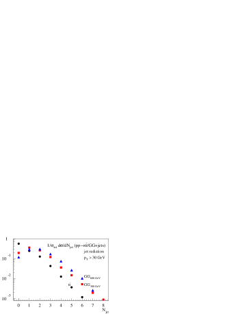
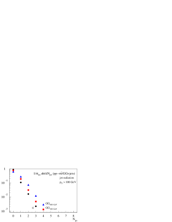
Figure 3: Number of additional jets with a transverse momentum of at least 30 or 100 GeV radiated from top pair production and the production of heavy states at the LHC. As an example for such heavy states we use a pair of scalar gluons with a mass of 300 or 600 GeV, pair-produced in gluon fusion. The figures are from a forthcoming paper with Tim Tait (arXiv:0810:3919), produced with MadEvent using it’s modified MLM algorithm — thanks to Johan Alwall.

	MC@NLO (Herwig)	CKKW (Sherpa)
hard jets	first jet correct	all jets correct
collinear jets	all jets correct, tuned	all jets correct, tuned
normalization	correct to NLO	correct to LO plus real emission
variants	Powheg,…	MLM–Alpgen, MadEvent,…

Table 2: Comparison of the MC@NLO and CKKW schemes combining collinear and hard jets.

To summarize, we can use the CKKW or MLM schemes to combine $n$-jet events with variable $n$ and at the same time combine matrix element and parton shower descriptions of the jet kinematics. In other words, we can for example simulate $Z+n$ jets production at the LHC, where all we have to do is cut off the number of jets at some point where we cannot compute the matrix element anymore. This combination will describe all jets correctly over the entire collinear and hard phase space. In Fig.3 we show the number of jets produced in association with a pair of top quarks and a pair of heavy new states at the LHC. The details of these heavy scalar gluons are secondary for the basic features of these distributions, the only parameter which matters is their mass, i.e.  the hard scale of the process which sets the factorization scale and defines the upper limit of collinearly enhanced initial-state radiation. We see that heavy states tend to come with several jets radiated with transverse momenta up to 30 GeV, where most of these jets vanish once we require transverse momenta of at least 100 GeV. Looking at this figure you can immediately see that a suggested analysis which for example asks for a reconstruction of two $W$ decay jets better give you a very good argument why it should not we swamped by combinatorics.

Looking at the individual columns in Fig.3 there is one thing we have to keep in mind: each of the merged matrix elements combined into this sample is computed at leading order, the emission of real particles is included, while virtual corrections are not (completely) there. In other words, in contrast to MC@NLO this procedure gives us all jet distributions but leaves the normalization free, just like an old-fashioned Monte Carlo. The main features and shortcomings of the two merging schemes are summarized in Tab.2. A careful study of the associated theory errors for example for $Z$+jets production and the associated rates and shapes I have not yet come across, but watch out for it.

As mentioned before — there is no such thing as a free lunch, and it is up to the competent user to pick the scheme which suits their problem best. If there is a well-defined hard scale in the process, the old-fashioned Monte Carlo with a tuned parton shower will be fine, and it is by far the fastest method. Sometimes we are only interested in one hard jet, so we can use MC@NLO and benefit from the correct normalization. And in other cases we really need a large number of jets correctly described, which means CKKW and some external normalization. This decision is not based on chemistry, philosophy or sports, it is based on QCD. What we LHC phenomenologists have to do is to get it right and know why we got it right.

On the other hand I am not getting tired of emphasizing that the conceptual progress in QCD describing jet radiation for all transverse-momentum scales is absolutely crucial for LHC analyses. If I were a string theorist I would definitely call this achievement a revolution or even two, like 1917 but with the trombones and cannons of Tchaikovsky’s 1812. In contrast to a lot of progress in theoretical physics jet merging solves a very serious problem which would have limited our ability to understand LHC data, no matter what kind of Higgs or new physics we are looking for. And I am not sure if I got the message across — the QCD aspects behind it are not trivial at all. If you feel like looking at a tough problem, try to prove that CKKW and MLM work for initial-state and final-state radiation…

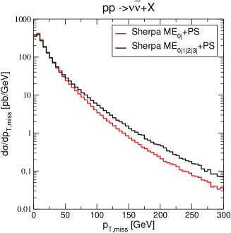
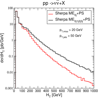
Figure 4: Transverse momentum and $H_{T}$ distributions for $Z$+jets production at the LHC. The two curves correspond to the Sherpa parton shower starting from Drell–Yan production and the fully merged sample including up to three hard jets. These distributions describe typical backgrounds for searches for jets plus missing energy, which could originate in supersymmetric squark and gluino production. Thank you to Steffen Schumann and Sherpa for providing these Figures.

Before we move on, let me illustrate why in Higgs or exotics searches at the LHC we really care about this kind of progress in QCD. One way to look for heavy particles decaying into jets, leptons and missing energy is the variable

$$H_{T} =/\!\!\!\!E_{T}+\sum_{j}E_{T,j}+\sum_{\ell}E_{T,\ell}$$

$$=/\!\!\!\!p_{T}+\sum_{j}p_{T,j}+\sum_{\ell}p_{T,\ell}\qquad\text{(for massless quarks, leptons)}$$ (47)

which for gluon-induced QCD processes should be as small as possible, while the signal’s scale will be determined by the new particle masses. For the background process $Z$+jets, this distribution as well as the missing energy distribution using CKKW as well as a parton shower (both from Sherpa) are shown in Fig. 4. The two curves beautifully show that the naive parton shower is not a good description of QCD background processes to the production of heavy particles. We can probably use a chemistry approach and tune the parton shower to correctly describe the data even in this parameter region, but we would most likely violate basic concepts like factorization. How much you care about this violation is up to you, because we know that there is a steep gradient in theory standards from first-principle calculations of hard scattering all the way to hadronization string models…

V Simulating LHC events

In the third main section I will try to cover a few topics of interest to LHC physicists, but which are not really theory problems. Because they are crucial for our simulations of LHC signatures and can turn into sources of great embarrassment when we get them wrong in public.

V.1 Missing energy

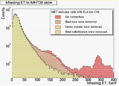
Figure 5: Missing energy distribution from the early running phase of the DZero experiment at the Tevatron. This figure I got from Beate Heinemann’s lectures web site.

Some of the most interesting signatures at the LHC involve dark matter particles. Typically, we would produce strongly interacting new particles which then decay to the weakly interacting dark matter agent. On the way, the originally produced particles have to radiate quarks or gluons, to get rid of their color charge. If they also radiate leptons, those can be very useful to trigger on the events and reduce QCD backgrounds.

At the end of the last section we talked about the proper simulation of $W$+jets and $Z$+jets backgrounds to such signals. It turns out that jet merging predicts considerably larger missing transverse momentum from QCD sources, so theoretically we are on fairly safe ground. However, this is not the whole story of missing transverse momentum. I should say that I skipped most of this section, because Peter Wittich knows much more about it and covered it really nicely. But it might nevertheless be useful to include it in this writeup.

Fig. 5 is a historic missing transverse energy distribution from DZero. It nicely illustrates that by just measuring missing energy, Tevatron would have discovered supersymmetry with two beautiful peaks in the missing-momentum distribution around 150 GeV and around 350 GeV. However, this distribution has nothing to do with physics, it is purely a detector effect.

The problem of missing energy can be illustrated with a simple number: to identify and measure a lepton we need around 500 out of 200000 calorimeter cells in an experiment like Atlas, while for missing energy we need all of them. Therefore, we need to understand our detectors really well to even cut on a variable like missing transverse momentum, and for this level of understanding we need time and luminosity. Unless something goes wrong with the machine, I would not expect us to find anything reasonable in early-running LHC data including a missing energy cut — really, we should not use the phrases ‘missing energy’ and ‘early running’ in the same sentences or papers.

There are three sources of missing energy which our experimental colleagues have to understand before we get to look at such distributions:

First, we have to subtract bad runs. This means that for a few hours parts of the detector might not have worked properly. We can identify such bad runs by looking at Standard Model physics, like gauge bosons, and remove them from the data sample.

Next, there is usually coherent noise in the calorimeter. Of 200000 cells we know that some of them will individually fail or produce noise. However, some sources of noise, like leaking voltage or other electronic noise can be correlated geometrically, i.e.  coherent. Such noise will lead to beautiful missing momentum signals. In the same spirit, there might also be particles crossing our detector, but not coming from the interaction point. Such particles can be cosmic rays or errand beam radiation, and they will lead to unbalanced energy deposition in the calorimeter. The way to get rid of such noise is again looking for Standard Model candles and remove sets of events where such problems occur.

The third class of fake missing energy is failing calorimeter cells, like continuously hot cells or dead cells, which can be removed after we know the detector really well.

Once we understand all the source of fake missing momentum we can focus on real missing momentum. This missing transverse momentum is trivially computed from the momentum measurement of all tracks seen in the detector. This means that any uncertainty on these measurements, like the jet or lepton energy scale will smear the missing momentum. Moreover, we know that there is for example dead matter in the detector, so we have to compensate for this. This compensation is obviously a global correction to individual events, which means it will generally smear the missing energy distribution. So when we compute a realistic missing transverse momentum distribution at the LHC we have to smear all jet and lepton momenta, and in addition apply a Gaussian smearing of the order

$$\frac{\Delta/\!\!\!\!E_{T}}{\text{GeV}}\sim\frac{1}{2}\;\sqrt{\frac{\sum E_{T}}{\text{GeV}}}\;\gtrsim 20$$ (48)

While this sounds like a trivial piece of information I cannot count the number of papers I get to referee where people forgot this smearing and discovered great channels to look for Higgs bosons or new physics at the LHC which completely fall apart when experimentalists take a careful look. Here comes another great piece of phenomenology wisdom: phenomenological studies are right or wrong based on the outcome if they can be reproduced by real experimentalists and real detectors — at least once we make sure our experimentalist friends did not screw it up again….

V.2 Phase space integration

At the very beginning of this lecture we discussed how to compute the total cross section for interesting processes. What we skipped is how to numerically compute such cross sections. Obviously, since the parton densities are not known in a closed analytical form, we will have to rely on numerical integration tools. Looking at a simple $2\to 2$ process we can write the total cross section as

$$\sigma_{\rm tot}=\int d\phi\int d\cos\theta\int dx_{1}\int dx_{2}\;F_{\rm PS}\left|\mathcal{M}\right|^{2}=\int_{0}^{1}dy_{1}\cdots dy_{4}\;J_{\rm PS}(\vec{y})\left|\mathcal{M}\right|^{2}$$ (49)

The different factors are shown in eq.(21). In the second step we have rewritten the phase space integral as an integral over the four–dimensional unit cube, with the appropriate Jacobian. Like any integral we can numerically evaluate this phase space integral by binning the variable we integrate over:

$$\int_{0}^{1}dy\;f(y)\quad\longrightarrow\quad\sum_{j}(\Delta y)_{j}f(y_{j})\sim\Delta y\sum_{j}f(y_{j})$$ (50)

Whenever we talk about numerical integration we can without any loss of generality assume that the integration boundaries are 0…1. The integration variable $y$ we can divide into a discrete set of points $y_{j}$, for example defined as equi-distant on the $y$ axis or by choosing some kind of random number $y_{j}\epsilon[0,1]$. In the latter case we need to keep track of the bin widths $(\Delta y)_{j}$. In a minute, we will discuss how such a random number can be chosen in more or less smart ways; but before we discuss how to best evaluate such an integral numerically, let us first illustrate that this integral is much more useful than just providing the total cross section. If we are interested in a distribution of an observable, like for example the distribution of the transverse momentum of a muon in the Drell–Yan process, we need to compute $d\sigma(p_{T})/dp_{T}$. This distribution is given by:

$$\sigma =\int dy_{1}\cdots dy_{N}\;f(\vec{y})=\int dy_{1}\;\frac{d\sigma}{dy_{1}}$$

$$\frac{d\sigma}{dy_{1}}\Bigg{|}_{y_{1}^{0}} =\int dy_{2}\cdots dy_{N}\;f(y_{1}^{0})=\int dy_{1}\cdots dy_{N}\;f(\vec{y})\;\delta(y_{1}-y_{1}^{0})$$ (51)

We can compute this distribution numerically in two ways. One way would be to numerically evaluate the $y_{2}\cdots y_{N}$ integrations and just leave out the $y_{1}$ integration. The result will be a function of $y_{1}$ which we can evaluate at any point $y_{1}^{0}$. This method is what I for example used for Prospino, when I was a graduate student. The second and much smarter option corresponds to the last term in the equation above, with the delta distribution defined for discretized $y_{1}$. This is not hard to do: first, we define an array the size of the number of bins in the $y_{1}$ integration. Then, for each $y_{1}$ value of the complete $y_{1}\cdots y_{N}$ integration we decide where it goes in this array and add $f(\vec{y})$ to this array. And finally, we print $f(y_{1})$ to see the distribution. This array is referred to as a histogram and can be produced for example using the CernLib. This histogram approach does not look like much, but imagine you want to compute a distribution $d\sigma/dp_{T}$, where $p_{T}(\vec{y})$ is a complicated function of the integration variables, so you want to compute:

$$\frac{d\sigma}{dp_{T}}=\int dy_{1}\cdots dy_{N}\;f(\vec{y})\;\delta\left(p_{T}(\vec{y})-p_{T}^{0}\right)$$ (52)

Histograms mean that when we compute the total cross section entirely numerically we can trivially extract all distributions in the same process.

The procedure outlined above has an interesting interpretation. Imagine we do the entire phase space integrations numerically. Just like computing the interesting observables we can compute the momenta of all external particles. These momenta are not all independent, because of energy–momentum conservation, but this can be taken care of. The tool which translates the vector of integration variables $\vec{y}$ into the external momenta is called a phase space generator. Because the phase space is not uniquely defined in terms of the integration variables, the phase space generator also has to return the Jacobian $J_{\rm PS}$, the phase space weight. If we think of the integration as an integration over the unit cube, this weight is combined with the matrix element squared $\left|\mathcal{M}\right|^{2}$. Once we compute the unique phase space configuration $(k_{1},k_{2},p_{1}\cdots p_{M})_{j}$ which corresponds to the vector $\vec{y}_{j}$ the combined weight $W=J_{\rm PS}\left|\mathcal{M}\right|^{2}$ is simply the probability that this configuration will appear at the LHC. Which means, we do not only integrate over the phase space, we really simulate events at the LHC. The only complication is that the probability of a certain configuration is not only given my the frequency with which it appears, but also by the additional explicit weight. So when we run our numerical integration through the phase space generator and histogram all the distributions we are interested in we really generate weighted events. These events, i.e.  the momenta of all external particles and the weight $W$, we can for example store in a big file.

This simulation is not quite what experimentalists want — they want to represent the probability of a certain configuration appearing only by its frequency. This means we have to unweight the events and translate the weight into frequency. To achieve this we normalize all our event weights to the maximum weight $W_{\rm max}$, i.e.  compute the ratio $W_{j}/W_{\rm max}\epsilon[0,1]$, generate a flatly distributed random number $r\epsilon[0,1]$, and keep the event if $W_{j}/W_{\rm max}>r$. This guarantees that each event $j$ survives with a probability $W_{j}/W_{\rm max}$, which is exactly what we want — the higher the weight the more likely the event stays. The challenge in this translation is only that we will lose events, which means that our distributions will if anything become more ragged. So if it weren’t for the experimentalists we would never use unweighted events. I should add that experimentalists have a good reason to want such unweighted events, because they feed best through their detector simulations.

The last comment is that if the phase space configuration $(k_{1},k_{2},p_{1}\cdots p_{M})_{j}$ can be measured, its weight $W_{j}$ better be positive. This is not trivial once we go beyond leading order. There, we need to add several contributions to produce a physical event, like for example different $n$–particle final states, and there is no need for all of them to be positive. All we have to guarantee is that after adding up all contributions and after integrating over any kind of unphysical degree of freedom we might have introduced, the probability of a physics configuration is positive. For example, negative values for parton densities are not problematic, as long as we always have a positive hadronic rate $d\sigma_{pp\to X}>0$.

The numerical phase space integration for many particles faces two problems. First, the partonic phase space for $M$ on-shell particles in the final state has $3(M+2)-3$ dimensions. If we divide each of these directions in 100 bins, the number of phase space points we need to evaluate for a $2\to 4$ process is $100^{15}=10^{30}$, which is not realistic.

To integrate over a large number of dimensions we use Monte Carlo integration. In this approach we define a distribution $p_{Y}(y)$ such that for a one-dimensional integral we can replace the binned discretized integral in eq.(50) with a discretized version based on a set of random numbers $Y_{j}$ over the $y$ integration space

$$\langle g(Y)\rangle=\int_{0}^{1}dy\;p_{Y}(y)\;g(y)\quad\longrightarrow\quad\frac{1}{N}\sum_{j}g(Y_{j})$$ (53)

All we have to make sure is that the probability of returning $Y_{j}$ is given by $p_{Y}(y)$ for $y<Y_{j}<y+dy$. This form has the advantage that we can naively generalize it to any number of $n$ dimensions, just by organizing the random numbers $Y_{j}$ in one large vector instead of an $n$-dimensional array.

Our $n$-dimensional phase space integral listed above we can rewrite the same way:

$$\int_{0}^{1}d^{n}y\;f(y)=\int_{0}^{1}d^{n}y\;\frac{f(y)}{p_{Y}(y)}\;p_{Y}(y)=\left<\frac{f(Y)}{p_{Y}(Y)}\right>\quad\longrightarrow\quad\frac{1}{N}\sum_{j}\frac{f(Y_{j})}{p_{Y}(Y_{j})}$$ (54)

In other words, we have written the phase space integral in a discretized way which naively does not involve the number of dimensions any longer. All we have to do to compute the integral is average over $N$ phase space values of $f/p_{Y}$. In the ideal case where we exactly know the form of the integrand and can map it into our random numbers, the error of the numerical integration will be zero. So what we have to find is a way to encode $f(Y_{j})$ into $p_{Y}(Y_{j})$. This task is called importance sampling and you will have to find some documentation for example on Vegas to look at the details.

Technically, you will find that Vegas will call the function which computes the weight $W=J_{\rm PS}|\mathcal{M}|^{2}$ for a number of phase space points and average over these points, but including another weight factor $W_{\rm MC}$ representing the importance sampling. If you want to extract distributions via histograms you have to therefore add the total weight $W=W_{\rm MC}J_{\rm PS}|\mathcal{M}|^{2}$ to the columns.

The second numerical challenge is that the matrix elements for interesting processes are by no means flat, and we would like to help our adaptive (importance sampling) Monte Carlo by defining the integration variables such that the integrand is as flat as possible. Take for example the integration over the partonic momentum fraction, where the integrand is usually falling off at least as $1/x$. So we can substitute

$$\int_{\delta}dx\;\frac{C}{x}=\int_{\log\delta}d\log x\;\left(\frac{d\log x}{dx}\right)^{-1}\;\frac{C}{x}=\int_{\log\delta}d\log x\;C$$ (55)

and improve our integration significantly. Moving on to a more relevant example: particularly painful are intermediate particles with Breit–Wigner propagators squared, which we need to integrate over the momentum $s=p^{2}$ flowing through:

$$P(s,m)=\frac{1}{(s-m^{2})^{2}+m^{2}\Gamma^{2}}$$ (56)

For example the Standard-Model Higgs boson with a mass of 120 GeV has a width around $0.005$ GeV, which means that the integration over the invariant mass of the Higgs decay products $\sqrt{s}$ requires a relative resolution of $10^{-5}$. Since this is unlikely to be achievable, what we should really do is find a substitution which produces the inverse Breit–Wigner as a Jacobian and leads to a flat integrand — et voilá

$$\int ds\;\frac{C}{(s-m^{2})^{2}+m^{2}\Gamma^{2}} =\int dz\;\left(\frac{dz}{ds}\right)^{-1}\frac{C}{(s-m^{2})^{2}+m^{2}\Gamma^{2}}$$

$$=\int dz\;\frac{(s-m^{2})^{2}+m^{2}\Gamma^{2}}{m\Gamma}\;\frac{C}{(s-m^{2})^{2}+m^{2}\Gamma^{2}}$$

$$=\frac{1}{m\Gamma}\int dz\;C\qquad\text{with}\qquad\tan z=\frac{s-m^{2}}{m\Gamma}$$ (57)

This is the coolest phase space mapping I have seen, and it is incredibly useful. Of course, an adaptive Monte Carlo will eventually converge on such an integrand, but a well-chosen set of integration parameters will speed up our simulations significantly.

V.3 Helicity amplitudes

When we compute a transition amplitude, what we usually do is write down all spinors, polarization vectors, interaction vertices and propagators and square the amplitude analytically to get $|\mathcal{M}|^{2}$. Of course, nobody does gamma–matrix traces by hand anymore, instead we use powerful tools like Form. But we can do even better. As an example, let us consider the simple process $u\bar{u}\to\gamma^{*}\to\mu^{+}\mu^{-}$. The structure of the amplitude in the Dirac indices involves one vector current on each side $(\bar{u}_{f}\gamma_{\mu}u_{f})$. For each $\mu=0\cdots 3$ this object gives a c-number, even though the spinors have four components and each gamma matrix is a $4\times 4$ matrix as well. The intermediate photon propagator has the form $g_{\mu\nu}/s$, which is a simple number as well and implies a sum over $\mu$ in both of the currents forming the matrix element.

Instead of squaring this amplitude symbolically we can first compute it numerically, just inserting the correct numerical values for each component of each spinor etc, without squaring it. MadGraph is a tool which automatically produces a Fortran routine which calls the appropriate functions from the Helas library, to do precisely that. For our toy process the MadGraph output looks roughly like:

      REAL*8 FUNCTION UUB_MUPMUM(P,NHEL)
C
C FUNCTION GENERATED BY MADGRAPH
C RETURNS AMPLITUDE SQUARED SUMMED/AVG OVER COLORS
C FOR PROCESS : u u~ -> mu+ mu-
C
      INTEGER    NGRAPHS,    NEIGEN,    NEXTERNAL
      PARAMETER (NGRAPHS=   1,NEIGEN=  1,NEXTERNAL=4)
      INTEGER    NWAVEFUNCS     , NCOLOR
      PARAMETER (NWAVEFUNCS=   5, NCOLOR=   1)

      REAL*8 P(0:3,NEXTERNAL)
      INTEGER NHEL(NEXTERNAL)

      INCLUDE ’coupl.inc’

      DATA Denom(1  )/            1/
      DATA (CF(i,1  ),i=1  ,1  ) /     3/

      CALL IXXXXX(P(0,1   ),ZERO ,NHEL(1   ),+1,W(1,1   ))
      CALL OXXXXX(P(0,2   ),ZERO ,NHEL(2   ),-1,W(1,2   ))
      CALL IXXXXX(P(0,3   ),ZERO ,NHEL(3   ),-1,W(1,3   ))
      CALL OXXXXX(P(0,4   ),ZERO ,NHEL(4   ),+1,W(1,4   ))
      CALL JIOXXX(W(1,1   ),W(1,2   ),GAU ,ZERO    ,ZERO    ,W(1,5   ))
      CALL IOVXXX(W(1,3   ),W(1,4   ),W(1,5   ),GAL ,AMP(1   ))
      JAMP(   1) = +AMP(   1)

      DO I = 1, NCOLOR
          DO J = 1, NCOLOR
              ZTEMP = ZTEMP + CF(J,I)*JAMP(J)
          ENDDO
          UUB_MUPMUM =UUB_MUPMUM+ZTEMP*DCONJG(JAMP(I))/DENOM(I)
      ENDDO
      END

The input to this function are the external momenta and the helicities of all fermions in the process. Remember that helicity and chirality are identical only for massless fermions. In general, chirality is defined as the eigenvalue of the projectors $(\leavevmode\hbox{\small 1\normalsize\kern-3.30002pt1}\pm\gamma_{5})/2$, while helicity is defined as the projection of the spin onto the momentum direction, or as the left or right handedness. For each point in phase space and each helicity combination ($\pm 1$ for each external fermion) MadGraph computes the matrix element using Helas routines like for example:

• IXXXXX($p,m,n_{\rm hel},n_{\rm sf},F$) computes the wave function of a fermion with incoming fermion number, so either an incoming fermion or an outgoing anti-fermion. As input it requires the 4-momentum, the mass and the helicity of this fermion. Moreover, this particle with incoming fermion number can be a particle or an anti-particle. This means $n_{\rm fs}=+1$ for the incoming $u$ and $n_{\rm sf}=-1$ for the outgoing $\mu^{+}$, because the particles in MadGraph are defined as $u$ and $\mu^{-}$. The fermion wave function output is a complex array $F(1:6)$.

  Its first two entries are the left-chiral part of the fermionic spinor, i.e.  $F(1:2)=(\leavevmode\hbox{\small 1\normalsize\kern-3.30002pt1}-\gamma_{5})/2\;u$ or $F(1:2)=(\leavevmode\hbox{\small 1\normalsize\kern-3.30002pt1}-\gamma_{5})/2\;v$ for $n_{\rm sf}=\pm 1$. The entries $F(3:4)$ are the right-chiral spinor. These four numbers can be computed from the 4-momentum, if we know the helicity of the particles. Because for massless particles helicity and chirality are identical, our massless quarks and leptons will for example have only entries $F(1:2)$ for $n_{\rm hel}=-1$ and $F(3:4)$ for $n_{\rm hel}=+1$.

  The last two entries contain the 4-momentum in the direction of the fermion flow, namely $F(5)=n_{\rm sf}(p(0)+ip(3))$ and $F(6)=n_{\rm sf}(p(1)+ip(2))$. The first four entries in this spinor correspond to the size of each $\gamma$ matrix, which is usually taken into account by computing the trace of the chain of gamma matrices.

• OXXXXX($p,m,n_{\rm hel},n_{\rm sf},F$) does the same for a fermion with outgoing fermion flow, i.e.  our incoming $\bar{u}$ and our outgoing $\mu^{-}$. The left-chiral and right-chiral components now read $F(1:2)=\bar{u}(\leavevmode\hbox{\small 1\normalsize\kern-3.30002pt1}-\gamma_{5})/2$ and $F(3:4)=\bar{u}(\leavevmode\hbox{\small 1\normalsize\kern-3.30002pt1}+\gamma_{5})/2$, and similarly for the spinor $\bar{v}$. The last two entries are $F(5)=n_{\rm sf}(p(0)+ip(3))$ and $F(6)=n_{\rm sf}(p(1)+ip(2))$.

• JIOXXX($F_{i},F_{o},g,m,\Gamma,J_{io}$) computes the (off-shell) current for the vector boson attached to the two external fermions $F_{i}$ and $F_{o}$. The coupling $g(1:2)$ is a complex array with the interaction of the left-chiral and right-chiral fermion in the upper and lower index. Obviously, we need to know the mass and the width of the intermediate vector boson. The output array $J_{io}$ again has six components:

  $$J_{io}(\mu+1) =-\frac{i}{q^{2}}\;F_{o}^{T}\;\gamma^{\mu}\left(g(1)\;\frac{\leavevmode\hbox{\small 1\normalsize\kern-3.30002pt1}-\gamma_{5}}{2}\;+g(2)\;\frac{\leavevmode\hbox{\small 1\normalsize\kern-3.30002pt1}+\gamma_{5}}{2}\;\right)\;F_{i}$$

  $$J_{io}(5) =-F_{i}(5)+F_{o}(5)\sim-p_{i}(0)+p_{o}(0)+i\left(-p_{i}(3)-p_{o}(3)\right)$$

  $$J_{io}(6) =-F_{i}(6)+F_{o}(6)\sim-p_{i}(1)+p_{o}(1)+i\left(-p_{i}(2)+p_{o}(2)\right)$$

  $$\Rightarrow\qquad q^{\mu} =\left(\text{Re}J_{io}(5),\text{Re}J_{io}(6),\text{Im}J_{io}(6),\text{Im}J_{io}(5)\right)$$ (58)

  The last line illustrates why we need the fifth and sixth arguments of $F_{io}$. The first four entries in $J_{io}$ correspond to the index $\mu$ in this vector current, while the index $j$ of the spinors has been contracted between $F_{o}^{T}$ and $F_{i}$.

• IOVXXX($F_{i},F_{o},J,g,V$) computes the amplitude of a fermion–fermion–vector coupling using the two external fermionic spinors $F_{i}$ and $F_{o}$ and an incoming vector current $J$. Again, the coupling $g(1:2)$ is a complex array, so we numerically compute

  $$F_{o}^{T}\;/\!\!\!\!J\left(g(1)\;\frac{\leavevmode\hbox{\small 1\normalsize\kern-3.30002pt1}-\gamma_{5}}{2}\;+g(2)\;\frac{\leavevmode\hbox{\small 1\normalsize\kern-3.30002pt1}+\gamma_{5}}{2}\;\right)\;F_{i}$$ (59)

  We see that all indices $j$ and $\mu$ of the three input arguments are contracted in the final result. Momentum conservation is not explicitly enforced by IOVXXX, so we have to take care of it beforehand.

Given the list above it is easy to see how MadGraph computes the amplitude for $u\bar{u}\to\gamma^{*}\to\mu^{+}\mu^{-}$. First, it always calls the wave functions for all external particles and puts them into the array $W(1:6,1:4)$. The vectors $W(*,1)$ and $W(*,3)$ correspond to $F_{i}(u)$ and $F_{i}(\mu^{+})$, while $W(*,2)$ and $W(*,4)$ mean $F_{o}(\bar{u})$ and $F_{o}(\mu^{-})$. The first vertex we evaluate is the $\bar{u}\gamma u$ vertex, which given $F_{i}=W(*,1)$ and $F_{o}=W(*,2)$ uses JIOXXX to compute the vector current for the massless photon in the $s$ channel. Not much would change if we instead chose a massive $Z$ boson, except for the arguments $m$ and $\Gamma$ in the JIOXXX call. The JIOXXX output is the photon current $J_{io}\equiv W(*,5)$. The second step combines this current with the two outgoing muons in the $\mu^{+}\gamma\mu^{-}$ vertex. Since this number gives the final amplitude, it should return a c-number, no array. MadGraph calls IOVXXX with $F_{i}=W(*,3)$ and $F_{o}=W(*,4)$, combined with the photon current $J=W(*,5)$. The result AMP is copied into JAMP without an additional sign which could have come from the ordering of external fermions. The only remaining sum left to compute before we square JAMP is the color structure, which in our simple case means one color structure with a color factor $N_{c}=3$.

Of course, to calculate the transition amplitude MadGraph requires all masses and couplings. They are transferred through common blocks in the file coupl.inc and computed elsewhere. In general, MadGraph uses unitary gauge for massive vector bosons, because in the helicity amplitude approach it is easy to accommodate complicated tensors, in exchange for a large number of Feynman diagrams.

The function UUB_MUPMUM described above is not yet the full story. Remember that when we square $\mathcal{M}$ symbolically we need to sum over the spins of the outgoing states to transform a spinor product of the kind $u\bar{u}$ into the residue or numerator of a fermion propagator. To obtain the final result numerically we also need to sum over all possible helicity combinations of the external fermions, in our case $2^{4}=16$ combinations.

      SUBROUTINE SUUB_MUPMUM(P1,ANS)
C
C FUNCTION GENERATED BY MADGRAPH
C RETURNS AMPLITUDE SQUARED SUMMED/AVG OVER COLORS
C AND HELICITIES FOR THE POINT IN PHASE SPACE P(0:3,NEXTERNAL)
C
C FOR PROCESS : u u~ -> mu+ mu-
C
      INTEGER    NEXTERNAL,   NCOMB,
      PARAMETER (NEXTERNAL=4, NCOMB= 16)
      INTEGER    THEL
      PARAMETER (THEL=NCOMB*1)

      REAL*8 P1(0:3,NEXTERNAL),ANS

      INTEGER NHEL(NEXTERNAL,NCOMB),NTRY
      REAL*8 T, UUB_MUPMUM
      INTEGER IHEL,IDEN,IC(NEXTERNAL)
      INTEGER IPROC,JC(NEXTERNAL)
      LOGICAL GOODHEL(NCOMB)

      DATA GOODHEL/THEL*.FALSE./
      DATA NTRY/0/

      DATA (NHEL(IHEL,  1),IHEL=1,4) / -1, -1, -1, -1/
      DATA (NHEL(IHEL,  2),IHEL=1,4) / -1, -1, -1,  1/
      DATA (NHEL(IHEL,  3),IHEL=1,4) / -1, -1,  1, -1/
      DATA (NHEL(IHEL,  4),IHEL=1,4) / -1, -1,  1,  1/
      DATA (NHEL(IHEL,  5),IHEL=1,4) / -1,  1, -1, -1/
      DATA (NHEL(IHEL,  6),IHEL=1,4) / -1,  1, -1,  1/
      DATA (NHEL(IHEL,  7),IHEL=1,4) / -1,  1,  1, -1/
      DATA (NHEL(IHEL,  8),IHEL=1,4) / -1,  1,  1,  1/
      DATA (NHEL(IHEL,  9),IHEL=1,4) /  1, -1, -1, -1/
      DATA (NHEL(IHEL, 10),IHEL=1,4) /  1, -1, -1,  1/
      DATA (NHEL(IHEL, 11),IHEL=1,4) /  1, -1,  1, -1/
      DATA (NHEL(IHEL, 12),IHEL=1,4) /  1, -1,  1,  1/
      DATA (NHEL(IHEL, 13),IHEL=1,4) /  1,  1, -1, -1/
      DATA (NHEL(IHEL, 14),IHEL=1,4) /  1,  1, -1,  1/
      DATA (NHEL(IHEL, 15),IHEL=1,4) /  1,  1,  1, -1/
      DATA (NHEL(IHEL, 16),IHEL=1,4) /  1,  1,  1,  1/
      DATA (  IC(IHEL,  1),IHEL=1,4) /  1,  2,  3,  4/
      DATA (IDEN(IHEL),IHEL=  1,  1) /  36/

      NTRY=NTRY+1

      DO IHEL=1,NEXTERNAL
         JC(IHEL) = +1
      ENDDO

      DO IHEL=1,NCOMB
         IF (GOODHEL(IHEL,IPROC) .OR. NTRY .LT. 2) THEN
            T = UUB_MUPMUM(P1,NHEL(1,IHEL),JC(1))
            ANS = ANS + T
            IF (T .GT. 0D0 .AND. .NOT. GOODHEL(IHEL,IPROC)) THEN
               GOODHEL(IHEL,IPROC)=.TRUE.
            ENDIF
         ENDIF
      ENDDO
      ANS = ANS/DBLE(IDEN)

      END

The important part of this subroutine is the list of possible helicity combinations stored in the array NHEL$(1:4,1:16)$. Adding all different helicity combinations (of which some might well be zero) means a loop over the second argument and a call of UUB_MUPMUM with the respective helicity combination. The complete spin–color averaging factor is included as IDEN and given by $2\times 2\times N_{c}^{2}=36$. So MadGraph indeed provides us with a subroutine SUUB_MUPMUM which numerically computes $\overline{|\mathcal{M}|^{2}}$ for each phase space point, i.e.  external momentum configuration. MadGraph also produces a file with all Feynman diagrams contributing to the given subprocess, in which the numbering of the external particles corresponds to the second argument of $W$ and the argument of AMP is the numbering of the Feynman diagrams. After looking into the code very briefly we can also easily identify different intermediate results $W$ which will only be computed once, even if they appear several times in the different Feynman diagrams.

The helicity method might not seem particularly appealing for a simple $2\to 2$ process, but it makes it easily possible to compute processes with four and more particles in the final state and up to 10000 Feynman diagrams which we could never square symbolically, no matter how many graduate students’ lives we turn into hell.

V.4 Errors

As argued in the very beginning of the lecture, LHC physics always means extracting signals from often large backgrounds. This means, a correct error estimate is crucial. For LHC calculations we are usually confronted with three types of errors.

The first and easiest one are the statistical errors. For small numbers of events these experimental errors are described by Poisson statistics, and for large numbers they converge to the Gaussian limit. And that is about the only complication we encounter for them.

The second set of errors are systematic errors, like for example the calibration of the jet and lepton energy scales, the measurements of the luminosity, or the efficiencies to identify a muon as a muon. Some of you might remember what happened last, when a bunch of theorists mistook a forward pion for an electron — that happened right around my TASI, and people had not only discovered supersymmetry, but also identified its breaking mechanism. Of course, our experimentalist CDF lecturer told us immediately that the whole thing was a joke. Naively, we would not assume that systematic are Gaussian, but remember that we determine these numbers largely from well-understood background processes. Such counting experiments in background channels like $Z\to$ leptons, however, do behave Gaussian. The only caveat is the shape of far-away tails, which can turn out to be bigger than the exponentially suppressed Gaussian shape.

The last source of errors are theory errors, and they are hardest to model, because they are dominated by higher-order QCD effects, fixed order or enhanced by large logarithms. If we could compute all remaining higher-order terms, we would do so, which means everything else is a wild guess. Moreover, higher-order effects are not any more likely to give a relative $K$ factor of 1.0 than 0.9 or 1.1. In other words, theory errors cannot have a peak and they are definitely not Gaussian. There is a good reason to choose the Gaussian short cut, because we know that folding three Gaussian errors gives us another Gaussian error, which makes things so much easier. But this lazy approach assumes the we know much more about QCD than we actually do, so please stop lying. On the other hand, we also know that theory errors cannot be arbitrarily large. Unless there is a very good reason, a $K$ factor for a total LHC cross section should not be larger than something like 3. If that were the case, we would conclude that perturbative QCD breaks down, and the proper description of error bars would be our smallest problem. In other words, the centrally flat theory probability distribution for an LHC observable has to go to zero for very large deviations from the currently best value.

A good solution to this problem is the so-called Rfit scheme, used for example by the CKMfitter or the SFitter collaborations. It starts from the assumption that for very large deviations there will always be tails from the experimental errors, so we can neglect the impact of the theory errors on this range. In the center of the distribution we simply cut open the experimental Gaussian-type distribution and insert a flat theory piece. We could also modify the transition region by changing for example the width of the experimental Gaussian error as an effect of a falling-off theory error, but in the simplest model we just use a log-likelihood $\chi^{2}=-2\log\mathcal{L}$ given a set of measurements $\vec{d}$ and in the presence of a general correlation matrix $C$

$$\chi^{2} ={\vec{\chi}_{d}}^{T}\;C^{-1}\;\vec{\chi}_{d}$$

$$\chi_{d,i} =\begin{cases}0&|d_{i}-\bar{d}_{i}|<\sigma^{\text{(theo)}}_{i}\\ \frac{\displaystyle d_{i}-\bar{d}_{i}+\sigma^{\text{(theo)}}_{i}}{\displaystyle\sigma^{\text{(exp)}}_{i}}&\;d_{i}-\bar{d}_{i}\;<-\sigma^{\text{(theo)}}_{i}\\ \frac{\displaystyle d_{i}-\bar{d}_{i}-\sigma^{\text{(theo)}}_{i}}{\displaystyle\sigma^{\text{(exp)}}_{i}}\qquad&\;d_{i}-\bar{d}_{i}\;>\sigma^{\text{(theo)}}_{i}\;.\end{cases}$$ (60)

And that is it, all three sources of LHC errors can be described correctly, and nothing stops us from computing likelihood maps to measure the top mass or identify new physics or just have some fun in life at the expense of the Grid.

Further reading, acknowledgments, etc.

This is the point where the week in beautiful Boulder is over and I should thank K.T. and his Boulder team as well as our two organizers for their kind invitation. I typed most of these notes in Boulder’s many nice cafes and 11 years after I went here as a student TASI and Boulder still make the most enjoyable and most productive school in our field. Whoever might ever think about moving it away from Boulder cannot possibly have the success of the school in mind.

It has been great fun, even though QCD has a reputation of being a dry topic. I hope you enjoyed learning it as much as I enjoyed learning it while teaching it. Just like most of you I am really only a QCD user, but for an LHC phenomenologists there is no excuse for not knowing the relevant aspects of QCD. Have fun in the remaining lectures, write some nice theses, and I hope I will see as many of you as possible over the coming 20 years. LHC physics need all the help we can get, and it is great fun, so please come and join us!

Of course there are many people I need to thank for helping me write these notes: Fabio Maltoni, Johan Alwall and Steffen Schumann for having endured a great number of critical questions and for convincing me that jet merging is the future; Steffen Schumann, Ben Allanach and Tom DeGrand for their comments on this draft; Beate Heinemann for providing me with one of the most interesting plots from the Tevatron and for answering many stupid questions over the years — as did Dirk Zerwas and Kyle Cranmer.

You note that this writeup, just like the lectures, is more of an informal chat about LHC physics than a proper review paper. But if I had not cut as many corners we would never have made it to the fun topics. In the same spirit, there is no point in giving you a list of proper original references, so I would rather list a few books and review articles which might come in handy if you would like to know more:

• I started learning high–energy theory including QCD from Otto Nachmann’s book. I still use his appendices to look up Feynman rules, because I have rarely seen another book with as few (if not zero) typos Nachtmann:1990ta . Similar, but maybe a little more modern is the primer by Cliff Burgess and Guy Moore Burgess:2007zi . At the end of it you will find more literature tips.

• For a more specialized book on QCD have a look at the pink book by Ellis, Stirling, Webber. It includes everything you ever wanted to know about QCD Ellis:1991qj . Maybe a little more phenomenology you can find in Günther Dissertori, Ian Knowles and Michael Schmelling’s book on QCD and phenomenology Dissertori:2003pj .

• If you would like to learn how to for example compute higher-order cross sections to Drell–Yan production, Rick Field works it all out in his book Field:1989uq .

• Unfortunately, there is comparably little literature on jet merging yet. The only review I know is by Michelangelo Mangano and Tim Stelzer Mangano:2005dj . There is a very concise discussion included with the comparison of the different models Alwall:2007fs . If you want to know more, you will have to consider the original literature or wait for the review article which Frank Krauss and Peter Richardson promised to write for Journal of Physics G.

• Recently, I ran across George Sterman’s TASI lectures. They are comparably formal, but they are a great read if you know something about QCD already Sterman:2004pd .

• For MC@NLO there is nothing like the original papers. Have a look at Bryan Webber’s and Stefano Frixione’s work and you cannot but understand what it is about Frixione:2002ik !

• For CKKW, look at the original paper. It beautifully explains the general idea on a few pages, at least for final state radiation Catani:2001cc .

• If you are using Madgraph to compute helicity amplitudes there is the original bright green documentation which describes every routine in detail. You might want to check the format of the arrays, if you use for example the updated version inside MadEvent Murayama:1992gi .

References

-
(1)
O. Nachtmann,
“Elementary Particla Physics: Concepts and Phenomena”
Berlin, Germany: Springer (1990) 559 p -
(2)
C. P. Burgess and G. D. Moore,
“The Standard Model: A Primer”
Cambridge, UK: Cambridge Univ. Pr. (2007) 542 p -
(3)
R. K. Ellis, W. J. Stirling and B. R. Webber,
“QCD and collider physics”
Camb. Monogr. Part. Phys. Nucl. Phys. Cosmol. 8, 1 (1996). -
(4)
G. Dissertori, I. G. Knowles and M. Schmelling,
“QCD — High Energy Experiments and Theory”
Oxford, UK: Clarendon (2003) 538 p -
(5)
R. D. Field,
“Applications of Perturbative QCD”
Redwood City, USA: Addison-Wesley (1989) 366 p. (Frontiers in physics, 77) -
(6)
M. L. Mangano and T. J. Stelzer,
“Tools For The Simulation Of Hard Hadronic Collisions”
Ann. Rev. Nucl. Part. Sci. 55, 555 (2005), CERN-PH-TH-2005-074. -
(7)
J. Alwall et al.,
“Comparative study of various algorithms for the merging of parton showers and matrix elements in hadronic collisions”
Eur. Phys. J. C 53, 473 (2008) [arXiv:0706.2569 [hep-ph]]. -
(8)
G. Sterman,
“QCD and jets”
arXiv:hep-ph/0412013. -
(9)
S. Frixione and B. R. Webber,
“Matching NLO QCD computations and parton shower simulations”
JHEP 0206, 029 (2002) [arXiv:hep-ph/0204244]. -
(10)
S. Catani, F. Krauss, R. Kuhn and B. R. Webber,
“QCD matrix elements + parton showers”
JHEP 0111, 063 (2001) [arXiv:hep-ph/0109231]. -
(11)
H. Murayama, I. Watanabe and K. Hagiwara,
“HELAS: HELicity amplitude subroutines for Feynman diagram evaluations”