The Reducts of equality up to
primitive positive interdefinability

Abstract.

We initiate the study of reducts of relational structures up to primitive positive interdefinability: After providing the tools for such a study, we apply these tools in order to obtain a classification of the reducts of the logic of equality. It turns out that there exists a continuum of such reducts. Equivalently, expressed in the language of universal algebra, we classify those locally closed clones over a countable domain which contain all permutations of the domain.

1. Introduction

Our results have impact on three fields: model theory, universal algebra, and theoretical computer science. We therefore have a three-fold introduction.

1.1. Introduction for model theorists

In model theory, reducts of a relational structure $\Gamma$ are usually considered up to first-order interdefinability. To be more precise, one considers the reducts of the expansion of $\Gamma$ by all first-order definable relations, and two reducts $\Gamma^{\prime}$ and $\Gamma^{\prime\prime}$ are considered to be the same if and only if there is a first-order definition of $\Gamma^{\prime}$ in $\Gamma^{\prime\prime}$ and vice versa. It is well-known that there is a close connection between classifications of reducts up to first-order interdefinability and the theory of infinite (closed) permutation groups. In 1976, Cameron [Cam76] showed that the highly set-transitive permutation groups are exactly the automorphism groups of the reducts of $(\mathbb{Q},<)$. He also showed that there are exactly five reducts of $(\mathbb{Q},<)$ up to first-order interdefinability. Recently, Junker and Ziegler gave a new proof of this fact, and showed that $(\mathbb{Q},<,a)$, the expansion of $(\mathbb{Q},<)$ by a constant $a$, has 116 reducts [JZ08]. Thomas showed that the first-order theory of the random graph also has exactly five reducts [Tho91] and conjectured that every structure with quantifier elimination in a finite relational signature has a finite number of reducts, up to first-order interdefinability.

In this article, we initiate the systematic study of reducts up to primitive positive interdefinability. A first-order formula is primitive positive if and only if it is of the form $\exists\overline{x}(\phi_{1}\wedge\dots\wedge\phi_{l})$ for atomic formulas $\phi_{1},\dots,\phi_{l}$. Clearly, classifications up to primitive positive interdefinability are harder to obtain, compared to first-order interdefinability, since there are far more reducts to distinguish.

The simplest structure where such a classification can be studied is the structure that has no structure at all except for the equality relation, which is considered part of first-order logic. Our result classifies the reducts of the structure $(X,=)$, where $X$ is a countably infinite set, up to primitive positive definability. While this might look trivial at first sight, we prove that the number of such reducts equals the continuum. It turns out that the partial order (in fact, the lattice) of these reducts is quite complex, but can be described reasonably well. We remark that the classification of the reducts of $(X,=)$ up to primitive positive interdefinability is the same as the classification for a structure of the form $(Y,=)$, where $Y$ is a set of arbitrary infinite cardinality.

To show our classification result, we use a concept that is called clone in universal algebra. A clone is a set of operations on some fixed domain that is closed under compositions and contains all projections. The clones we are interested in are moreover locally closed, which means that they are, similarly to closed permutation groups used for the study of reducts up to first-order interdefinability, closed sets in the natural topology on the operations. For $\omega$-categorical structures $\Gamma$, there is a one-to-one correspondence between the reducts of $\Gamma$ and the locally closed clones that contain the automorphisms of $\Gamma$. In order to classify the reducts of $(X,=)$, we thus classify those locally closed clones which contain all permutations of the domain.

We believe that several of the results and techniques presented in this article can be used to also classify reducts of other $\omega$-categorical structures up to primitive positive definability. Such future classifications are likely to combine existing results on first-order closed reducts, such as the above-mentioned results on the dense linear order and the random graph, with the results of the present paper.

1.2. Introduction for universal algebraists

For universal algebraists, the title of our paper could be “The locally closed clones above the permutations”. In fact, in this article we describe the lattice of all locally closed clones on a countably infinite set that contain all permutations of this set.

Traditionally, most work on clones was done for clones on a finite domain, and only occasionally clones on infinite sets were studied. However recently, the use of methods from mathematical logic, in particular from set theory, has allowed for the production of a considerable number of new results on clones over infinite sets. Classical results on clones, mostly on finite domains, can be found in the books [PK79], [Sze86], and [Lau06], while the recent survey paper [GP08] contains much of what is known on clones over infinite sets.

The clones on a finite domain which contain all permutations were completely determined in [HR94]; it turns out that the number of such clones is finite. If one moves on to infinite domains, there are two possible clone lattices which can be considered: The lattice of local clones, which is closer to the clone lattice on a finite domain in both size and methodology that can be employed for its study, and the lattice of all clones, the investigation of which often involves set-theoretical constructions (as in [GS05], for example).

In the full clone lattice over an infinite set, the interval of those clones which contain all permutations has been subject to investigation. For example, its dual atoms have been completely described on domains of regular cardinality ([Hei02], [Pin05a]). Moreover, its atoms were determined for all infinite domains in [MP07]. However, the number of clones above the permutations has been shown to be huge ([GSS], [Gol], [Pin05b]), and it seems unlikely that all such clones on an infinite set will ever be classified.

As our results will show, the situation is quite different for local clones which contain the permutations. These clones had not yet been subject to explicit investigation and were largely unknown except for a few implicit results, such as partial results on local clones containing all unary operations in [RS82]. It turns out that although the lattice of locally closed clones which contain the permutations is uncountable, one can obtain a reasonable understanding of it.

We remark here that the lattice of all local clones has been shown to be quite complicated; in particular, already on a countably infinite base set, the class of lattices which are completely embeddable into it properly contains the class of all algebraic lattices with a countable number of compact elements ([Pin08], [Pin]).

1.3. Introduction for computer scientists

The satisfiability problem for propositional logic is one of the most fundamental problems in computer science, and among the hardest problems in the complexity class NP. Many restrictions of this problem stay NP-hard – e.g. the problems NOT-ALL-EQUAL-3SAT and ONE-IN-3-SAT. In a groundbreaking paper in 1978, Schaefer studied a large class of natural restrictions of the satisfiability problem [Sch78]. For a fixed structure $\Gamma$ over the Boolean domain $\{0,1\}$, the computational problem is to decide whether a given sentence of the form $\exists\overline{x}.\psi_{1}\wedge\dots\wedge\psi_{l}$ is true, where $\psi_{i}$ is of the form $R(x_{i_{1}},\dots,x_{i_{k}})$ for a $k$-ary relation $R$ in $\Gamma$. This problem is now known as CSP$(\Gamma)$, the constraint satisfaction problem for the constraint language $\Gamma$. (It is easy to see that 3SAT, NOT-ALL-EQUAL-3SAT, and ONE-IN-3-SAT can be modelled as CSP$(\Gamma)$ for appropriate Boolean constraint languages $\Gamma$.) Schaefer proved that for Boolean constraint languages $\Gamma$ the problem CSP$(\Gamma)$ can either be solved in polynomial time, or is NP-complete, and he gave a complete description of the tractable and the hard Boolean constraint languages.

Schaefer’s theorem inspired many other complexity classification projects for computational problems that are ‘parametrized’ by a constraint language, and similar results have been obtained not only for constraint satisfaction, but also for other computational tasks such as quantified constraint satisfaction, learning of propositional formulas, counting solutions, and the maximum solution problem. It turns out that for all these computational problems the computational complexity does not change if we add relations to the constraint language $\Gamma$ that have a primitive positive definition in $\Gamma$. This implies that the complexity of these problems only depends on the so-called clone consisting of all polymorphisms of the constraint language, i.e., the set of those operations that preserve all relations in $\Gamma$.

The lattice of clones on a two-element set was determined already quite some time before Schaefer, namely by Post in 1941 [Pos41]. And indeed, Schaefer’s classification can be formulated in terms of Post’s lattice, see e.g. [BCRV04].

Our result can be viewed as an analog of Post’s lattice for the logic of equality (rather than for propositional logic). In this analogy, Boolean relations correspond to relations that have a first-order definition in $(X,=)$, where $X$ is an arbitrary infinite set. Sets of such relations have been called equality constraint languages [BK08a]. Hence, in this paper we study the lattice of polymorphism clones of equality constraint languages. Note that equality constraint languages are exactly those constraint languages that are preserved by all permutations of the domain; in this sense, we study those constraint languages up to primitive positive interdefinability that have the maximal possible degree of symmetry.

The constraint satisfaction problem for equality constraint languages has been investigated in [BK08a]. It was shown that CSP$(\Gamma)$ is NP-complete if the polymorphism clone of the constraint language is the smallest element in the lattice; otherwise, it is polynomial-time solvable. The quantified constraint satisfaction problem (QCSP) for equality constraint languages $\Gamma$ has been investigated in [BC07].

2. Back and forth between logic and algebra

We make the notions of the introduction precise, and fix some definitions and notation from logic and universal algebra. Moreover, we explain how to translate our classification problem from logic to algebra and vice-versa: That is, we demonstrate in what way reducts correspond to local clones.

2.1. Notions from logic

Consider the relational structure consisting of a countably infinite domain and the relation of equality only. For notational simplicity, we will assume that this domain is the set $\mathbb{N}$ of natural numbers. By a reduct of $(\mathbb{N},=)$ we mean a structure $\Gamma=(\mathbb{N},{\mathscr{R}})$, where ${\mathscr{R}}$ is a set of finitary relations on $\mathbb{N}$ all of which can be defined by a first-order formula in the language of equality.

Let $\phi$ be a first-order formula over the relational signature $\tau$. Then $\phi$ is called primitive positive or pp iff it is of the form $\exists\overline{x}.\psi_{1}\wedge\dots\wedge\psi_{l}$, where $\psi_{1},\dots,\psi_{l}$ are atomic $\tau$-formulas. For a set ${\mathscr{R}}$ of relations on $\mathbb{N}$, we write $\operatorname{pp}({\mathscr{R}})$ for the set of all relations on $\mathbb{N}$ which can be defined from ${\mathscr{R}}$ by pp formulas (over the signature appropriate for ${\mathscr{R}}$).

We say that a structure $\Gamma_{1}=(\mathbb{N},{\mathscr{R}}_{1})$ is pp-definable from a structure $\Gamma_{2}=(\mathbb{N},{\mathscr{R}}_{2})$ iff ${\mathscr{R}}_{1}\subseteq\operatorname{pp}({\mathscr{R}}_{2})$. We say that $\Gamma_{1},\Gamma_{2}$ are pp-interdefinable iff they are pp-definable from each other. The structure $\Gamma_{1}$ is pp-closed iff ${\mathscr{R}}_{1}=\operatorname{pp}({\mathscr{R}}_{1})$. The notion of pp-definability imposes a quasiorder on the reducts of $(\mathbb{N},=)$, and the relation of pp-interdefinability is an equivalence relation on this order. We are interested in the partial order which is obtained by factoring the quasiorder of reducts by this equivalence relation. That is, we consider two reducts the same iff they are pp-interdefinable, or equivalently, we consider the partial order of pp-closed reducts.

In fact, the pp-closed reducts form a complete lattice, where the meet of a family of structures $(\Gamma_{i})_{i\in I}$ is the structure $(\mathbb{N},\bigcap_{i\in I}{\mathscr{R}}_{i})$, and the join is $(\mathbb{N},\operatorname{pp}(\bigcup_{i\in I}{\mathscr{R}}_{i}))$.

2.2. Notions from algebra

Fix a countably infinite base set; for convenience, we take the set $\mathbb{N}$ of natural numbers. For all $n\geq 1$, denote by ${\mathscr{O}}^{(n)}$ the set $\mathbb{N}^{\mathbb{N}^{n}}=\{f:\mathbb{N}^{n}\rightarrow\mathbb{N}\}$ of $n$-ary operations on $\mathbb{N}$. Then ${\mathscr{O}}=\bigcup_{n\geq 1}{\mathscr{O}}^{(n)}$ is the set of all finitary operations on $\mathbb{N}$. A clone ${\mathscr{C}}$ is a subset of ${\mathscr{O}}$ satisfying the following two properties:

• ${\mathscr{C}}$ contains all projections, i.e., for all $1\leq k\leq n$ the operation $\pi^{n}_{k}\in{\mathscr{O}}^{(n)}$ defined by $\pi^{n}_{k}(x_{1},\ldots,x_{n})=x_{k}$, and

• ${\mathscr{C}}$ is closed under composition, i.e., whenever $f\in{\mathscr{C}}$ is $n$-ary and $g_{1},\ldots,g_{n}\in{\mathscr{C}}$ are $m$-ary, then the operation $f(g_{1},\ldots,g_{n})\in{\mathscr{O}}^{(m)}$ defined by

  $$(x_{1},\ldots,x_{m})\mapsto f(g_{1}(x_{1},\ldots,x_{m}),\ldots,g_{n}(x_{1},\ldots,x_{m}))$$

  also is an element of ${\mathscr{C}}$.

Since arbitrary intersections of clones are again clones, the set of all clones on $\mathbb{N}$, equipped with the order of inclusion, forms a complete lattice $\operatorname{Cl}(\mathbb{N})$. In this paper, we are interested in certain clones of $\operatorname{Cl}(\mathbb{N})$ which satisfy an additional topological closure property: Equip $\mathbb{N}$ with the discrete topology, and ${\mathscr{O}}^{(n)}=\mathbb{N}^{\mathbb{N}^{n}}$ with the corresponding product topology (Tychonoff topology), for every $n\geq 1$. A clone ${\mathscr{C}}$ is called locally closed or just local iff each of its $n$-ary fragments ${\mathscr{C}}\cap{\mathscr{O}}^{(n)}$ is a closed subset of ${\mathscr{O}}^{(n)}$. Equivalently, a clone ${\mathscr{C}}$ is local iff it satisfies the following interpolation property:

For all $n\geq 1$ and all $g\in{\mathscr{O}}^{(n)}$, if for all finite $A\subseteq\mathbb{N}^{n}$ there exists an $n$-ary $f\in{\mathscr{C}}$ which agrees with $g$ on $A$, then $g\in{\mathscr{C}}$.

Again, taking the set of all local clones on $\mathbb{N}$, and ordering them according to set-theoretical inclusion, one obtains a complete lattice, which we denote by $\operatorname{Cl_{loc}}(\mathbb{N})$: This is because arbitrary intersections of clones are clones, and because arbitrary intersections of closed sets are closed. The join of a family $({\mathscr{C}}_{i})_{i\in I}$ is calculated as follows: First, consider the set of all operations on $\mathbb{N}$ which can be obtained by composing operations from $\bigcup_{i\in I}{\mathscr{C}}_{i}$; this set is a clone, but might not be locally closed. For this reason, the topological closure of this set has to be formed in addition in order to arrive at the join in $\operatorname{Cl_{loc}}(\mathbb{N})$. For a set of operations ${\mathscr{F}}\subseteq{\mathscr{O}}$, we write $\langle{\mathscr{F}}\rangle$ for the smallest local clone containing ${\mathscr{F}}$; if ${\mathscr{C}}$ is a local clone and ${\mathscr{C}}=\langle{\mathscr{F}}\rangle$, then we say that ${\mathscr{C}}$ is generated by ${\mathscr{F}}$. Observe that $\langle{\mathscr{F}}\rangle$ is just the intersection of all local clones containing ${\mathscr{F}}$, or equivalently the topological closure of the set of term operations that can be built from ${\mathscr{F}}$. Using this notation, the join of the family $({\mathscr{C}}_{i})_{i\in I}$ is simply $\langle\bigcup_{i\in I}{\mathscr{C}}_{i}\rangle$.

This paper investigates, and in some sense classifies, those local clones on $\mathbb{N}$ which contain all permutations of $\mathbb{N}$. It turns out that the number of such clones is uncountable.

2.3. The translation

Let $f\in{\mathscr{O}}^{(n)}$ and let $\rho\subseteq\mathbb{N}^{m}$ be a relation. We say that $f$ preserves $\rho$ iff $f(r_{1},\ldots,r_{n})\in\rho$ whenever $r_{1},\ldots,r_{n}\in\rho$, where $f(r_{1},\ldots,r_{n})$ is calculated componentwise. This notion of preservation links finitary relations on $\mathbb{N}$ to finitary operations and is the prime tool for studying the reducts of $(\mathbb{N},=)$, and indeed of all other $\omega$-categorical structures, up to primitive positive interdefinability.

For a set of relations ${\mathscr{R}}$, we write $\operatorname{Pol}({\mathscr{R}})$ for the set of those operations in ${\mathscr{O}}$ which preserve all $\rho\in{\mathscr{R}}$. The operations in $\operatorname{Pol}({\mathscr{R}})$ are called polymorphisms of ${\mathscr{R}}$. The following is folklore in universal algebra, see e.g. [Sze86].

Proposition 1.

$\operatorname{Pol}({\mathscr{R}})$ is a local clone for all sets of relations ${\mathscr{R}}$. Moreover, every local clone is of this form.

We have seen how to assign sets of operations to sets of relations; likewise, we can go the other way. For an operation $f\in{\mathscr{O}}^{(n)}$ and a relation $\rho\subseteq\mathbb{N}^{m}$, we say that $\rho$ is invariant under $f$ iff $f$ preserves $\rho$. Given a set of operations ${\mathscr{F}}\subseteq{\mathscr{O}}$, we write $\operatorname{Inv}({\mathscr{F}})$ for the set of all relations which are invariant under all $f\in{\mathscr{F}}$. The following is well-known.

Proposition 2.

$\operatorname{Inv}({\mathscr{F}})$ is a pp-closed set of relations for every ${\mathscr{F}}\subseteq{\mathscr{O}}$.

Using the Galois connection defined by the operators $\operatorname{Pol}$ and $\operatorname{Inv}$ which link operations and relations, we obtain the following well-known alternative for describing the hull operator which assigns to a set of operations the local clone which this set generates (confer [Sze86]).

Proposition 3.

Let ${\mathscr{F}}\subseteq{\mathscr{O}}$. Then $\langle{\mathscr{F}}\rangle=\operatorname{Pol}\operatorname{Inv}({\mathscr{F}})$.

The reader will now expect that our notion of closure for structures $\Gamma$, namely closure under primitive positive definitions, will coincide with the closure operator $\operatorname{Inv}\operatorname{Pol}$ of our Galois connection. Although this is not true for infinite structures in general, the following theorem from [BN06] states that it holds if $\Gamma$ is not too far from the finite. (In the following, we often identify structures $\Gamma$ with their sets of relations, e.g., when writing $\operatorname{Pol}(\Gamma)$.)

Theorem 4.

Let $\Gamma$ be $\omega$-categorical. Then $\operatorname{Inv}\operatorname{Pol}(\Gamma)=\operatorname{pp}{(\Gamma)}$.

Ordering locally closed permutation groups (just like clones, a permutation group is called locally closed iff it is a closed subset of ${\mathscr{O}}$) by set-theoretical inclusion, one obtains a complete lattice since arbitrary intersections of local permutation groups are local permutation groups again. Similarly, the first-order closed structures on $\mathbb{N}$ form a complete lattice. Using our notation, we can state the well-known connection (see e.g. [Cam90]) between locally closed permutation groups and first-order closed reducts of $\omega$-categorical structures as follows.

Theorem 5.

Let $\Gamma$ be an $\omega$-categorical structure. The mapping ${\mathscr{G}}\mapsto\operatorname{Inv}({\mathscr{G}})$ sending every locally closed permutation group ${\mathscr{G}}$ containing the automorphism group $\operatorname{Aut}(\Gamma)$ of $\Gamma$ to its set of invariant relations is an antiisomorphism between the lattice of such groups and the lattice of those reducts of $\Gamma$ which are closed under first-order definitions.

Utilizing local clones, we obtain an analogous statement to Theorem 5 for reducts up to primitive positive interdefinability.

Theorem 6.

Let $\Gamma$ be an $\omega$-categorical structure. Then we have:

1. The operator $\operatorname{Pol}$ maps every reduct of the first-order expansion of $\Gamma$ to a local clone above $\operatorname{Aut}(\Gamma)$.

2. Two reducts $\Delta_{1},\Delta_{2}$ are mapped to the same local clone if and only if they are equivalent with respect to primitive positive interdefinability.

3. Every local clone above $\operatorname{Aut}(\Gamma)$ is the polymorphism clone of a reduct of $\Gamma$.

4. The mappings $\operatorname{Pol}$ and $\operatorname{Inv}$ are antiisomorphisms beween the lattice of local clones above $\operatorname{Aut}(\Gamma)$ and the lattice of those reducts of the first-order expansion of $\Gamma$ which are closed under primitive positive definitions.

Proof.

(1): Let $\Gamma^{\prime}$ be the expansion of $\Gamma$ by all first-order definable relations and let $\Delta$ be a reduct of $\Gamma^{\prime}$. Its is easy to see and well-known that $\operatorname{Aut}(\Gamma)=\operatorname{Aut}(\Gamma^{\prime})$. Thus $\operatorname{Pol}(\Delta)\supseteq\operatorname{Aut}(\Delta)\supseteq\operatorname{Aut}(\Gamma^{\prime})=\operatorname{Aut}(\Gamma)$. By Proposition 1, $\operatorname{Pol}(\Gamma)$ is a local clone.
(2): If $\operatorname{Pol}(\Delta_{1})=\operatorname{Pol}(\Delta_{2})$, then $\operatorname{pp}(\Delta_{1})=\operatorname{pp}(\Delta_{2})$ by Theorem 4. On the other hand, if $\operatorname{Pol}(\Delta_{1})\neq\operatorname{Pol}(\Delta_{2})$, then $\langle\operatorname{Pol}(\Delta_{1})\rangle=\operatorname{Pol}(\Delta_{1})\neq\operatorname{Pol}(\Delta_{2})=\langle\operatorname{Pol}(\Delta_{2})\rangle$. Thus, $\operatorname{Pol}\operatorname{Inv}\operatorname{Pol}(\Delta_{1})\neq\operatorname{Pol}\operatorname{Inv}\operatorname{Pol}(\Delta_{2})$ by Proposition 3, and hence $\operatorname{Inv}\operatorname{Pol}(\Delta_{1})\neq\operatorname{Inv}\operatorname{Pol}(\Delta_{2})$. Theorem 4 then implies $\operatorname{pp}(\Delta_{1})\neq\operatorname{pp}(\Delta_{2})$.
(3): Given a local clone ${\mathscr{C}}\supseteq\operatorname{Aut}(\Gamma)$, consider $\Delta:=\operatorname{Inv}({\mathscr{C}})$. By Proposition 3 we have ${\mathscr{C}}=\langle{\mathscr{C}}\rangle=\operatorname{Pol}(\Delta)$. It remains to show that $\Delta$ is a reduct of $\Gamma$, i.e., $\Delta\subseteq\Gamma^{\prime}$, where $\Gamma^{\prime}$ is the first-order expansion of $\Gamma$. But this is obvious, since ${\mathscr{C}}\supseteq\operatorname{Aut}(\Gamma)$ implies $\Delta=\operatorname{Inv}({\mathscr{C}})\subseteq\operatorname{Inv}\operatorname{Aut}(\Gamma)=\Gamma^{\prime}$.
(4): By (1), (2), and (3), $\operatorname{Pol}$ is a bijective mapping from the pp-closed reducts of $\Gamma$ onto the local clones containing $\operatorname{Aut}(\Gamma)$. It is obvious from its definition that this mapping is antitone. By Theorem 4, the restriction of $\operatorname{Inv}$ to the local clones containing $\operatorname{Aut}(\Gamma)$ is the inverse of $\operatorname{Pol}$. ∎

The above theorem tells us that classifying reducts of $\omega$-categorical structures up to primitive positive interdefinability really amounts to understanding the lattice of local clones containing its automorphisms; in our case, since clearly all permutations are automorphisms of $(\mathbb{N},=)$, we have to investigate local clones containing all permutations of $\mathbb{N}$.

3. The result

Via the Galois correspondence Inv–Pol, it is possible to describe the reducts of $(\mathbb{N},=)$ either on the relational or on the operational side. We will now give the classification on the clone side in as much detail as is gainful at this point of the paper; since we still want to spare the reader the technical details, we will have to be informal at times.

An operation is called essentially unary iff it depends on at most one of its variables. A unary clone is a clone all of whose operations are essentially unary. Clearly, unary clones are just disguised monoids of transformations on $\mathbb{N}$. The first part of our result describes the locally closed unary clones containing the set $S_{\mathbb{N}}$ of all permutations of $\mathbb{N}$.

Theorem 7.

Let ${\mathfrak{U}}$ be the lattice of locally closed unary clones containing $S_{\mathbb{N}}$. Then:

1. ${\mathfrak{U}}$ is countably infinite.

2. ${\mathfrak{U}}$ is isomorphic to the lattice of order ideals of a certain partial order $\mathbb{P}$ on the set of finite increasing sequences of positive natural numbers.

3. In particular, both ${\mathfrak{U}}$ and its inverse order are algebraic (that is, isomorphic to the subalgebra lattice of an algebra), and ${\mathfrak{U}}$ is a distributive lattice.

4. ${\mathfrak{U}}$ is a well-quasi-order, that is, there exist no infinite descending chains and no infinite antichains in ${\mathfrak{U}}$. (In fact, ${\mathfrak{U}}$ is a better-quasi-order.)

5. All elements of ${\mathfrak{U}}$ are finitely generated over $S_{\mathbb{N}}$, i.e., for every ${\mathscr{M}}\in{\mathfrak{U}}$ there exists a finite set ${\mathscr{F}}\subseteq{\mathscr{O}}$ such that ${\mathscr{M}}=\langle{\mathscr{F}}\cup S_{\mathbb{N}}\rangle$.

Theorem 7 will be proven in Section 4; it is also there that the partial order $\mathbb{P}$ is defined. We remark that ${\mathfrak{U}}$ is an exceptionally well-behaved part of $\operatorname{Cl_{loc}}(\mathbb{N})$, since $\operatorname{Cl_{loc}}(\mathbb{N})$ is far from satisfying any statement of the theorem: $|\operatorname{Cl_{loc}}(\mathbb{N})|=2^{\aleph_{0}}$, $\operatorname{Cl_{loc}}(\mathbb{N})$ is not algebraic (not even upper continuous), and $\operatorname{Cl_{loc}}(\mathbb{N})$ does not satisfy any non-trivial lattice identities [Pin08].

Having described the unary clones, we proceed as follows: Consider any unary clone. Then this clone has only essentially unary operations, and therefore differs only formally from a monoid ${\mathscr{M}}$ of transformations. Now it turns out that the set of all local clones ${\mathscr{C}}$ which have ${\mathscr{M}}$ as their unary fragment, i.e., which satisfy ${\mathscr{C}}\cap{\mathscr{O}}^{(1)}={\mathscr{M}}$, forms an interval $I_{\mathscr{M}}$ of the lattice $\operatorname{Cl_{loc}}(\mathbb{N})$; intervals of this form are called monoidal. The smallest element of $I_{\mathscr{M}}$ is the unary clone we started this argument with, namely the clone of those essentially unary operations which are “elements” of ${\mathscr{M}}$; this clone is just $\langle{\mathscr{M}}\rangle$. The largest element of $I_{\mathscr{M}}$ is called $\operatorname{Pol}({\mathscr{M}})$ and contains all $f\in{\mathscr{O}}$ satisfying $f(g_{1},\ldots,g_{n})\in{\mathscr{M}}$ whenever $g_{1},\ldots,g_{n}\in{\mathscr{M}}$. (This notation is consistent with our previous use of $\operatorname{Pol}$, if one thinks of the elements of ${\mathscr{M}}$ as $\mathbb{N}$-ary relations.) Clearly, the monoidal intervals constitute a natural partition of $\operatorname{Cl_{loc}}(\mathbb{N})$. Our strategy for describing the local clones containing $S_{\mathbb{N}}$ is to determine the monoidal interval $I_{\mathscr{M}}$ for each locally closed monoid ${\mathscr{M}}$ containing $S_{\mathbb{N}}$; confer Figure 1.

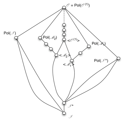
Figure 1. Monoidal intervals

The following theorem describes $I_{\mathscr{M}}$ for all monoids ${\mathscr{M}}$ which contain an operation which is neither injective nor constant. We refer the reader to Section 5, which contains the proof of the theorem, for the definition of quasilinearity.

Theorem 8.

Let ${\mathscr{M}}$ be a locally closed monoid containing $S_{\mathbb{N}}$ as well as a non-constant and non-injective operation. Then:

1. If ${\mathscr{M}}={\mathscr{O}}^{(1)}$, then $I_{\mathscr{M}}$ is a chain of order type $\omega+1$ with largest element ${\mathscr{O}}$.
   Its smallest element is the clone $\langle{\mathscr{O}}^{(1)}\rangle$ of all essentially unary operations.
   Its second smallest element is Burle’s clone ${\mathscr{Q}}$ of all operations which are either essentially unary or quasilinear.
   For $n\geq 3$, its $n$-th smallest element is the clone ${\mathscr{K}}_{n}$ of all operations which are either essentially unary or whose range contains less than $n$ elements.

2. If ${\mathscr{M}}\neq{\mathscr{O}}^{(1)}$, then there exists a maximal natural number $k=k({\mathscr{M}})\geq 1$ such that ${\mathscr{M}}$ contains all unary operations which take at most $k$ values.
   If $k=1$, then $I_{\mathscr{M}}$ has only one element $\langle{\mathscr{M}}\rangle$.
   Otherwise, $I_{\mathscr{M}}$ is a finite chain of length $k+1$, and:
   Its smallest element is $\langle{\mathscr{M}}\rangle$.
   Its second smallest element ${\mathscr{Q}}^{\mathscr{M}}$ consists of $\langle{\mathscr{M}}\rangle$ plus all quasilinear operations.
   For $3\leq n\leq k+1$, its $n$-th smallest element ${\mathscr{K}}^{\mathscr{M}}_{n}$ consists of $\langle{\mathscr{M}}\rangle$ plus all operations whose range is smaller than $n$.

We now turn to the monoid ${\mathscr{I}}$ locally generated by $S_{\mathbb{N}}$. This, as a quick check shows, consists of all injections in ${\mathscr{O}}^{(1)}$. Its monoidal interval is the hardest to understand, and we need a few definitions before stating the theorem describing it.

Definition 9 (The Horn clone ${\mathscr{H}}$).

Let ${\mathscr{H}}$ be the set of operations which are, up to fictitious variables, injective.

Definition 10 (The Bar clone ${\mathscr{B}}$).

Let $f\in{\mathscr{O}}^{(2)}$ and let $k\geq 1$. If there exists an injection $p\in{\mathscr{O}}^{(2)}$ such that $f(x_{1},x_{2})=p(x_{1},x_{2})$ for all $x_{1}\geq k$ and $f(x_{1},x_{2})=p(x_{1},0)=x_{1}$ for all $x_{1}<k$, then we call $f$ a $k$-bar function. Let ${\mathscr{B}}$ be the clone generated (in the sense of 3.1) by any bar function, i.e., the smallest local clone containing that bar function and all permutations of $\mathbb{N}$ (we will see in Section 6.2 that this definition makes sense).

Definition 11 (Richard ${\mathscr{R}}$).

Let $1\leq i\leq n$. We call an operation $f\in{\mathscr{O}}^{(n)}$ injective in the $i$-th direction iff $f(a)\neq f(b)$ whenever $a,b\in X^{n}$ and $a_{i}\neq b_{i}$. We say that $f\in{\mathscr{O}}^{(n)}$ is injective in one direction iff there exists $1\leq i\leq n$ such that $f$ is injective in the $i$-th direction. Let ${\mathscr{R}}$ be the set of all operations which are injective in one direction.

Definition 12 (The odd clone ${\mathscr{S}}$).

Let $f_{3}\in{\mathscr{O}}^{(3)}$ any operation satisfying the following:

• $f_{3}(x,1,1)=1$, $f_{3}(2,x,2)=2$, $f_{3}(3,3,x)=3$, and

• For all other arguments, the function arbitrarily takes a value that is distinct from all other function values.

We set ${\mathscr{S}}$ to be the clone generated by $f_{3}$, i.e., the smallest local clone containing $f_{3}$ and $S_{\mathbb{N}}$.

The following theorem summarizes the highlights of the monoidal interval corresponding to the monoid ${\mathscr{I}}$ generated by $S_{\mathbb{N}}$; confer Figure 2. More detailed descriptions of the clones of the theorem as well as other clones in that interval can be found in Section 6.

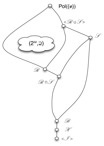
Figure 2. The monoidal interval of ${\mathscr{I}}$

Theorem 13.

The monoid locally generated by $S_{\mathbb{N}}$ is the monoid ${\mathscr{I}}$ of injections, and:

1. The largest element of $I_{\mathscr{I}}$, $\operatorname{Pol}({\mathscr{I}})$, equals $\operatorname{Pol}(\{\neq\})$, where $\neq$ is the (binary) inequality relation.

2. ${\mathscr{H}}$ is the unique cover of $\langle{\mathscr{I}}\rangle$ in $I_{\mathscr{I}}$, and all elements of $I_{\mathscr{I}}$ except $\langle{\mathscr{I}}\rangle$ contain ${\mathscr{H}}$. Moreover, ${\mathscr{H}}$ is generated by any binary injection, and $\operatorname{Inv}({\mathscr{H}})$ consists of all relations definable by a Horn formula.

3. ${\mathscr{B}}$ is the unique cover of ${\mathscr{H}}$ in $I_{\mathscr{I}}$, and all elements of $I_{\mathscr{I}}$ except $\langle{\mathscr{I}}\rangle$ and ${\mathscr{H}}$ contain ${\mathscr{B}}$.

4. ${\mathscr{R}},{\mathscr{S}}$ are incomparable clones in $I_{\mathscr{I}}$ and every clone in $I_{\mathscr{I}}$ is either contained in ${\mathscr{S}}$ or contains ${\mathscr{R}}$.

5. The number of elements of $I_{\mathscr{I}}$ containing ${\mathscr{R}}$ equals the continuum: In fact, the power set of $\omega$, ordered by reverse inclusion, has an order embedding into the interval $[{\mathscr{R}},\operatorname{Pol}({\mathscr{I}})]$. In particular, the same holds for the interval $I_{\mathscr{I}}$, as well as for the set of local clones above $S_{\mathbb{N}}$.

The last statement of Theorem 13 is among the hardest to prove in this paper, and has strong consequences for pp classification projects, so that it deserves an own corollary.

Corollary 14.

Let $\Gamma$ be any relational structure. Then the number of its pp-closed reducts is uncountable. In fact, there exists an order embedding of the power set of $\omega$ into the lattice of pp-closed reducts of $\Gamma$.

It is for this reason that we cannot expect to completely characterize the pp-closed reducts of any relational structure. In our case, we obtain a complete characterization of the closed monoid lattice and of all monoidal intervals except for those corresponding to the monoids ${\mathscr{I}}$ and ${\mathscr{I}}^{+}$ (see below), where we must content ourselves with some insights on the structure of those intervals.

It remains to describe the monoidal intervals of those monoids which contain all injections, and some constant operations. Clearly, there is only one such monoid, namely the monoid ${\mathscr{I}}^{+}$ consisting of all constants and all injections. In general, for any set of operations ${\mathscr{F}}\subseteq{\mathscr{O}}$, write ${\mathscr{F}}^{+}$ for ${\mathscr{F}}$ plus all constant operations, and ${\mathscr{F}}^{-}$ for ${\mathscr{F}}$ without all constant operations. It turns out that $I_{{\mathscr{I}}^{+}}$ is a complete sublattice of $I_{{\mathscr{I}}}$, as described in the following theorem:

Theorem 15.

Let ${\mathscr{I}}^{+}$ be the monoid of all injective and of all constant operations. Then:

1. If ${\mathscr{C}}\in I_{{\mathscr{I}}^{+}}$, then ${\mathscr{C}}^{-}$ is a local clone in $I_{\mathscr{I}}$.

2. $\langle{\mathscr{I}}^{+}\rangle^{-}=\langle{\mathscr{I}}\rangle$ and $(\operatorname{Pol}({\mathscr{I}}^{+}))^{-}={\mathscr{S}}$.

3. The mapping from $I_{{\mathscr{I}}^{+}}$ into the subinterval $[\langle{\mathscr{I}}\rangle,{\mathscr{S}}]$ of $I_{\mathscr{I}}$ which sends every clone ${\mathscr{C}}$ to ${\mathscr{C}}^{-}$ is a complete lattice embedding which preserves the smallest and the largest element.

4. If ${\mathscr{C}},{\mathscr{D}}\in I_{{\mathscr{I}}^{+}}$, then ${\mathscr{C}}\subsetneq{\mathscr{D}}$ iff ${\mathscr{C}}^{-}\subsetneq{\mathscr{D}}^{-}$.

5. For all ${\mathscr{C}}\in I_{\mathscr{I}}$ which do not contain ${\mathscr{R}}$, $\langle{\mathscr{C}}^{+}\rangle$ is a local clone in $I_{{\mathscr{I}}^{+}}$.

6. All clones ${\mathscr{C}}$ in $I_{{\mathscr{I}}^{+}}$ are of this form, as ${\mathscr{C}}=({\mathscr{C}}^{-})^{+}$.

7. $\langle{\mathscr{R}}^{+}\rangle={\mathscr{O}}$.

8. ${\mathscr{H}}^{+}$ is the unique cover of $\langle{\mathscr{I}}^{+}\rangle$ in $I_{{\mathscr{I}}^{+}}$.

9. ${\mathscr{B}}^{+}$ is the unique cover of ${\mathscr{H}}^{+}$ in $I_{{\mathscr{I}}^{+}}$.

We remark that the mapping that sends every ${\mathscr{C}}\in I_{{\mathscr{I}}^{+}}$ to ${\mathscr{C}}^{-}$ is not surjective onto the interval $[\langle{\mathscr{I}}\rangle,{\mathscr{S}}]$; see the remark after Proposition 85.

The following sections contain the proof of our result, and of course more detailed definitions of the structures involved. Each theorem corresponds to a section: Theorems $7$, $8$, $13$ and $15$ are proven in Sections $4$, $5$, $6$, and $7$, respectively.

3.1. Additional notation and terminology

In addition to the notation introduced so far, we establish the following conventions. If $f\in{\mathscr{O}}$, since we are only interested in local clones containing $S_{\mathbb{N}}$, we abuse the notation $\langle\cdot\rangle$ and write $\langle f\rangle$ for the local clone generated by $f$ together with $S_{\mathbb{N}}$. For $f,g\in{\mathscr{O}}$, we say that $f$ generates $g$ iff $g\in\langle f\rangle$. Similarly for $g\in{\mathscr{O}}$ and ${\mathscr{F}}\subseteq{\mathscr{O}}$, we say that ${\mathscr{F}}$ generates $g$ iff $g\in\langle{\mathscr{F}}\rangle$. If $f\in{\mathscr{O}}$, we write $\operatorname{ran}(f)$ for its range.

For a relation $R$, we will usually write $\operatorname{Pol}(R)$ instead of $\operatorname{Pol}(\{R\})$ for the set of all operations which preserve $R$. If $a$ is an $n$-tuple, then we refer by $a_{i}$ to the $i$-th component of $a$, for all $1\leq i\leq n$.

4. The basis: Monoids

We prove Theorem 7 describing all unary clones containing $S_{\mathbb{N}}$. Recall that a unary clone consists only of operations depending on at most one variable, and is therefore a disguised monoid of transformations. For convenience, we therefore only deal with unary operations and monoids in this section. In particular, we adjust the meaning of certain notations for this section: For example, $\langle{\mathscr{F}}\rangle$ refers to the local monoid (rather than the local clone) generated by a set ${\mathscr{F}}\subseteq{\mathscr{O}}^{(1)}$ together with $S_{\mathbb{N}}$.

The various statements of Theorem 7 are obtained in Propositions 26, 30, 32 and Corollaries 27 and 31.

In a first lemma, we officially state what we already observed in the last section, namely that $S_{\mathbb{N}}$ locally generates all unary injections.

Lemma 16.

Let ${\mathscr{M}}\supseteq S_{\mathbb{N}}$ be a locally closed monoid. Then ${\mathscr{M}}$ contains the monoid ${\mathscr{I}}$ of all unary injective operations.

Proof.

Clearly, on any finite set every injection can be locally interpolated by a suitable permutation. ∎

The following lemma implies that except for the full transformation monoid ${\mathscr{O}}^{(1)}$, all closed monoids above $S_{\mathbb{N}}$ consist of the injections plus some finite range operations.

Lemma 17.

Let $f\in{\mathscr{O}}^{(1)}$ have infinite image, and assume it is not injective. Then $f$ generates all unary operations.

Proof.

We skip the fairly easy proof, and refer the reader to the very similar (first part of the) proof of Lemma 20. ∎

We thus wish to know, given a finite range operation, which other finite range operations it generates. For that, we need the following concept.

Definition 18.

Let $f\in{\mathscr{O}}^{(1)}$ have finite range, and write $n=|\operatorname{ran}(f)|$. Enumerate the kernel classes of $f$ by $C_{1},\ldots,C_{n}$ in such a way that their sizes are increasing. The kernel tuple $\kappa^{f}\in(\omega+1)^{n}$ of $f$ is the $n$-tuple $(|C_{1}|,\ldots,|C_{n}|)$.

Note that the last entry of a kernel tuple $\kappa^{f}$ always equals $\omega$ since $f$ must have at least one infinite kernel class.

Having assigned a finite sequence with positive values in $\omega+1$ to every finite range operation, we are ready to order such sequences and give the definition of $\mathbb{P}$.

Definition 19.

• Let $k,n\geq 1$. For $a\in(\omega+1)^{k}$ and $b\in(\omega+1)^{n}$ we write $a\sqsubseteq b$ iff $k\leq n$ and the following holds: There exists a partition $\{A_{1},\ldots,A_{k}\}$ of $\{1,\ldots,n\}$ into $k$ classes such that $a_{i}\leq\sum_{j\in A_{i}}b_{j}$ for all $1\leq i\leq k$.

• We write $\mathbb{P}_{\infty}$ for the partial order of finite increasing sequences of non-zero elements of $\omega+1$ ordered by $\sqsubseteq$.

• We write $\mathbb{P}$ for the partial order of the finite increasing sequences of positive natural numbers (not of values in $\omega+1$!) ordered by $\sqsubseteq$.

Observe that for finite increasing sequences $a,b\in(\omega+1)^{n}$ of the same length we have $a\sqsubseteq b$ iff $a_{i}\leq b_{i}$ for all $1\leq i\leq n$. The following lemma justifies our definition of $\sqsubseteq$.

Lemma 20.

Let $f,g\in{\mathscr{O}}^{(1)}$ have finite range. Then $f$ generates $g$ iff $\kappa^{g}\sqsubseteq\kappa^{f}$.

Proof.

Assume first that $\kappa^{g}\sqsubseteq\kappa^{f}$. Let $\kappa^{f}$ have length $n$ and $\kappa^{g}$ have length $k\leq n$. If $k=n$, then $\kappa^{g}_{i}\leq\kappa^{f}_{i}$ for all $1\leq i\leq n$. It is then not hard to see that for any finite set $A\subseteq\mathbb{N}$, there exist permutations $\alpha,\beta$ such that $\beta\circ f\circ\alpha$ agrees with $g$ on $A$. If $k<n$, then let $A_{1},\ldots,A_{k}$ be the partition provided by the definition of $\sqsubseteq$. Enumerate the kernel classes of $f$ by $C_{1},\ldots,C_{n}$ and in such a way that $C_{j}$ contains $\kappa^{f}_{j}$ elements, for all $1\leq j\leq n$. Now take any $i,j\in\{1,\ldots,n\}$ which are distinct but equivalent with respect to the partition $A_{1},\ldots,A_{k}$. By composing $f$ with a permutation, we may assume that $f$ maps the classes $C_{i}$ and $C_{j}$ into the class $C_{n}$, and all other classes into classes $\neq C_{n}$ in such a way that no two classes are mapped into the same class. Then $t_{n-1}:=f\circ f$ is a function with $n-1$ values in its range, and $\kappa^{g}\sqsubseteq\kappa^{t_{n-1}}$. Proceeding like this, we arrive after $n-k$ steps at an operation $t_{k}$ which takes $k$ values and which satisfies $\kappa^{g}_{i}\leq\kappa^{t_{k}}_{i}$ for all $1\leq i\leq k$. Thus we are back in the case $k=n$, and the proof of this direction of the lemma is finished.

For the other direction, assume that $f$ generates $g$. Let $k,n$ be as before. Since the local clone generated by $f$ is the topological closure of the set of term operations generated by $f$, we have that for every $q\in\mathbb{N}$, there exists a term $t_{q}$ consisting of permutations and $f$ which agrees with $g$ on the finite set $\{0,\ldots,q\}$. We can write each $t_{q}$ as $t_{q}=s_{q}\circ f\circ\alpha_{q}$, where $s_{q}$ consists of permutations and $f$, and $\alpha_{q}$ is a permutation. Thus in every term $t_{q}$, certain classes of $f$ are joined by the application of $s_{q}$ (and shifted by $\alpha_{q}$, which we do not care about for the moment); since there are only finitely many possibilities of joining classes of $f$, there is one constellation which appears for infinitely many $q$. Since $q\leq q^{\prime}$ implies that $t_{q^{\prime}}$ agrees with $g$ on $\{0,\ldots,q\}$, by replacing terms we may assume that the same classes are joined for all $q\in\mathbb{N}$. Naturally, this partition of classes induces a partition $A_{1},\ldots,A_{w}$ on $\{1,\ldots,n\}$ via $\kappa^{f}$. If $p,r\leq q$ are equivalent modulo the kernel of $g$, then the kernel classes of $f$ containing $\alpha_{q}(p)$ and $\alpha_{q}(r)$, respectively, are equivalent with respect to the partition $A_{1},\ldots,A_{w}$. On the other hand, if $p,r\leq q$ are not in the same class of $g$, then $\alpha_{q}(p)$ and $\alpha_{q}(r)$ will not lie in equivalent $f$-classes. Thus, taking $q$ large enough so that $\{0,\ldots,q\}$ meets all kernel classes of $g$, we can assign to every $g$-class (with, say, index $1\leq u\leq k$) an equivalence class $A_{e}\in\{A_{1},\ldots,A_{w}\}$ in an injective way; in particular, $k\leq w$. For infinitely many $q$, this assignment is the same; again, by replacing terms where necessary, we may assume it is always the same. Since for large enough $q$ arbitrarily large parts of the kernel classes of $g$ are hit, we must have $\kappa^{g}_{u}\leq\sum_{j\in A_{e}}\kappa^{f}_{j}$ for all $1\leq u\leq k$, where $A_{e}$ is the class assigned to $u$. By joining some classes $A_{i}$, we can obtain $w=k$ without changing the latter fact. ∎

Lemma 21.

Let ${\mathscr{F}}\subseteq{\mathscr{O}}^{(1)}$. If there is no finite bound to the sizes of the ranges of the finite range operations in ${\mathscr{F}}$, then ${\mathscr{F}}$ generates ${\mathscr{O}}^{(1)}$.

Proof.

Let $f$ be any finite range operation, and let $A\subseteq\mathbb{N}$ be finite. Then there exists a finite range function $g$ which agrees with $f$ on $A$ and whose kernel sequence $\kappa^{g}$ has only one entry equal to $\omega$. Now there exists a finite range operation $h$ in ${\mathscr{F}}$ with $\kappa^{g}\sqsubseteq\kappa^{h}$, so $g$ is generated by ${\mathscr{F}}$. This proves that $f$ is generated by ${\mathscr{F}}$, and hence ${\mathscr{F}}$ generates all finite range operations. Clearly, any operation in ${\mathscr{O}}^{(1)}$ can be interpolated on any finite set by a finite range operation, which implies our assertion. ∎

The following is a consequence of Lemma 20; it says that if finitely many finite range operations join forces, the joint generating power is not more than the sum of the generating powers of the single operations.

Proposition 22.

Let ${\mathscr{F}}\subseteq{\mathscr{O}}^{(1)}$ be finite. Then $\langle{\mathscr{F}}\rangle=\bigcup\{\langle f\rangle:f\in{\mathscr{F}}\}$.

Proof.

The non-trivial direction is to show $\langle{\mathscr{F}}\rangle\subseteq\bigcup\{\langle f\rangle:f\in{\mathscr{F}}\}$. If $t$ is any term made of operations in ${\mathscr{F}}$, then it is of the form $r\circ f$, where $r$ is a term and $f\in{\mathscr{F}}$. Clearly, $\kappa^{t}\sqsubseteq\kappa^{f}$, implying $t\in\langle\{f\}\rangle$. Thus, $\bigcup\{\langle f\rangle:f\in{\mathscr{F}}\}$ contains all terms that can be built from ${\mathscr{F}}$. This implies that the union is a monoid. Being a finite union of (topologically) closed sets $\bigcup\{\langle f\rangle:f\in{\mathscr{F}}\}$ is itself closed, and hence contains even $\langle{\mathscr{F}}\rangle$. ∎

We now assign ideals of $\mathbb{P}$ to local monoids containing $S_{\mathbb{N}}$.

Definition 23.

For a local monoid ${\mathscr{M}}\supseteq S_{\mathbb{N}}$, we set

$$\operatorname{Id}_{\infty}({\mathscr{M}})=\{\kappa^{f}:f\in{\mathscr{M}},\,f\mbox{ has finite range}\}\subseteq\mathbb{P}_{\infty}.$$

For a sequence $s\in\mathbb{P}$, write $s\ast\infty\in\mathbb{P}_{\infty}$ for the sequence obtained by gluing $\omega$ to the end of $s$. Now set

$$\operatorname{Id}({\mathscr{M}})=\{s\in\mathbb{P}:s\ast\infty\in\operatorname{Id}_{\infty}({\mathscr{M}})\}.$$

By Lemma 20, $\operatorname{Id}({\mathscr{M}})$ is always an ideal of $\mathbb{P}$. Conversely, we show in the following how to get closed monoids from ideals of $\mathbb{P}$.

Definition 24.

Let $k\geq 1$ and let $(s^{n})_{n\in\omega}$ be an ascending sequence of $k$-tuples in $\mathbb{P}_{\infty}$. We write $\lim_{n}(s^{n})$ for the smallest (according to $\sqsubseteq$) $k$-tuple $s$ in $\mathbb{P}_{\infty}$ satisfying $s^{n}\sqsubseteq s$ for all $n\in\omega$.
For an ideal $I\subsetneq\mathbb{P}$, we let $\operatorname{Mon}(I)$ contain all operations in ${\mathscr{O}}^{(1)}$ which are either injective, or which have finite range and whose kernel sequence is a limit of an ascending sequence of $k$-tuples of the form $s\ast\infty$, where $s\in I$.

Lemma 25.

Let $I\subsetneq\mathbb{P}$ be an ideal. Then $\operatorname{Mon}(I)$ is a local monoid containing $S_{\mathbb{N}}$.

Proof.

Observe that if $f\in\operatorname{Mon}(I)$ is a finite range function, and if $g\in{\mathscr{O}}^{(1)}$ is a finite range function such that $\kappa^{g}\sqsubseteq\kappa^{f}$, then $\operatorname{Mon}(I)$ contains also $g$. For, let the range of $f$ have $n$ elements, let the range of $g$ have $k\leq n$ elements, and let $A_{1},\ldots,A_{k}$ be the partition of $\{1,\ldots,n\}$ provided by the definition of $\sqsubseteq$. A quick check shows that we may assume $A_{k}=\{n\}$. Let $(s^{i})_{i\in\omega}$ be the sequence of $(n-1)$-tuples in $I$ such that $\lim_{i}(s^{i}\ast\infty)=\kappa^{f}$. Set $t^{i}_{j}:=\sum_{r\in A_{j}}s^{i}_{r}$, for all $i\in\omega$ and all $1\leq j\leq k-1$. Since $t^{i}\sqsubseteq s^{i}$, all $t^{i}$ are elements of $I$, provided they are actually increasing tuples. Fixing $i$, define inductively $w^{i}_{j}:=\max\{t^{i}_{r}:r\leq j\}$, for all $1\leq j\leq k-1$. It is not hard to see that the $w^{i}$ are in $I$, too, and that $\kappa^{g}$ is the limit of the increasing sequence $(w^{i}\ast\infty)_{i\in\omega}$, so $g\in\operatorname{Mon}(I)$.

Using Lemma 20 and Proposition 22, one now readily derives from this that $\operatorname{Mon}(I)$ is indeed a monoid. It remains to show that $\operatorname{Mon}(I)$ is local. Let $f\in{\mathscr{O}}^{(1)}$, and assume it can be interpolated on all finite sets by operations from $\operatorname{Mon}(I)$; assume also that it is not injective. If $f$ has infinite range, then $\operatorname{Mon}(I)$ must contain non-injections of arbitrarily large finite range, which in turn implies that $I$ contains tuples of arbitrary length. The definition of $\mathbb{P}$ then shows that $I=\mathbb{P}$, a contradiction. Thus, all non-injections in the local closure of $\operatorname{Mon}(I)$ have finite range. Assume again that $f$ is such a non-injection, and assume $\kappa^{f}$ has length $k$. Fix for every set $\{0,\ldots,n\}$ an operation $f_{n}\in\operatorname{Mon}(I)$ which agrees with $f$ on this set. From some $n$ on, the $f_{n}$ will have to take at least $k$ values, so we take the liberty of assuming that all $f_{n}$ have this property. An easy manipulation of the $f_{n}$ using the fact that $g\in\operatorname{Mon}(I)$ whenever $\kappa^{g}\sqsubseteq\kappa^{f_{n}}$ allows us to assume that every $f_{n}$ takes exactly $k$ values and that $\kappa^{f_{n}}\sqsubseteq\kappa^{f}$ for all $n\in\omega$. By thinning out the sequence, we may also assume that the kernel sequences of the $f_{n}$ are increasing with respect to $\sqsubseteq$. We then have $\lim_{n}(\kappa^{f_{n}})=\kappa^{f}$. Now replace each $k$-tuple $\kappa^{f_{n}}$ by a $(k-1)$-tuple $s^{n}\in\mathbb{P}$ with $s^{n}\ast\infty\sqsubseteq\kappa^{f_{n}}$ in such a way that $\lim_{n}(s^{n}\ast\infty)=\lim_{n}(\kappa^{f_{n}})$ and that the sequence $(s^{n})_{n\in\omega}$ is still ascending. Clearly, $s^{n}\in I$ for all $n\in\omega$, and so $\kappa^{f}=\lim_{n}s^{n}$ implies $f\in\operatorname{Mon}(I)$. Hence, $\operatorname{Mon}(I)$ is locally closed. ∎

Proposition 26.

The mapping $\sigma:{\mathscr{M}}\mapsto\operatorname{Id}({\mathscr{M}})$ is an isomorphism from the lattice ${\mathfrak{U}}$ of locally closed monoids that contain $S_{\mathbb{N}}$ onto the lattice of ideals of $\mathbb{P}$.

Proof.

That $\operatorname{Id}({\mathscr{M}})$ is an ideal of $\mathbb{P}$ for all monoids ${\mathscr{M}}$ follows directly from Lemma 20. From Lemma 21 we know that $\operatorname{Id}({\mathscr{M}})=\mathbb{P}$ iff ${\mathscr{M}}={\mathscr{O}}^{(1)}$, and obviously $\operatorname{Id}({\mathscr{M}})=\emptyset$ iff ${\mathscr{M}}$ contains only injections. We have seen in Lemma 25 that for any proper ideal $I$ of $\mathbb{P}$, $\operatorname{Mon}(I)$ is a local monoid, and a straightforward verification shows $\operatorname{Id}(\operatorname{Mon}(I))=I$, thus $\sigma$ is onto. Also, an easy check using Lemma 20 shows that $\operatorname{Mon}(\operatorname{Id}({\mathscr{M}}))={\mathscr{M}}$ for every local monoid which contains $S_{\mathbb{N}}$ and all of whose non-injections have finite range, so $\sigma$ is injective. It is obvious that both $\sigma$ and $\sigma^{-1}$ are order-preserving. ∎

Recall that a lattice is algebraic iff it is isomorphic to the subalgebra lattice of an algebra.

Corollary 27.

The lattice ${\mathfrak{U}}$ of local monoids above $S_{\mathbb{N}}$ is distributive. Moreover, ${\mathfrak{U}}$ and its dual order are algebraic.

Proof.

By the preceding proposition, ${\mathfrak{U}}$ is the lattice of ideals of a partial order. The assertions then follow from [CD73, p. 83]. ∎

Definition 28.

A partial order is called a well-quasi-order iff there are no infinite descending chains and no infinite antichains in it.
We call a sequence $(a^{n})_{n\in\omega}$ in a partial order with order relation $\leq$ bad iff for no $i<j\in\omega$ we have $a^{i}\leq a^{j}$.

A standard application of the infinite Ramsey’s theorem shows that a partial order is well-quasi-ordered iff it contains no bad sequence (confer e.g. [Die05]).

Lemma 29.

The set of finite sequences with values in $\omega+1$ ordered by $\sqsubseteq$ is a well-quasi-order. In particular, its suborders $\mathbb{P}_{\infty}$ and $\mathbb{P}$ are well-quasi-orders.

Proof.

Assume that $(a^{n})_{n\in\omega}$ were a bad sequence of such finite sequences. For every $n\in\omega$, let $w_{n}$ be the number of occurrences of $\omega$ in the tuple $a^{n}$. If the sequence $(w_{n})_{n\in\omega}$ were unbounded, then we could find $n\in\omega$ such that $w_{n}$ is greater than the length of $a^{0}$, implying $a^{0}\sqsubseteq a^{n}$, a contradiction. Thus, we can thin out the sequence in such a way that all $w_{n}$ are equal. Let $b^{n}$ be the tuple obtained from $a^{n}$ by leaving away the $w_{n}$ components equal to $\omega$, for all $n\in\omega$. Clearly, the $b^{n}$ form a bad sequence of tuples with values in $\omega$. Now if the sequence of lengths of the $b^{n}$ were unbounded, then we could find some $i\in\omega$ such that the length of $b^{i}$ is greater than the sum of all components of $b^{0}$, hence $b^{0}\sqsubseteq b^{i}$, a contradiction. Thin out the sequence $(b^{n})_{n\in\omega}$ is such a way that all tuples have the same length $k$. Now for all $1\leq j\leq k$, we thin out our sequence so that the sequence consisting of the $j$-th component of the $b^{n}$ is increasing; we can do this since $\omega$ is well-ordered. The remaining sequence of $b^{n}$ is ascending, a contradiction. ∎

In general, the ideal lattice of a given well-quasi-order need not be a well-quasi-order. Certain well-quasi-orders which satisfy a certain strong combinatorial property and which are called better-quasi-orders, however, do have the property that their ideal lattice is well-quasi-ordered. Although giving the definition of a better-quasi-order (see e.g. [Mil85]) would be out of scope of the present paper, we remark that it follows from the basic theory of better-quasi-orders that our well-quasi-order $\mathbb{P}$ is in fact a better-quasi-order (as Kruskal states in [Kru72]: “All naturally known well-quasi-ordered sets which are known are better-quasi-ordered.”). Therefore, the lattice of ideals of $\mathbb{P}$ is a well-quasi-order (and, in fact, even a better-quasi-order as well). In order to spare the reader the pain of reading the definition of a better-quasi-order, we prove the following

Proposition 30.

The lattice of ideals of $\mathbb{P}$ is a well-quasi-order.

Proof.

Suppose that $(I_{n})_{n\in\omega}$ were a bad sequence of ideals. By taking away the first element of the sequence, we may assume that $I_{n}\neq\mathbb{P}$ for all $n\in\omega$. Consider for all $n\in\omega$ the set $J_{n}$ consisting of $I_{n}$ plus all limits of ascending chains of tuples of the same length in $I_{n}$ (as in Definition 24): So $J_{n}\subseteq\mathbb{P}_{\infty}$ for all $n\in\omega$. In $J_{n}$, every chain is bounded from above: If $C$ is a chain in $J_{n}$, then there is some $k\in\omega$ such that all tuples in $C$ have length at most $k$; for otherwise, $I_{n}$ contains sequences of arbitrary length, implying $I_{n}=\mathbb{P}$ contrary to our assumption. But if the elements of $C$ all have length at most $k$, then $C$ is bounded by construction of $J_{n}$ (i.e., adding the limits of ascending chains).

Applying Zorn’s lemma, we get that every element of $I_{n}$ is below some maximal tuple of $J_{n}$. By construction of $J_{n}$, every tuple in $\mathbb{P}$ which is below a maximal tuple of $J_{n}$ also is an element of $I_{n}$. The maximal elements of $J_{n}$ form an antichain with respect to $\sqsubseteq$. By Lemma 29, the set of sequences in $\omega+1$, equipped with the order $\sqsubseteq$, is a well-quasi-order. In particular, the antichain of maximal elements of $J_{n}$ is finite. For every $n>0$, there exists a tuple in $I_{0}\setminus I_{n}$. Thus, there is a maximal tuple of $J_{0}$ which is not in $J_{n}$. We can thin out our sequence of $I_{n}$ so that this witnessing maximal tuple is the same for all $n>0$; denote it by $s^{0}$. Now we do the same for $J_{1}$ and all $n>1$, obtaining a maximal tuple $s^{1}\in J_{1}$ which is not in any $J_{n}$ with $n>1$. We continue inductively in this fashion, obtaining a sequence $(s^{n})_{n\in\omega}$. By construction, this sequence is a bad sequence in the order of finite $(\omega+1)$-valued sequences with $\sqsubseteq$, a contradiction. ∎

Corollary 31.

The lattice of local monoids above $S_{\mathbb{N}}$ is well-quasi-ordered.

Proposition 32.

Every local monoid ${\mathscr{M}}$ above $S_{\mathbb{N}}$ is finitely generated over $S_{\mathbb{N}}$, i.e., there exists a finite ${\mathscr{F}}\subseteq{\mathscr{O}}^{(1)}$ such that ${\mathscr{M}}=\langle{\mathscr{F}}\rangle$. Moreover, the number of such monoids is countable.

Proof.

If ${\mathscr{M}}={\mathscr{O}}^{(1)}$, then it is generated by any non-injective operation with infinite range, by Lemma 17. Assume henceforth that ${\mathscr{M}}$ contains only injections and finite range operations. Set $J$ to consist of all kernel sequences of operations in ${\mathscr{M}}$. By local closure and what is by now a standard argument, one sees that every chain in $J$ has an upper bound in $J$ (confer e.g. the proof of Lemma 25). Hence, Zorn’s lemma implies that every element of $J$ is below a maximal element of $J$. The maximal elements of $J$ form an antichain with respect to $\sqsubseteq$, and therefore are finite in number by Lemma 29. Pick for each maximal tuple one corresponding operation in ${\mathscr{M}}$. The set ${\mathscr{F}}$ of operations thus chosen is as desired, by Lemma 20.

The above argument shows that every local monoid containing $S_{\mathbb{N}}$ is determined by a finite set of finite sequences with values in $\omega+1$. There are only countably many possibilities for such finite sets, so the number of such monoids is countable. ∎

5. Clones with essential finite range operations

Having understood the structure of the lattice of local monoids containing $S_{\mathbb{N}}$, we move on to describe the monoidal interval corresponding to each such monoid. In this section, we will prove Theorem 8, which deals with those monoids which contain a non-constant and non-injective operation.

Definition 33.

An operation $f$ on a set $Y$ is called essential iff it is not essentially unary, i.e., it depends on at least two of its variables.

We will see that except for ${\mathscr{O}}$, all clones whose unary fragment contains a non-constant and non-injective operation contain only essential operations with finite range, and none with infinite range; hence the title of this section.

It turns out that the monoidal intervals of the monoids under consideration here are all chains which can be described nicely. This is essentially a consequence of a theorem from [HR94] for clones on finite sets, and the power of local closure. In order to state that theorem, we need the following definition.

Definition 34.

Let $Y$ be any set. We call an $n$-ary operation $f$ on $Y$ quasilinear iff there exist functions $\phi_{0}:\{0,1\}\rightarrow Y$ and $\phi_{1},\ldots,\phi_{n}:Y\rightarrow\{0,1\}$ such that $f(x_{1},\ldots,x_{n})=\phi_{0}(\phi_{1}(x_{1})\dot{+}\ldots\dot{+}\phi_{n}(x_{n}))$, where $\dot{+}$ denotes the sum modulo $2$.

Theorem 35 ([HR94]).

Let $Y$ be a finite set of at least three elements and let $f$ be an essential operation on $Y$. Set $k:=|\operatorname{ran}(f)|$. Then, writing $S_{Y}$ for the set of all permutations on $Y$, we have:

• If $k\geq 3$, then $f$ together with $S_{Y}$ generate all operations on $Y$ which take at most $k$ values.

• If $k=2$ and $f$ is not quasilinear, then $f$ together with $S_{Y}$ generate all operations on $Y$ which take at most two values.

• If $k=2$, $f$ is quasilinear, and $|Y|$ is odd, then $f$ together with $S_{Y}$ generate all quasilinear operations on $Y$.

Observe that there is no such thing as local interpolation on finite $Y$, so “generates” in the theorem refers to the term closure.

The following lemma is the infinite local version of this theorem.

Lemma 36.

Let $f\in{\mathscr{O}}^{(n)}$ be essential, and assume that $|\operatorname{ran}(f)|=k$, where $2\leq k<\omega$.

1. If $k\geq 3$, then $f$ generates all operations which take at most $k$ values.

2. If $k=2$ and $f$ is not quasilinear, then $f$ generates all functions which take at most $k$ values.

3. If $k=2$ and $f$ is quasilinear, then $f$ generates all quasilinear operations.

Proof.

(1): Let any operation $g$ on $|\operatorname{ran}g|\leq k$ be given. It suffices to show that for every $n\in\omega$, $f$ generates an operation $h$ which agrees with $g$ on $\{0,\ldots,n\}$. Choosing $n$ large enough, we may assume that the ranges of both $f$ and $g$ are contained in $\{0,\ldots,n\}$. Also, again by making $n$ larger, we may assume that the restriction $f^{\prime}$ of $f$ to $\{0,\ldots,n\}$ is essential and takes $k$ values. Then $f^{\prime}$ is an essential operation on $\{0,\ldots,n\}$ which takes $k$ values, and hence generates all such functions by Theorem 35. In particular, $f^{\prime}$ generates a function $h^{\prime}$ which agrees with $g$ on $\{0,\ldots,n\}$. The permutations which appear in the term which represents $h^{\prime}$ can be extended to $X$ by the identity; occurrences of $f^{\prime}$ can be replaced by $f$. The resulting term $h$ is a function on $X$ which still agrees with $g$ on $\{0,\ldots,n\}$.
(2): Again, let $g$ and $n$ be given. Enlarge $n$ as before, if necessary, so that the restriction of $f$ to $\{0,\ldots,n\}$ is not quasilinear. Now we argue as in the preceding proof.
(3): The proof works as before; $n$ only has to be chosen odd in order to allow application of Theorem 35. ∎

With the preceding lemma, we see that it is quite easy to understand what happens when we add an essential finite range operation to a monoid. We will now show that to the monoids relevant for this section, we in fact cannot add an essential infinite range operation without generating ${\mathscr{O}}$. To establish this, we distinguish between those operations which preserve the binary inequality relation $\neq$, and those which do not. The latter case can be eliminated right away:

Proposition 37.

Let $f$ be an essential operation with infinite image. Then $f$ preserves $\neq$, or it generates all operations.

The proposition will follow from the following lemma.

Lemma 38.

Let $f\in{\mathscr{O}}^{(n)}$ have infinite image, and assume it does not preserve $\neq$. Then $f$ generates a unary non-injective function that has infinite range.

Before proving the lemma we show how the proposition follows from it:

Proof of Proposition 37.

By Lemma 38, $f$ generates a unary non-injective operation with infinite range; Lemma 17 then implies that $f$ generates all unary operations. Let $k\geq 1$ be arbitrary. We can find a unary finite range operation $g_{k}$ such that $g_{k}(f)$ is essential and takes at least $k$ values. By Lemma 36, this implies that $f$ generates all operations which take not more than $k$ values. Since $k$ was arbitrary and by local interpolation, this implies that $f$ generates ${\mathscr{O}}$. ∎

Proof of Lemma 38.

We only have to prove something if $f$ is essential, for $f$ is itself a unary non-injective operation with infinite range otherwise. We also assume $f$ to depend on all of its variables.
Case 1: There exist injective functions $g_{1},\ldots,g_{n}\in{\mathscr{O}}^{(1)}$ such that $f(g_{1},\ldots,g_{n})$ is injective. Choose $S\subseteq X$ infinite such that $X{\setminus}S$ and $X{\setminus}(g_{1}[S]\cup\ldots\cup g_{n}[S])$ are infinite. Since $f$ does not preserve $\neq$, there exist $c,d\in X^{n}$ such that $c_{i}\neq d_{i}$ for all $1\leq i\leq n$ and such that $f(c)=f(d)$. We may assume that those values are not in $S\cup g_{1}[S]\cup\ldots\cup g_{n}[S]$. For all $1\leq i\leq n$, set $g_{i}^{\prime}=g_{i}$ on $S$ and $g_{i}^{\prime}(c_{1})=c_{i}$ and $g_{i}^{\prime}(d_{1})=d_{i}$. Write $T=S\cup\{c_{1},d_{1}\}$. On $T$, $F=f(g_{1}^{\prime},\ldots,g_{n}^{\prime})$ is a function with infinite range which is not injective. Furthermore, the $g_{i}^{\prime}$ can be extended to permutations on $X$ since they are injective and have co-infinite domains and ranges. This completes the first case.
Case 2: $f(g_{1},\ldots,g_{n})$ is not injective for all injective $g_{1},\ldots,g_{n}\in{\mathscr{O}}^{(1)}$. Since $f$ is not constant, there exist injections $u_{1},\ldots,u_{n}\in{\mathscr{O}}^{(1)}$ such that $f(u_{1},\ldots,u_{n})$ is not constant. By assumption for this case we have that $f(u_{1},\ldots,u_{n})$ is not injective. Thus, $f(u_{1},\ldots,u_{n})$ generates a function $r\in{\mathscr{O}}^{(1)}$ which is constant except for one argument, at which it takes another value. To see this, just observe that for such an $r$, the kernel sequence $\kappa^{r}$ satisfies $\kappa^{r}\sqsubseteq\kappa^{h}$ for any non-constant $h\in{\mathscr{O}}^{(1)}$, and apply Lemma 20. Consider arbitrary $g_{1},\ldots,g_{n}\in{\mathscr{O}}^{(1)}$ such that $f(g_{1},\ldots,g_{n})$ is injective. Such functions exist since $f$ has infinite range. Pick an infinite $S\subseteq X$ on which each $g_{i}$ is either injective or constant. Observe that it is impossible that all those restrictions of $g_{i}$ are constant. Say the restriction of $g_{i}$ to $S$ is constant with value $c_{i}$ for $1\leq i\leq k$, where $1\leq k<n$.
Since $f$ depends on its first variable, there exist $c_{k+1},\ldots,c_{n}\in X$ and $a_{1},\ldots,a_{k}\in X$ such that $f(a_{1},\ldots,a_{k},c_{k+1},\ldots,c_{n})\neq f(c)$. For otherwise the value of $f$ is determined by the values of the arguments $x_{k+1},\ldots,x_{n}$, contradicting that $f$ depends on $x_{1}$. Choose $d_{k+1},\ldots,d_{n}\in X$ such that $f(c_{1},\ldots,c_{k},d_{k+1},\ldots,d_{n})$ is distinct from both $f(a_{1},\ldots,a_{k},c_{k+1},\ldots,c_{n})$ and $f(c)$; this is possible as $F(x_{k+1},\ldots,x_{n})=f(c_{1},\ldots,c_{k},x_{k+1},\ldots,x_{n})$ takes infinitely many values. Set $u_{i}(0)=a_{i}$ and $u_{i}(x)=c_{i}$ if $x\neq 0$, for $1\leq i\leq k$. Let moreover $v_{i}(1)=d_{i}$, and $v_{i}(x)=c_{i}$ if $x\neq 1$, for all $k+1\leq i\leq n$. All $u_{i}$ and $v_{i}$ are generated by the two-valued function $r$ and hence by $f$. Set $F(x)=f(u_{1},\ldots,u_{k},v_{k+1},\ldots,v_{n})(x)$. We have that $F(0)=f(a_{1},\ldots,a_{k},c_{k+1},\ldots,c_{n})$ and $F(1)=f(c_{1},\ldots,c_{k},d_{k+1},\ldots,d_{n})$ and $F(2)=f(c)$ are pairwise distinct; also, $F$ has finite range. Hence, $f$ generates a unary function $F$ that takes exactly three values.
Pick $a,b\in X^{n}$ such that $a_{i}\neq b_{i}$ for all $1\leq i\leq n$ and such that $f(a)=f(b)$. For all $1\leq i\leq k$, let $h_{i}\in{\mathscr{O}}^{(1)}$ satisfy $h_{i}(0)=a_{i}$, $h_{i}(1)=b_{i}$, and $h_{i}(x)=c_{i}$ for all $x\notin\{0,1\}$. Clearly, $h_{i}$ is generated by the unary function $F$ with three values, and hence also by $f$. For all $k+1\leq i\leq n$, let $\alpha_{i}$ be any permutation that maps $0$ to $a_{i}$ and $1$ to $b_{i}$. Now we set $G(x)=f(h_{1}(x),\ldots,h_{k}(x),\alpha_{k+1}(x),\ldots,\alpha_{n}(x))$ and have that $G(0)=f(a)=f(b)=G(1)$ and $G$ takes infinitely many values. ∎

We are thus left with essential infinite range operations which do preserve the inequality relation. The crucial theorem here has been shown in [BK08a].

Theorem 39.

Every essential operation $f\in\operatorname{Pol}(\neq)$ generates a binary injective operation.

Able to produce a binary injection, we use this operation in order to enlarge ranges of unary operations:

Lemma 40.

Let $f\in{\mathscr{O}}^{(2)}$ be injective, and let $g\in{\mathscr{O}}$ be a non-constant function with finite range. Then $f$ and $g$ together generate ${\mathscr{O}}$.

Proof.

Write $k:=|\operatorname{ran}(g)|$. Either $g$ is itself (essentially) unary, or it generates a non-constant unary operation which takes $k$ values by Lemma 36. Pick such a unary operation $g_{0}$, and set $k_{0}:=k$. The operation $t(x,y):=f(g(x),g(y))$ takes $k_{1}:=(k_{0})^{2}$ values. Hence, $f$ and $g$ together also generate a unary operation $g_{1}$ which takes $k_{1}$ values. Continuing in this fashion, and since $k_{0}=k>1$, we obtain unary operations of all finite ranges, and hence also ${\mathscr{O}}^{(1)}$ by Lemma 20. But clearly, for every operation $h\in{\mathscr{O}}^{(2)}$, there exists a unary $h^{\prime}\in{\mathscr{O}}^{(1)}$ such that $h(x,y)=h^{\prime}(f(x,y))$. Thus, since $h$ was arbitrary, $f$ and $g$ generate ${\mathscr{O}}^{(2)}$, and in turn also ${\mathscr{O}}$, as it is well-known and easy to see that $\langle{\mathscr{O}}^{(2)}\rangle={\mathscr{O}}$. ∎

We are thus ready to prove Theorem 8.

Proof of Theorem 8.

We are given a monoid ${\mathscr{M}}$ which contains an operation which is neither constant nor injective. It follows from Lemma 40 that no clone properly contained in ${\mathscr{O}}$ and containing ${\mathscr{M}}$ can have a binary injection. Therefore, by Theorem 39, it cannot have any essential operation which preserves the inequality relation. Nor can it contain an essential operation with infinite range which does not preserve the inequality, by Proposition 37. Thus, it cannot contain any essential operation with infinite range. We now distinguish the two cases of the theorem:
(1): If ${\mathscr{M}}={\mathscr{O}}^{(1)}$, then the only clones above ${\mathscr{O}}^{(1)}$ can be the ones mentioned in the theorem, by Lemma 36. That these sets of operations are actually clones is a straightforward verification and left to the reader.
(2): If ${\mathscr{M}}\neq{\mathscr{O}}^{(1)}$, then there is a largest natural number $k$ such that ${\mathscr{M}}$ contains all unary operations which take at most $k$ values; this follows from Lemma 21. If $k=1$, then no clone having ${\mathscr{M}}$ as its unary fragment can have an essential operation, since this operation would generate all quasilinear operations by Lemma 36, and hence all unary operations with at most two values. Consider thus the case $k>1$. Again by Lemma 36, the only clones in $I_{\mathscr{M}}$ can be $\langle{\mathscr{M}}\rangle$, ${\mathscr{Q}}^{\mathscr{M}}$ and the ${\mathscr{K}}_{n}^{\mathscr{M}}$, where $n\leq k+1$. It is easy to verify that these are indeed clones. ∎

6. Clones with essential infinite range operations

This section deals with the monoidal interval of $I_{\mathscr{I}}$, the monoid of all injections, and contains the proof of Theorem 13. Before we start with an outline of this section, let us observe that as a straightforward verification shows, the largest element of this interval, $\operatorname{Pol}({\mathscr{I}})$, equals $\operatorname{Pol}(\neq)$ (this is statement (1) of Theorem 13). In particular, all operations of clones in this interval have infinite range; hence the title of this section.

In Subsection 6.1 we prove that ${\mathscr{H}}$ is the unique cover above $\left<{\mathscr{I}}\right>$ in $I_{\mathscr{I}}$, and that $\operatorname{Inv}({\mathscr{H}})$ is the set of all relations definable by a Horn formula (Theorem 13, part (2)).

In Subsection 6.2 we prove that ${\mathscr{B}}$ is the unique cover of ${\mathscr{H}}$ in $I_{\mathscr{I}}$ (Theorem 13, part (3)).

In Subsection 6.3 we present an infinite strictly decreasing chain of clones that contain ${\mathscr{B}}$, and are contained in ${\mathscr{S}}$. To this end, we also give relational descriptions of ${\mathscr{B}}$ and of ${\mathscr{S}}$.

In Subsection 6.4 we show that ${\mathscr{R}}$ and ${\mathscr{S}}$ are incomparable, and that every clone in $I_{\mathscr{I}}$ is either contained in ${\mathscr{S}}$ or contains ${\mathscr{R}}$ (Theorem 13, part (4)).

In Subsection 6.5 we show that the power set of $\omega$ embeds into the intervals of those clones in $I_{\mathscr{I}}$ that contain ${\mathscr{R}}$; in particular, the size of this interval equals the continuum (Theorem 13, part (5)).

6.1. The Horn clone

In this subsection we show that $\langle{\mathscr{I}}\rangle$ has the cover ${\mathscr{H}}$ in the monoidal interval $I_{\mathscr{I}}$.

Recall from Definition 9 that ${\mathscr{H}}$ is the clone consisting of all operations $f$ that are essentially injective, i.e., all operations $f$ that are the composition $i(p_{1},\dots,p_{n})$ of an injective operation $i$ with projections $p_{1},\dots,p_{n}$ (it is straightforward to verify that this set of operations indeed forms a locally closed clone). The clone ${\mathscr{H}}$ is also called the Horn clone; the reason for this name will be given in Proposition 43.

Definition 41.

Let $\Phi$ be a quantifier-free first-order formula where all atomic subformulas are of the form $x=y$. Then $\Phi$ is called Horn if $\phi$ is in conjunctive normal form (henceforth abbreviated CNF) and each clause in $\Phi$ contains at most one positive literal.

Definition 42.

Let $\phi(x_{1},\ldots,x_{n})$ be a formula in CNF. We call $\phi$ reduced iff it is not logically equivalent to any of its subformulas, i.e., there is no formula $\psi$ obtained from $\phi$ by deleting literals or clauses such that $\phi(a)$ iff $\psi(a)$ for all $a\in\mathbb{N}^{n}$.

Clearly, for every formula $\phi$ in CNF there exists a logically equivalent reduced formula.

In the following proposition, the equvalence of (1) and (7) proves item (2) of Theorem 13, stating that the Horn clone is the unique cover of $\langle{\mathscr{I}}\rangle$ in $I_{\mathscr{I}}$. Moreover, items (5) and (6) provide finite relational generating systems of $\operatorname{Inv}({\mathscr{H}})$, and (2) provides a finite operational generating system (in fact: a continuum of such systems) of ${\mathscr{H}}$. Recall that a formula is Horn iff it is in conjunctive normal form and each of its clauses contains at most one positive literal. Item (4) gives us a syntactical description of the formulas defining relations in $\operatorname{Inv}({\mathscr{H}})$.

Proposition 43.

For all relations $R$ with a first-order definition in $({\mathbb{N}},=)$ the following are equivalent.

1. $R$ is preserved by an essential operation that preserves $\neq$.

2. $R$ is preserved by a binary injective operation.

3. Every reduced definition of $R$ is Horn.

4. $R$ has a Horn definition.

5. $R$ has a pp definition in $({\mathbb{N}},\neq,I)$ where

   $$I:=\{(a,b,c,d)\in{\mathbb{N}}^{4}\;|\;a=b\rightarrow c=d\}$$

6. $R$ has a pp-definition in $({\mathbb{N}},N)$ where

   $$N:=\{(a,b,c,d)\in{\mathbb{N}}^{4}\;|\;a=b\neq c=d\vee\;|\{a,b,c,d\}|=4\}$$

7. $R$ is preserved by ${\mathscr{H}}$.

Proof.

The implication from (1) to (2) is Theorem 39.

For the implication from (2) to (3), suppose that $\Phi$ is a reduced formula that defines $R$ but is not Horn. Then there exists a clause $\psi$ of $\Phi$ which contains two equalities $x_{i}=x_{j}$ and $x_{k}=x_{l}$. Construct $\psi^{\prime}$ from $\psi$ by removing the equation $x_{i}=x_{j}$, and $\psi^{\prime\prime}$ by removing $x_{k}=x_{l}$. Since $\Phi$ is reduced, there exist $a,b\in{\mathbb{N}}^{n}$ such that $\phi(a)$ but not $\phi^{\prime}(a)$, and $\phi(b)$ but not $\phi^{\prime\prime}(b)$. Clearly, $a_{i}=a_{j}$, $a_{k}\neq a_{l}$, $b_{i}\neq b_{j}$, and $b_{k}=b_{l}$. Set $c=f(a,b)$, where $f$ is the binary injection preserving $R$. Then $c_{i}\neq c_{j}$, $c_{k}\neq c_{l}$, and in fact $\phi(c)$ does not hold. Hence $R$ is not preserved by $f$, a contradiction.

The implication from (3) to (4) is trivial.

For the implication from (4) to (5), let $\Phi$ be a Horn formula. It suffices to show that all clauses $\psi$ of $\Phi$ have a pp definition in $({\mathbb{N}},I,\neq)$. If $\psi$ is of the form $(u_{1}=v_{1}\wedge\dots\wedge u_{l}=v_{l})\rightarrow u=v$, consider the following pp formula.

(1) $$\exists w_{1},\dots,w_{l+1}.I(w_{1},w_{l},u,v)\wedge\bigwedge_{1\leq i\leq l}I(u_{i},v_{i},w_{i},w_{i+1})$$

Assume that $u_{i}=v_{i}$ for all $1\leq i\leq l$. In this case, the pp formula implies that $w_{1}=w_{2}=\dots=w_{l+1}$, and hence also implies that $u=v$. Now, if $u_{i}\neq v_{i}$ for some $1\leq i\leq l$, then for all choices of values for the other free variables the formula can be satisfied by setting $w_{1},\dots,w_{l+1}$ to values that are distinct from all other values. Hence, the formula is a pp definition of $\psi$ in $({\mathbb{N}},I)$. If $\psi$ does not contain a positive literal, consider the formula $\exists u,v.(\alpha\vee u=v)\wedge u\neq v$, which is equivalent to $\psi$ (we assume that $u$ and $v$ are fresh variables). We have seen above that the term in brackets is equivalent to a pp formula. It is then straightforward to rewrite the whole expression as a pp formula.

For the implication from (5) to (6), it suffices to show that $I$ and $\neq$ have pp definitions in $({\mathbb{N}},N)$. For $\neq$, this is obvious. To express $a=b\rightarrow c=d$, consider the pp formula

$$\exists u,v,w.N(a,b,u,v)\wedge N(a,b,v,w)\wedge N(u,w,c,d)\;.$$

If $a=b$, the variables $u,v,w$ must denote the same value, and hence the formula implies $c=d$. If $a\neq b$, then for all choices of values for $c$ and $d$ it is possible to select values for $u,v,w$ that satisfy the formula. Hence, the above formula is a pp definition of $I$ in $({\mathbb{N}},N)$.

It is straightforward to verify the implication from (6) to (7), because $N$ is preserved by projections and by injective operations.

The implication from (7) to (1) is immediate, since every at least binary injective operation is essential and has infinite image. ∎

6.2. The bar clone

We show that the bar clone ${\mathscr{B}}$ (confer Definition 10) is the smallest clone below $\operatorname{Pol}(\neq)$ that strictly contains ${\mathscr{H}}$, thus proving item (3) of Theorem 13.

A smallest non-empty $k$-ary relation that is preserved by all permutations of $\mathbb{N}$ is called an orbit of $k$-tuples. It is clear that every relation that is preserved by all permutations is the union of a finite number of orbits of $k$-tuples. The following lemma will be useful here and in the following subsections, and a proof can be found in [BK08b].

Lemma 44.

Let $R$ be a $k$-ary relation that consists of $m$ orbits of $k$-tuples. Then every operation $f$ that violates $R$ generates an $m$-ary operation that violates $R$.

The relation $N$ has been introduced in Proposition 43; we recall it for the convenience of the reader: $N$ is the four-ary relation $\{(a,b,c,d)\in{\mathbb{N}}^{4}\;|\;a=b\neq c=d\vee\;|\{a,b,c,d\}|=4\}$.

Lemma 45.

Let $f\in\operatorname{Pol}(\neq)\setminus{\mathscr{H}}$. Then $f$ generates a binary operation that violates $N$.

Proof.

The operation $f$ must violate the relation $N$. Indeed, otherwise we would have $f\in\operatorname{Pol}(\operatorname{Inv}({\mathscr{H}}))={\mathscr{H}}$, since all relations in $\operatorname{Inv}({\mathscr{H}})$ have a primitive positive definition in $({\mathbb{N}},N)$ by Proposition 43 – a contradiction. Since $N$ consists of two orbits of tuples, Lemma 44 implies that $f$ generates a binary operation that violates $N$. ∎

Clearly, the binary operation from Lemma 45 is essential and not injective.

Recall from Definition 10 that a binary function $f$ is called a $k$-bar function iff there exists an injection $p\in{\mathscr{O}}^{(2)}$ such that $f(x_{1},x_{2})=p(x_{1},x_{2})$ for all $x_{1}\geq k$ and $f(x_{1},x_{2})=p(x_{1},0)=x_{1}$ for all $x_{1}<k$; recall also that ${\mathscr{B}}$ is the clone generated by any bar function. We show next that ${\mathscr{B}}$ is well-defined.

Clearly, for fixed $k\geq 1$, the $k$-bar functions generate each other. It is also easy to see that if $1\leq n\leq k$, then any $k$-bar function generates all $n$-bar functions.

Lemma 46.

Let $k\geq 1$, and let $f\in{\mathscr{O}}^{(2)}$ be a $k$-bar function and $h\in{\mathscr{O}}^{(2)}$ be a $(k+1)$-bar function. Then $f$ generates $h$.

Proof.

Let $f$ be a $k$-bar function, and $g$ be a variant of the $1$-bar which satisfies $g(k+1,x_{2})=k+1$ for all $x_{2}\in\mathbb{N}$, and which is injective otherwise. Clearly, $g$ is generated by $f$. Set $h(x_{1},x_{2})=f(x_{1},g(x_{1},x_{2}))$. Let $j\leq k$. Then $h(j,x_{2})=j$ for all $x_{2}\in\mathbb{N}$ since $f(j,z)=j$ for all $z\in\mathbb{N}$. Also, $h(k+1,x_{2})=f(k+1,k+1)$ for all $x_{2}\in\mathbb{N}$. Moreover, if $a>k+1$ and $b,c,d\in\mathbb{N}$ and $(a,b)\neq(c,d)$, then it is easy to see that $h(a,b)\neq h(c,d)$. Hence, $h$ is essentially a $(k+1)$-bar function, the only difference to a $(k+1)$-bar function being the value of $h(k+1,x_{2})$, which can be undone by composing any permutation which swaps $k+1$ and $h(k+1,0)$ with $h$. ∎

The next lemma characterizes the binary operations in ${\mathscr{B}}$. Recall the definition of “injective in one direction” from Definition 11.

Lemma 47.

Let $f\in{\mathscr{O}}^{(2)}$. Then $f\in{\mathscr{B}}$ iff $f$ is injective in one direction and for all $c\in{\mathbb{N}}$, each of the unary operations $F(x)=f(x,c)$ and $F^{\prime}(x)=f(c,x)$ is either constant or injective .

Proof.

Assume that $f$ is of that form, and let $n\geq 2$ be given. We can say without loss of generality that $f$ is injective in the first direction. Write $\{0,\ldots,n\}$ as a disjoint union $A\cup B$ in such a way that $f(c,x_{2})$ is injective for all $c\in A$, and constant for all $c\in B$. If $|B|=j$, then there exist injections $\alpha,\beta$ and a $j$-bar function $g$ such that $\alpha(g(\beta(x_{1}),x_{2}))$ agrees with $f$ on $\{0,\ldots,n\}$. Hence, $f\in{\mathscr{B}}$.
We use induction over terms to show the other direction. The statement is true for all bar-functions, including the projections. Assume it holds for $f,g_{1},g_{2}\in{\mathscr{B}}$, and consider $t=f(g_{1},g_{2})$. Then $t$ is injective in one direction (this is easy to see, and also follows from Lemma 65 in Subsection 6.4). Let $c\in\mathbb{N}$ be arbitrary and consider $T(x)=t(x,c)$. By induction hypothesis, we have that $G_{1}(x)=g_{1}(x,c)$ and $G_{2}(x)=g_{2}(x,c)$ are constant or injective. If both $G_{1}$ and $G_{2}$ are injective, then so is $T$, since $f$ is injective in one direction. If on the other hand both $G_{1}$ and $G_{2}$ are constant, then $T$ is constant as well. Assume therefore without loss of generality that $G_{1}$ is injective and $G_{2}$ is constant with value $d$. Now if $F(x)=f(x,d)$ is constant, then so is $T$, and if $F$ is injective, then the same holds for $T$ again, and we are done. ∎

Lemma 48.

Let $f\in\operatorname{Pol}(\neq)^{(2)}$ be essential and non-injective, and let $k\geq 2$. Then $f$ generates a binary function $g$ which is not injective but injective on $k=\{0,\ldots,k-1\}$.

Proof.

Without loss of generality we assume $f(c,d)=f(c^{\prime},d)$ for some $d\in\mathbb{N}$ and distinct $c,c^{\prime}\in\mathbb{N}$. Pick any binary injection $h$. By Lemma 43, $h$ is generated by $f$. Set $f^{\prime}(x_{1},x_{2})=h(f(x_{1},x_{2}),x_{2})$. Then $f^{\prime}$ satisfies $f^{\prime}(c,d)=f^{\prime}(c^{\prime},d)$, and is injective in the $2$-nd direction. Therefore, replacing $f$ by $f^{\prime}$, we may assume that $f$ is injective in the $2$-nd direction. We use induction over $k$ to prove the assertion of the lemma.
For the induction beginning, let $k=2$. We may assume that there exist $s>k$ and distinct $t,t^{\prime}>k$ with $f(t,s)=f(t^{\prime},s)$. Indeed, otherwise $f$ is injective on the infinite square of pairs from $\{k+1,\ldots\}$, in which case we get the assertion by applying permutations. Since $f$ is essential, we may assume $f(0,0)\neq f(1,0)$. We have that $f(0,1)\notin\{f(0,0),f(1,0)\}$ and $f(1,1)\notin\{f(0,0),f(1,0)\}$ as $f$ is injective in the $2$-nd direction. Therefore, the only thing in our way to an injection on $\{0,1\}$ is that possibly $f(0,1)=f(1,1)$. In that case, we let a permutation $\alpha$ map $f(0,1)$ to $0$, $f(t,s)$ to $s$, and set $f^{\prime}(x_{1},x_{2})=f(x_{1},\alpha(f(x_{1},x_{2})))$. It is easy to check that $f^{\prime}$ is injective on $2$ and satisfies $f(t,s)=f(t^{\prime},s)$.
For the induction step, let $f$ be injective on $k$, where $k\geq 2$. We generate a function $g$ that is injective on $k+1$ and satisfies $g(t,s)=g(t^{\prime},s)$ for some $s,t,t^{\prime}\in\mathbb{N}$ with $t\neq t^{\prime}$. Again, we pick a binary injection $h$ and set $f^{\prime}(x_{1},x_{2})=h(f(x_{1},x_{2}),x_{2})$. Clearly, $f^{\prime}$ is still injective on $k$. Moreover, $f^{\prime}$ satisfies $f^{\prime}(c,d)=f^{\prime}(c^{\prime},d)$, and is injective in the $2$-nd direction. Therefore, replacing $f$ by $f^{\prime}$, we may henceforth assume that $f$ is injective in the $2$-nd direction.
As in the induction beginning, we may assume that there exist $s>k$ and distinct $t,t^{\prime}>k$ with $f(t,s)=f(t^{\prime},s)$. Since $f$ is injective in the $2$-nd direction we have $f(t,s)\notin f[(k+1)^{2}]$.
If $f(k,n)=f(i,n)$ for some $i<k$ and $n\leq k$, then we do the following: Choose a permutation $\alpha$ that exchanges $k$ with some $j<k$ for which $j\neq i$, and which is the identity otherwise. Let $\beta$ be a permutation that maps $\{f(0,n),\ldots,f(k,n)\}$ into $k$, and $f(t,s)$ to $s$. Now set $f^{\prime}(x_{1},x_{2})=f(\alpha(x_{1}),\beta(f(x_{1},x_{2})))$. We have:

• All points $u,v\in{\mathbb{N}}^{2}$ that had different values under $f$ still have different values under $f^{\prime}$; in particular, $f^{\prime}$ is injective in the $2$-nd direction, and injective on $k$.

• $f^{\prime}(i,n)\neq f^{\prime}(k,n)$.

• $f^{\prime}(t,s)=f^{\prime}(t^{\prime},s)$.

If we repeat this procedure for all $n\leq k$ for which there exists $i<k$ with $f(k,n)=f(i,n)$, then in the end $f(j,n)\neq f(k,n)$ for all $j<k$ and all $n\leq k$. Now the only non-injectivity that could be left on $k+1$ could be that $f(i,k)=f(j,k)$ for some distinct $i,j<k$. One gets rid of this setting a last time $g(x_{1},x_{2})=f(x_{1},\beta(f(x_{1},x_{2})))$, where $\beta$ is a permutation that maps $\{f(0,k),\ldots,f(k,k)\}$ into $k$, and $f(t,s)$ to $s$. ∎

Lemma 49.

Let $f\in\operatorname{Pol}(\neq)^{(2)}$ be essential and non-injective. Then it generates a $1$-bar function.

Proof.

Fix a $1$-bar function $b$. We show that for arbitrary $k\geq 2$, $f$ generates a function which agrees with $b$ on $k$. Define a finite sequence of natural numbers $(m_{j})_{j\leq k}$ by setting $m_{0}=k$, and $m_{j+1}=(m_{j})^{2}$. By Lemma 48 and the use of permutations, we can produce a function $g$ which is injective on $\{1,\ldots,m_{k}-1\}\times m_{k}$ and satisfies $g(0,c)=g(0,c^{\prime})=c$ for some distinct $c,c^{\prime}\in\mathbb{N}$. Moreover, we may assume that $g[\{1,\ldots,m_{k-1}-1\}\times m_{k-1}]\subseteq m_{k}$. We first want to produce a function $g^{\prime}$ which is injective on $\{1,\ldots,m_{k-1}-1\}\times m_{k-1}$ and satisfies $g^{\prime}(0,0)=g^{\prime}(0,c)=g^{\prime}(0,c^{\prime})=c$. There is nothing to show if $g(0,0)=c$. Otherwise, we may assume $g(0,0)=c^{\prime}$, and set $g^{\prime}(x_{1},x_{2})=g(x_{1},g(x_{1},x_{2}))$; it is easy to check that $g^{\prime}$ has the desired properties. Replace $g$ by $g^{\prime}$. By repeating this procedure we can produce a function $g^{\prime}$ which is injective on $\{1,\ldots,m_{k-2}-1\}\times m_{k-2}$ and satisfies $g^{\prime}(0,1)=g^{\prime}(0,0)=g^{\prime}(0,c)=g^{\prime}(0,c^{\prime})=c$. Doing the same $k$ times, we get $g^{\prime}$ which is injective on $\{1,\ldots,m_{0}-1\}\times m_{0}$ and satisfies $g^{\prime}(0,k-1)=\ldots=g^{\prime}(0,0)$. Clearly, there exists a permutation $\alpha$ such that $\alpha(g^{\prime})$ agrees with $b$ on $k^{2}$. ∎

The following summarizes the results about ${\mathscr{B}}$ obtained so far. Relational descriptions of ${\mathscr{B}}$ will be given in Proposition 56. Observe that the equivalence between (1) and (5) is exactly statement (3) of Theorem 13.

Proposition 50.

Let $R$ be a relation with a first-order definition in $({\mathbb{N}},=)$. Then the following are equivalent.

1. $R$ is preserved by an operation from $\operatorname{Pol}(\neq){\setminus}{\mathscr{H}}$, i.e., $\operatorname{Pol}(R)\cap\operatorname{Pol}(\neq)\not\subseteq{\mathscr{H}}$.

2. $R$ is preserved by a non-injective operation that depends on all its arguments and preserves $\neq$.

3. $R$ is preserved by an operation from $\operatorname{Pol}(\neq)^{(2)}$ that violates $N$.

4. $R$ is preserved by a $1$-bar function.

5. $R$ is preserved by ${\mathscr{B}}$, i.e., ${\mathscr{B}}\subseteq\operatorname{Pol}(R)$.

Proof.

Given an operation from $\operatorname{Pol}(\neq){\setminus}{\mathscr{H}}$, we obtain an operation as described in (2) by leaving away all fictitious arguments, so (1) implies (2). An operation that is non-injective and depends on all its arguments is not generated by an injective operation, and therefore Lemma 45 shows the implication from $(1)$ to $(2)$. Any binary operation that violates $N$ is necessarily essential and non-injective, and hence the conditions of Lemma 49 are satisfied, which shows the implication from $(2)$ to $(3)$. The equivalence of $(3)$ and $(4)$ is Lemma 46, and the implication from $(3)$ to $(1)$ is immediate. The equivalence of $(4)$ and $(5)$ is by definition. ∎

6.3. From the bar clone to the odd clone

In this subsection, we explore those clones in the monoidal interval $I_{\mathscr{I}}$ which contain the bar clone ${\mathscr{B}}$, but which are not contained in ${\mathscr{R}}$ (the clone of operations which are injective in one direction, cf. Definition 11). It will be necessary to first give a relational description of ${\mathscr{B}}$.

6.3.1. The bar clone, relationally

In the following it will be convenient to work with first-order formulas whose atomic formulas are of the form $x=y$, true, or false. The graph of a quantifier-free formula $\Phi$ with such atomic formulas is the graph where the vertices are the variables of $\Phi$, and where two vertices $x,y$ are adjacent iff $\Phi$ contains the sub-formula $x=y$ or the sub-formula $x\neq y$. We recall standard terminology. If a formula $\Phi$ is in conjunctive normal form, the conjuncts in $\Phi$ are called clauses, and the disjuncts in a clause are called literals. Hence, literals are formulas that are either atomic, in which case they are also called positive, or the negation of an atomic formula, in which case they are also called negative.

Definition 51.

Let $\Phi$ be a quantifier-free first-order formula where all atomic formulas are of the form $x=y$ or false. Then $\Phi$ is called

• Horn iff $\Phi$ is in conjunctive normal form and each clause in $\Phi$ contains at most one positive literal;

• connected Horn iff $\Phi$ is Horn and the graph of a clause $\psi$ in $\Phi$ has at most two connected components when $\psi$ has no positive literals, and is connected when $\psi$ has positive literals.

• extended Horn iff $\Phi$ is a conjunction of formulas of the form $(\phi_{1}\wedge\dots\wedge\phi_{l})\rightarrow(\psi_{1}\wedge\dots\wedge\psi_{k})$ for $l\geq 1,k\geq 1$ where $\phi_{1},\dots,\phi_{l},\psi_{1},\dots,\psi_{k}$ are atomic formulas (and hence of the form $x=y$ or false).

• connected extended Horn iff $\Phi$ is extended Horn, and if a conjunct $\psi$ of $\Phi$ is connected whenever the right-hand side of the implication in $\psi$ contains a literal of the form $x=y$ and no literal false.

Clearly, every connected Horn formula can be written as a connected extended Horn formula. But there are connected extended Horn formulas that are not equivalent to any connected Horn formula; we will even see that there are connected extended Horn formulas that do not have a pp definition by connected Horn formulas (Lemmas 59 and 60).

The conjuncts in an extended Horn formula are also called extended Horn clauses, and the literals on the left-hand side (right-hand side) of the implication of an extended Horn clause are called the negative literals (positive literals, respectively) of the extended Horn clause. Note that extended Horn formulas can always be translated into (standard) Horn formulas: if $(\phi_{1}\wedge\dots\wedge\phi_{k})\rightarrow(\psi_{1}\wedge\dots\wedge\psi_{k})$ is an extended Horn clause, then we can replace this clause by the conjunction of Horn clauses $(\neg\phi_{1}\vee\dots\vee\neg\phi_{l}\vee\psi_{1})\wedge\dots\wedge(\neg\phi_{1}\vee\dots\vee\neg\phi_{l}\vee\psi_{k})$.

It will be convenient to say that a formula is preserved by an operation (or a set of operations) iff the relation that is defined by the formula is preserved by the operation (or by the set of operations, respectively). We want to give a syntactic description of the formulas that are preserved by ${\mathscr{B}}$. We show that every such formula is equivalent to a connected extended Horn formula. In fact, we show the stronger result that every expanded Horn formula preserved by ${\mathscr{B}}$ is itself a connected extended Horn formula.

Definition 52.

A extended Horn formula $\Phi$ is called expanded Horn iff it contains all connected extended Horn clauses on the same set of variables as $\Phi$ that are implied by $\Phi$, and for every disconnected clause $\psi_{1}\rightarrow\psi_{2}$ in $\Phi$ where $\psi_{2}$ does not contain false and for all variables $x,y$ in $\Phi$

• adding an atomic formula of the form $x=y$ to $\psi_{1}$, or

• adding an atomic formula of the form $x=y$ to $\psi_{2}$, or

• setting $\psi_{2}$ to false

results in a formula that is not equivalent to $\Phi$.

Lemma 53.

Every extended Horn formula is equivalent to an expanded Horn formula.

Proof.

Let $\Phi$ be any given extended Horn formula. We construct the expanded Horn formula that is equivalent to $\Phi$, as follows. We first add to $\Phi$ all connected extended Horn clauses that are implied by $\Phi$.

Then, if $\Phi$ contains an extended Horn clause $\psi_{1}\rightarrow\psi_{2}$ that is not connected and where $\psi_{2}$ does not contain false, and $\Phi$ is equivalent to a formula $\Phi^{\prime}$ obtained from $\Phi$ by adding an atomic formula of the form $x=y$ to $\psi_{1}$ or to $\psi_{2}$ for variables $x,y$ in $\Phi$, or by setting $\psi_{2}$ to false, then we replace $\Phi$ by $\Phi^{\prime}$. If $\Phi$ does not contain such a clause (which will always happen after a finite number of steps, because there is only a finite number of formulas of the form $x=y$ for variables $x,y$ in $\Phi$), then $\Phi$ is expanded Horn, and clearly equivalent to the formula we started with. ∎

Lemma 54.

If $\Phi$ is an expanded Horn formula, and $\Phi$ defines a relation $R$ that is preserved by ${\mathscr{B}}$, then $\Phi$ is connected extended Horn.

Proof.

Suppose for contradiction that $\Phi(x_{1},\dots,x_{n})$ contains an extended Horn clause $\psi$ of the form $\psi_{1}\rightarrow\psi_{2}$ whose graph $G$ contains at least two connected components, and where $\psi_{2}$ does not contain false and contains at least one positive literal $x_{i}=x_{j}$. Let $x_{k}$ be a variable from a connected component of $G$ that does not contain $x_{i}$ and $x_{j}$. Let $C_{1},\dots,C_{p}$ be the components of $G^{\prime}:=G-H$, where $H$ is the graph of $\psi_{2}$. Observe that $x_{i}$ and $x_{j}$ are in distinct components: Otherwise, if we replace the clause $\psi$ by $(\psi_{1}\wedge x_{i}=x_{k})\rightarrow\psi_{2}$, we obtain an equivalent formula. Because $\psi$ is disconnected, this is in contradiction to the assumption that $\Phi$ is expanded. Assume for the sake of notation that $C_{1}$ is the component of $x_{i}$, and $C_{2}$ the one of $x_{j}$.

We claim that there is a tuple $s$ for which $\Phi(s)$ is true, for which $s_{i}\neq s_{j}$, and for which $s_{l}=s_{m}$ whenever $x_{l},x_{m}$ are both in $C_{1}$ or are both in $C_{2}$. Otherwise, $\Phi$ implies $(\bigwedge_{(y,z)\in C_{1}^{2}\cup C_{2}^{2}}y=z)\rightarrow x_{i}=x_{j}$, which is a connected expanded Horn formula and therefore contained in $\Phi$. Then $\Phi$ must be equivalent to the formula $\Phi^{\prime}$ obtained from $\Phi$ by replacing the disconnected clause $\psi$ by $(\psi_{1}\wedge x_{i}=x_{j})\rightarrow\psi_{2}$, again in contradiction to the assumption that $\Phi$ is expanded. To show the equivalence, it clearly suffices to prove that $\Phi^{\prime}$ implies $\Phi$. So suppose that $s$ satisfies $\Phi^{\prime}$ and $\psi_{1}$. The clause $(\bigwedge_{(y,z)\in C_{1}^{2}\cup C_{2}^{2}}y=z)\rightarrow x_{i}=x_{j}$, which is contained in $\Phi$ and in $\Phi^{\prime}$, shows that $s_{i}=s_{j}$. But then the premise of the new extended Horn clause of $\Phi^{\prime}$ is satisfied as well, and therefore $s$ satisfies $\psi_{2}$, which is what we had to show.

Next, we claim that there is a tuple $t$ with $t_{k}\neq t_{i}$ satisfying $\Phi$ and where $t_{l}=t_{m}$ if $x_{l},x_{m}$ are from the same component $C_{q}$ for some $1\leq q\leq p$. Otherwise, $\Phi$ implies $\psi_{1}\rightarrow x_{k}=x_{i}$. But then the formula $\Phi^{\prime}$ obtained from $\Phi$ by replacing $\psi$ by $\psi_{1}\rightarrow(\psi_{2}\wedge x_{k}=x_{i})$ is clearly equivalent to $\Phi$. This again contradicts the assumption that $\Phi$ is expanded.

Let $f$ be a binary operation such that $x\mapsto f(x,v)$ is constant for all entries $v$ of $t$ except for $v=t_{i}$, and which is injective otherwise. Clearly, modulo permutations acting on its arguments, $f$ is an $n$-bar operation, and hence $f\in{\mathscr{B}}$. Now, consider the tuple $r:=f(s,t)$. Note that $t_{i}=t_{j}$, because $t$ satisfies $\Phi$ and $t$ satisfies the premise of the clause $\psi$ that is contained in $\Phi$; since the conclusion of $\psi$ contains $x_{i}=x_{j}$ we have that $t_{i}=t_{j}$. It is straightforward to verify that $r$ does not satisfy $\Phi$, because $r$ satisfies $\psi_{1}$, but $r_{i}\neq r_{j}$, and therefore $\psi$ is violated. ∎

The following relations play an important role in the relational description of ${\mathscr{B}}$ and the clones above ${\mathscr{B}}$.

Definition 55.

For $n\geq 2$, let $R_{n}$, $\underline{R}_{n}$, and $R_{n}^{\neq}$ be the relations defined by

$$R_{n}(x_{1},y_{1},\dots,x_{n},y_{n}) \equiv\bigvee_{1\leq i\leq n}x_{i}\neq y_{i}$$

$$\underline{R}_{n}(x_{1},y_{1},\dots,x_{n},y_{n}) \equiv R_{n}(x_{1},y_{1},\dots,x_{n},y_{n})\vee x_{1}=y_{1}=\dots=x_{n}=y_{n}$$

$$R^{\neq}_{n}(x_{1},y_{1},\dots,x_{n},y_{n}) \equiv R_{n}(x_{1},y_{1},\dots,x_{n},y_{n})\wedge\bigwedge_{1\leq i\neq j\leq n}(x_{i}\neq y_{j}\wedge x_{i}\neq x_{j}\wedge y_{i}\neq y_{j})\,.$$

Note that all three relations can be defined by connected extended Horn formulas. Observe also that the expressive power of the relations in each of these sequences increases with increasing $n$: For example, $\exists u,v.\ (u=v)\wedge R_{n+1}(x_{1},y_{1},\ldots,x_{n},y_{n},u,v)$ is a pp definition of $R_{n}$ from $R_{n+1}$.

Proposition 56.

Let $R$ be a relation with a first-order definition in $({\mathbb{N}},=)$. Then the following are equivalent.

1. $R$ is preserved by ${\mathscr{B}}$, i.e., ${\mathscr{B}}\subseteq\operatorname{Pol}(R)$.

2. Every expanded Horn formula that defines $R$ is connected extended Horn.

3. $R$ can be defined by a connected extended Horn formula.

4. There exists an $n$ such that $R$ has a pp-definition in $(\mathbb{N},\underline{R}_{n},\neq)$.

Proof.

The implication from $(1)$ to $(2)$ is shown in Lemma 54. For the implication from $(2)$ to $(3)$, recall that ${\mathscr{B}}$ contains ${\mathscr{H}}$ and hence the relation $R$ has a Horn definition. By Lemma 53, every Horn formula has an equivalent expanded Horn formula, and by assumption this formula is a connected extended Horn definition of $R$.

To show that $(3)$ implies $(4)$, let $R$ be a relation with a connected extended Horn definition $\Phi$. We first show that every extended Horn clause $\psi_{1}\rightarrow\psi_{2}$ from $\Phi$ can be pp-defined in $(\mathbb{N},\underline{R}_{n})$, for a sufficiently large $n$, if $\psi_{2}$ is non-empty and does not contain false.

Let $G$ be the graph of $\psi_{1}$ where we add isolated vertices for each variable that appears in $\psi_{2}$ but not in $\psi_{1}$; in other words, let $G$ be the graph of $\psi_{1}\rightarrow\psi_{2}$ where we remove an edge between $x$ and $y$ if $x=y$ is a literal of $\psi_{2}$ and not of $\psi_{1}$. Let $C_{1},\dots,C_{c}$ be the components of the graph $G$. We claim that $\psi_{1}\rightarrow\psi_{2}$ can be pp-defined by $\underline{R}_{n}$ where $n=|C_{1}|+\dots+|C_{c}|$. A pp definition is obtained from the formula

$$\underline{R}_{n}(x_{1},y_{1},\dots,x_{n},y_{n})\wedge\bigwedge_{(1\leq i<c)}\bigwedge_{(1<j\leq|C_{i+1}|)}y_{s(i)+1}=x_{s(i)+1}=x_{s(i)+j}$$

by existentially quantifying $x_{1},\dots,x_{n}$, where $s(i):=|C_{1}|+\dots+|C_{i}|$. In this pp definition, the variables $y_{s(i)+1},\dots,y_{s(i)+|C_{i+1}|}$ are the variables in the component $C_{i+1}$ from $\psi_{1}\rightarrow\psi_{2}$.

To see that this is correct, consider a satisfying assignment to the variables of $\psi_{1}\rightarrow\psi_{2}$. Set for all $i$ the variables $x_{s(i)+1},\dots,x_{s(i)+|C_{i+1}|}$ to the same value as $y_{s(i)+1}$. Suppose first that there exist two variables $y_{k},y_{l}$ from the same component $C_{i}$ which are mapped to different values. Then $x_{k}=x_{l}$ cannot be equal to both $y_{k}$ and $y_{l}$, and hence either $x_{k}\neq y_{k}$ or $x_{l}\neq y_{l}$. Hence, the conjunct $\underline{R}_{n}(x_{1},y_{1},\dots,x_{n},y_{n})$ is satisfied, and the assignment satisfies the given pp formula. Suppose now that otherwise all variables which have the same component are mapped to the same value. Since $\psi_{1}\rightarrow\psi_{2}$ is connected Horn, this implies by transitivity of equality that all variables that appear in $\psi_{1}\rightarrow\psi_{2}$ must have the same value. But this assignment clearly satisfies the given pp formula as well, so we are done with one direction of the correctness proof.

For the other direction, consider a satisfying assignment for the pp formula. If all variables are set to the same value, then $\psi_{1}\rightarrow\psi_{2}$ will be satisfied by this assignment as well, because $\psi_{2}$ does not contain false. Otherwise, $x_{k}\neq y_{k}$ for some $1\leq k\leq n$ because of the conjunct $\underline{R}_{n}(x_{1},y_{1},\dots,x_{n},y_{n})$. Let $C_{i+1}$ be the component of $y_{k}$ in $G$. Then $y_{s(i)+1}=x_{s(i)+1}=x_{k}\neq y_{k}$. But since $C_{i+1}$ is a connected component, this implies that one of the equalities in $\psi_{1}$ must be falsified, showing that $\psi_{1}\rightarrow\psi_{2}$ is satisfied by the assignment.

Now, suppose that $\Phi$ contains a clause $\psi_{1}\rightarrow\psi_{2}$ where $\psi_{2}$ contains false; i.e., the clause is logically equivalent to a disjunction of literals of the form $x\neq y$. We proceed just as in the case above, but use the relation $\underline{R}_{n+1}(x_{1},y_{1},\dots,x_{n+1},y_{n+1})$ instead of $\underline{R}_{n}(x_{1},y_{1},\dots,x_{n},y_{n})$ with two new existentially quantified variables $x_{n+1}$ and $y_{n+1}$ at the two additional arguments, and we also add the conjunct $x_{n+1}\neq y_{n+1}$ to the formula. We leave the verification that the resulting formula is equivalent to $\psi_{1}\rightarrow\psi_{2}$ to the reader. As we have seen, any clause from a connected Horn formula can be pp-defined in $(\mathbb{N},\underline{R}_{n+1},\neq)$, and thus $(3)$ implies $(4)$.

Finally, $(4)$ implies $(1)$: It is easy to see that for all $n\geq 2$ the relations $\underline{R}_{n}$ and the relation $\neq$ are preserved by $1$-Bar operations. ∎

6.3.2. Above the bar clone

In this section we show that the interval between ${\mathscr{B}}$ and $\operatorname{Pol}(\neq)$ contains an infinite strictly decreasing sequence of clones whose intersection is ${\mathscr{B}}$.

Definition 57.

For all $k\geq 2$, fix an operation $f_{k}\in{\mathscr{O}}^{(k)}$ satisfying the following:

$$f_{k}(x,1,1,\dots,1,1) =1$$

$$f_{k}(2,x,2,\dots,2,2) =2$$

$$\dots$$

$$f_{k}(k,k,\dots,k,x) =k$$

Moreover, for all other arguments, the function arbitrarily takes a value that is distinct from all other function values.

Observe that $f_{3}$ appeared already in Definition 12. We use the $f_{k}$ to define another sequence of operations.

Definition 58.

For all $k\geq 3$, fix an operation $g_{k}\in{\mathscr{O}}^{(k+1)}$ which satisfies

$$g_{k}(0,x_{1},\dots,x_{k})=f_{k}(x_{1},\dots,x_{k})$$

and which takes distinct values for all other arguments.

Observe that each of the operations $g_{k}$ (and similarly $f_{k}$) generates ${\mathscr{B}}$: Obviously, $g_{k}$ depends on all arguments, is non-injective, and preserves $\neq$. By Proposition 50, all relations that are preserved by $g_{k}$ are also preserved by ${\mathscr{B}}$, and hence $g_{k}$ generates ${\mathscr{B}}$.

We now show that the operations $g_{k}$, for increasing $k$, generate smaller and smaller clones.

Lemma 59.

For $k\geq 3$, the operations $g_{k}$ and $f_{k}$ preserve $\underline{R}_{k-1}$.

Proof.

We show the lemma for $g_{k}$; the proof for $f_{k}$ is similar and a bit easier, and left to the reader. Let $t^{0},\dots,t^{k}$ be $(2k-2)$-tuples that all satisfy $\underline{R}_{k-1}$. Let $t:=g_{k}(t^{0},\dots,t^{k})$, and suppose that $t_{1}=t_{2},\dots,t_{2k-3}=t_{2k-2}$. By the definition of $g_{k}$, this implies that $t^{0}=(0,\dots,0)$, and that for all $1\leq i\leq k-1$ the tuples $(t^{1}_{2i-1},\dots,t^{k}_{2i-1})$ and $(t^{1}_{2i},\dots,t^{k}_{2i})$ have equal entries except for at most one position, call it $p(i)$. Since the function $p$ takes at most $k-1$ values, there must be a $j\in\{1,\dots,k\}$ which is not in the range of $p$. For this $j$ we thus have $t^{j}_{1}=t^{j}_{2},\dots,t^{j}_{2k-3}=t^{j}_{2k-2}$. Because $t^{j}\in\underline{R}_{k-1}$, this implies that $t^{j}_{1}=\dots=t^{j}_{2k-2}$. Hence, the tuple $t=g_{k}(t^{0},\dots,t^{k})$ is constant as well; therefore, $g_{k}$ preserves $\underline{R}_{k-1}$. ∎

Lemma 60.

For $k\geq 3$, the operation $f_{k}$ preserves neither $\underline{R}_{k}$ nor $R_{k}$. The operation $g_{k}$ does not preserve $\underline{R}_{k}$.

Proof.

If we apply $f_{k}$ to the $2k$-tuples

$$t^{1} =(0,1,2,2,3,3,\dots,k,k)$$

$$t^{2} =(1,1,0,2,3,3,\dots,k,k)$$

$$\dots$$

$$t^{k} =(1,1,2,2,3,3,\dots,0,k)$$

that all satisfy $\underline{R}_{k}$ (and all satisfy $R_{k}$), then we obtain $(1,1,2,2,3,3,\dots,k,k)$, which does not satisfy $\underline{R}_{k}$ (and does not satisfy $R_{k}$). For $g_{k}$, we define $t^{0}=(0,\dots,0)$, and apply $g_{k}$ to $(t^{0},t^{1},\dots,t^{k})$. ∎

We have thus seen that $\operatorname{Pol}(\underline{R}_{3},\neq),\operatorname{Pol}(\underline{R}_{4},\neq),\dots$ is a strictly decreasing chain of clones (it is decreasing by the remark after the definition of these relations, and strictly so by the preceding lemma). By Proposition 56 its intersection equals ${\mathscr{B}}$.

6.3.3. The odd clone

A clone of special interest (see Theorems 13 and 15) is the clone ${\mathscr{S}}$ generated by $f_{3}$, which will be called the odd clone (cf. Definition 12). We will now describe the relations invariant under ${\mathscr{S}}$ by providing a (finite) generating system of these relations, as well as a syntactic characterization of the formulas defining such relations.

Definition 61.

Let $\text{ODD}_{3}$ be the ternary relation

$$\{(a,b,c)\in{\mathbb{N}}^{3}\;|\;a=b=c\;\vee|\{a,b,c\}|=3\}\;.$$

Proposition 62.

Let $R$ be a relation with a first-order definition in $({\mathbb{N}},=)$. Then the following are equivalent.

1. $R$ can be defined by a connected Horn formula.

2. $R$ has a pp definition by $\textit{\text@underline{R}}_{2}$ and $\neq$.

3. $R$ has a pp definition by $\text{ODD}_{3}$ and $\neq$.

4. $R\in\operatorname{Inv}({\mathscr{S}})$, i.e., $R$ is preserved by $f_{3}$.

5. $R\in\operatorname{Inv}({\mathscr{B}})$, but there is no definition of $R_{3}^{\neq}$ in $({\mathbb{N}},R,\textit{\text@underline{R}}_{2},\neq)$.

Before proving the proposition, we need two proof-theoretical lemmas observing restrictions on what can be derived from connected extended Horn formulas.

Lemma 63.

Suppose $\Phi$ is a connected extended Horn formula that does not imply $a=b$, but $\Phi\wedge x=y$ implies $a=b$. Then $\Phi\wedge x=y$ also implies $x=y=a=b$.

Proof.

We rewrite $\Phi$ as a conjunction $\Psi$ of (standard) Horn clauses as described above. When for an extended clause $\phi\rightarrow(\psi_{1}\wedge\dots\wedge\psi_{k})$ for some $i\leq k$ we have $\psi_{i}=\textit{false}$, then we first remove all positive literals except $\psi_{i}$ from the extended clause, which leads to an equivalent formula.

It is well-known that the restricted form of resolution for predicate logic that requires that at least one of the parent clauses in a resolution step has to be positive, also known as P-resolution, is complete (see e.g. [Sch89], p. 102). When we apply resolution on a formula, we assume that there are always clauses $u\neq v\vee v\neq w\vee u=w$, $u\neq v\vee v=u$, and $u=u$ for universally quantified variables $u,v,w$ (that axiomatize that the symbol $=$ for equality is an equivalence relation), and we also assume that all other variables in the formula are in fact constant symbols (i.e., they are existential variables before skolemization).

Since $P$-resolution is complete, we have in particular that $\Psi\wedge x=y$ implies $a=b$ if and only if $a=b$ can be derived by P-resolution from $\Psi\wedge x=y$. We show that $\Psi\wedge x=y$ implies $x=y=a=b$ for all formulas $a=b$ that are not implied by $\Psi$ but implied by $\Psi\wedge x=y$. Suppose for contradiction that there is a literal $a=b$ that can be derived by P-resolution from $\Psi\wedge x=y$ but cannot be derived from $\Psi$, and where $\Psi\wedge x=y$ does not imply $x=y=a=b$. Select a literal $a=b$ with these properties whose $P$-derivation from $\Psi\wedge x=y$ is shortest possible.

The literal $a=b$ has either been derived from a clause $a_{1}\neq b_{1}\vee\dots\vee a_{k}\neq b_{k}\vee a=b$ in $\Psi$ by resolving with the literals $a_{1}=b_{1},\dots,a_{k}=b_{k}$, or by resolving with of the three clauses having universally quantified variables (after instantiating the universal variables). In the second case, suppose that the universal clause was $u\neq v\vee v\neq w\vee u=v$, and $a=b$ has been derived by resolving with $a=c$ and $c=b$, for some $c$ (for the other two universal clauses, the argument is analogous). Then at least one of the literals $a=c$ and $c=b$ cannot be derived from $\Psi$ alone, because otherwise $a=b$ can be derived from $\Psi$ alone, in contradiction to our assumptions. Suppose the literal that cannot be derived from $\Psi$ alone is $a=c$ (the other case is analogous). By the choice of $a=b$, the formula $\Psi\wedge x=y$ implies $x=y=a=c$. At the same time, we have that $\Psi\wedge x=y$ implies $a=b$, and hence $\Psi$ implies $x=y=a=b$, a contradiction.

In the first case, at least one of the literals in the clause $a_{1}\neq b_{1}\vee\dots\vee a_{k}\neq b_{k}\vee a=b$, say $a_{i}=b_{i}$, cannot be derived from $\Psi$ alone, because otherwise $a=b$ can be derived from $\Psi$ alone, in contradiction to our assumptions. By the choice of $a=b$, $\Psi\wedge x=y$ implies $x=y=a_{i}=b_{i}$. Let $\phi$ be the extended Horn clause in $\Phi$ that corresponds to the Horn clause $\psi$ in $\Psi$ (i.e., $\psi$ is among the clauses that have replaced the clause $\phi$ when creating $\Psi$ from $\Phi$).

Since $\phi$ is a connected extended Horn clause, there is a sequence of variables $x_{1},x_{2},\dots,x_{s}$ of $\phi$ with $x_{1}=a$ and $x_{s}=a_{i}$ such that $x_{i}=x_{i+1}$ for $1\leq i<s$ is either a sub-formula of the right-hand side or of the left-hand side of the implication $\phi$. By construction of $\Psi$, for each literal $x_{i}=x_{i+1}$ on the right-hand side there is the clause $a_{1}\neq b_{1}\vee\dots\vee a_{k}\neq b_{k}\vee x_{i}=x_{i+1}$ in $\Psi$. But then it is clear that $\Psi\wedge a_{1}=b_{1}\wedge\dots\wedge a_{k}=b_{k}$ implies that $x_{1}=\dots=x_{s}$, and hence also that $a_{i}=b_{i}=a=b$. Therefore, $\Psi\wedge x=y$ implies $x=y=a=b$, a contradiction. ∎

The following is a straightforward consequence.

Lemma 64.

Let $\Phi$ be a connected extended Horn formula and let $\psi$ be a conjunction of equalities $x_{1}=y_{1}\wedge\dots\wedge x_{n}=y_{n}$. If $\Phi\wedge\psi$ implies $x_{0}=y_{0}$, but $\Phi\wedge\psi^{\prime}$ does not imply $x_{0}=y_{0}$ for any subconjunction $\psi^{\prime}$ of $\psi$, then $\Phi\wedge\psi$ also implies $x_{0}=y_{0}=x_{1}=y_{1}=\dots=x_{n}=y_{n}$.

Proof.

We apply Lemma 63 to $\Phi^{\prime}:=\Phi\wedge x_{2}=y_{2}\wedge\dots\wedge x_{n}=y_{n}$, $x_{1}=y_{1}$, and $x_{0}=y_{0}$ to derive that $\Phi^{\prime}\wedge x_{1}=y_{1}$ implies $x_{0}=y_{0}=x_{1}=y_{1}$. We can argue analogously for $x_{i}=y_{i}$ instead of $x_{1}=y_{1}$ for all $1\leq i\leq n$, and the statement follows. ∎

Proof of Proposition 62.

To show that (1) implies (2), suppose that $\Phi$ is a connected Horn definition of $R$. We show that each clause $\psi$ of $\Phi$ has a pp definition in $(\mathbb{N},\textit{\text@underline{R}}_{2},\neq)$.

First, consider the case that $\psi$ contains a positive literal $x_{0}=y_{0}$. The graph of $\psi$ without the edge between $x_{0}$ and $y_{0}$ has at most two connected components. In the case that the graph is still connected even after removing the edge between $x_{0}$ and $y_{0}$, the clause $\psi$ is a tautology and can be ignored. Otherwise, let $x_{0},\dots,x_{l}$ be the variables of the connected component of $x_{0}$, and let $y_{0},\dots,y_{k}$ be the variables of the connected component of $y$.

Consider the formula $\psi^{\prime}$ defined by

$$\exists u_{1},\dots,u_{l},v_{1},\dots,v_{k}.\;\textit{\text@underline{R}}_{2}(x_{0},x_{1},u_{1},u_{1})\wedge\textit{\text@underline{R}}_{2}(u_{1},x_{2},u_{2},u_{2})\wedge\dots\wedge\textit{\text@underline{R}}_{2}(u_{l-1},x_{l},u_{l},u_{l})$$

$$\wedge\,\textit{\text@underline{R}}_{2}(y_{0},y_{1},v_{1},v_{1})\wedge\textit{\text@underline{R}}_{2}(v_{1},y_{2},v_{2},v_{2})\wedge\dots\wedge\textit{\text@underline{R}}_{2}(v_{k-1},y_{k},v_{k},v_{k})\wedge u_{l}=v_{k}\;.$$

We show that a tuple satisfies $\psi$ if and only if it satisfies $\psi^{\prime}$. If the tuple satisfies no negative literal of $\psi$, then the only situation where $\psi^{\prime}$ is true is $x_{0}=u_{1}=\dots=u_{l}=v_{k}=\dots=v_{1}=y_{0}$; hence in this case, $\psi^{\prime}$ holds if and only if the tuple satisfies $x_{0}=y_{0}$, which in turn is the case if and only if $\psi$ holds. If on the other hand the tuple satisfies some negative literal of $\psi$, then either there is $i<l$ such that $x_{i}\neq x_{i+1}$ or $i<k$ such that $y_{i}\neq y_{i+1}$; assume wlog the first is the case. Then we set $(u_{1},\dots,u_{i})$ to $(x_{1},\dots,x_{i})$ and $(v_{1},\dots,v_{k})$ to $(y_{1},\dots,y_{k})$, $u_{l}$ to $v_{k}$, and set $u_{i+1},\dots,u_{l-1}$ to arbitrary pairwise disjoint values that are also distinct from all the values taken by any other variable of the clause. It is easy to check that this assignment of variables is a satisfying assignment for the existentially quantified variables in the formula $\psi^{\prime}$. Hence, $\psi^{\prime}$ is a pp definition of $\psi$.

If $\psi$ does not contain a positive literal, then the graph of $\psi$ consists of at most two connected components, because $\phi$ is connected Horn. Assume first it does have two components. Let $x_{0},\dots,x_{l}$ be the variables in the first and $y_{0},\dots,y_{k}$ be the variables in the second connected component. As above, it is easy to verify that the following formula is equivalent to $\psi$.

$$\exists u_{1},\dots,u_{l},v_{1},\dots,v_{k},z. \textit{\text@underline{R}}_{2}(x_{0},x_{1},u_{1},u_{1})\wedge\textit{\text@underline{R}}_{2}(u_{1},x_{2},u_{2},u_{2})\wedge\dots\wedge\textit{\text@underline{R}}_{2}(u_{l-1},x_{l},u_{l},u_{l})$$

$$\wedge\,\textit{\text@underline{R}}_{2}(y_{0},y_{1},v_{1},v_{1})\wedge\textit{\text@underline{R}}_{2}(v_{1},y_{2},v_{2},v_{2})\wedge\dots\wedge\textit{\text@underline{R}}_{2}(v_{k-1},y_{k},v_{k},v_{k})$$

$$\wedge\textit{\text@underline{R}}_{2}(x_{l},u_{l},z,z)\wedge\textit{\text@underline{R}}_{2}(y_{k},v_{k},z,z)\wedge u_{l}\neq v_{k}\;.$$

If the graph of $\psi$ has only one component, then the following formula is equivalent to $\psi$:

$$\exists u_{1},\dots,u_{l} \textit{\text@underline{R}}_{2}(x_{0},x_{1},u_{1},u_{1})\wedge\textit{\text@underline{R}}_{2}(u_{1},x_{2},u_{2},u_{2})\wedge\dots\wedge\textit{\text@underline{R}}_{2}(u_{l-1},x_{l},u_{l},u_{l})\wedge u_{1}\neq u_{l}\;.$$

For the implication from $(2)$ to $(3)$, note that $\textit{\text@underline{R}}_{2}(x_{1},x_{2},x_{3},x_{4})$ can be pp defined by

$$\exists y_{1},y_{2},y_{3},y_{4},y_{5}. \;\text{ODD}_{3}(x_{1},x_{2},y_{1})\wedge\text{ODD}_{3}(x_{1},x_{2},y_{2})$$

$$\wedge\text{ODD}_{3}(y_{1},y_{2},y_{3})\wedge\text{ODD}_{3}(y_{3},y_{4},y_{5})$$

$$\wedge\text{ODD}_{3}(x_{3},x_{4},y_{4})\wedge\text{ODD}_{3}(x_{3},x_{4},y_{5})$$

We check that this formula is indeed equivalent to $\textit{\text@underline{R}}_{2}(x_{1},x_{2},x_{3},x_{4})$: Let $t$ be a $4$-tupel that satisfies $\textit{\text@underline{R}}_{2}(x_{1},x_{2},x_{3},x_{4})$; we assign values to the $y_{i}$ such that the formula above is satisfied. If $t_{1}=t_{2}$ then set $y_{1},y_{2},y_{3}$ to $t_{1}$. If $t_{3}=t_{4}$ then set $y_{3},y_{4},y_{5}$ to $t_{3}$. Note that if both $t_{1}=t_{2}$ and $t_{3}=t_{4}$ then our choice for $y_{3}$ is well-defined, since $\textit{\text@underline{R}}_{2}(x_{1},x_{2},x_{3},x_{4})$ then implies that $t_{1}=t_{2}=t_{3}=t_{4}$. If $t_{1}\neq t_{2}$ then set $y_{1},y_{2}$ to distinct values that are also distinct from all entries of $t$. Similarly, if $t_{3}\neq t_{4}$, then set $y_{4},y_{5}$ to distinct values that are also distinct from all entries of $t$. If both $t_{1}\neq t_{2}$ and $t_{3}\neq t_{4}$, then set $y_{3}$ to any value that is distinct from the values for $y_{1},y_{2},y_{4},y_{5}$. It is straightforward to verify that these assignments satisfy all conjunct in the given formula. Conversely, if a $4$-tuple $t$ satisfies the formula, and $t_{1}=t_{2}$ and $t_{3}=t_{4}$, then $t_{1}=t_{2}=t_{3}=t_{4}$, and hence $t$ satisfies $\textit{\text@underline{R}}_{2}(x_{1},x_{2},x_{3},x_{4})$.

For the implication from $(3)$ to $(4)$ it suffices to verify that $f_{3}$ preserves $\text{ODD}_{3}$. Every 3-tuple $t$ from $\text{ODD}_{3}$ either satisfies $t_{1}=t_{2}=t_{3}$ or $t_{1}\neq t_{2}\neq t_{3}\neq t_{1}$. To violate $\text{ODD}_{3}$, we would have to find three such tuples $a,b,c$ such that $d:=f_{3}(a,b,c)$ has two equal entries that are distinct from a third entry, say wlog. $d_{1}=d_{2}\neq d_{3}$. The only two ways to have $d_{1}=d_{2}$ are when $d_{1}=d_{2}$ is from $\{0,1,2\}$, or when this is not the case and the tuples $(a_{1},b_{1},c_{1})$ and $(a_{2},b_{2},c_{2})$ are equal. Consider the first case, and assume wlog. $d_{1}=d_{2}=0$. Then we know that $b_{1}=c_{1}=0$ and $b_{2}=c_{2}=0$. But then, since $b$ and $c$ are in $\text{ODD}_{3}$, we have $b_{3}=c_{3}=0$ as well, and hence $d_{1}=d_{2}=d_{3}=0$, a contradiction. The second case is similar and left to the reader. Hence, $f_{3}$ preserves $\text{ODD}_{3}$.

For the implication from $(4)$ to $(5)$, containment in $\operatorname{Inv}({\mathscr{B}})$ follows from the fact that $f_{3}$ generates all operations in ${\mathscr{B}}$ (see also the remark after Definition 58). By Lemma 59, $f_{3}$ preserves $\textit{\text@underline{R}}_{2}$ and $f_{3}$ also clearly preserves $\neq$, so it suffices to show that $f_{3}$ violates $R^{\neq}_{3}$. If we apply $f_{3}$ to the 6-tuples $t_{1}=(0,1,2,2,3,3)$, $t_{2}=(0,0,1,2,3,3)$, $t_{3}=(0,0,2,2,1,3)$, which all satisfy $R^{\neq}_{3}$, we obtain $(0,0,2,2,3,3)$, which does not satisfy $R^{\neq}_{3}$.

Finally, we show the contraposition of the implication from $(5)$ to $(1)$: if $R$ cannot be defined by a connected Horn formula, but is preserved by ${\mathscr{B}}$, then there is a pp-definition of $R^{\neq}_{n}$ in $({\mathbb{N}},R,\textit{\text@underline{R}}_{2},\neq)$ for some $n\geq 3$. Because $R^{\neq}_{3}$ clearly has a pp-definition by $R^{\neq}_{n}$ for all $n\geq 3$ this will show the statement.

Let $\Phi(v_{1},\dots,v_{s})$ be an expanded Horn formula that defines $R$. By Proposition 56, we know that $\Phi$ is a connected extended Horn formula. We first claim that if for all extended Horn clauses $\psi_{1}\rightarrow\psi_{2}$ in $\Phi$ the graph of $\psi_{1}$ has at most two connected components, then $\Phi$ has a connected Horn definition, contradicting our assumption on $\Phi$. To see this, we show that every such clause $\psi_{1}\rightarrow\psi_{2}$ has a connected Horn definition. If $\psi_{2}$ contains false or is empty then there is nothing to show; assume thus that this is not the case. If the graph of $\psi_{1}$ has exactly two components $C_{1}$ and $C_{2}$, we know that $\psi_{2}$ contains a conjunct $x=y$ where $x\in C_{1}$ and $y\in C_{2}$, because $\Phi$ is connected extended Horn. Then $\psi_{1}\rightarrow\psi_{2}$ is equivalent to the conjunction of the connected Horn clauses $\psi_{1}\rightarrow x=y$ and $(\psi_{1}\wedge x=y)\rightarrow x^{\prime}=y^{\prime}$ for every other conjunct $x^{\prime}=y^{\prime}$ of $\psi_{2}$. The case that the graph of $\psi_{1}$ is connected is easier and left to the reader.

Therefore, $\Phi$ must contain a clause $\psi_{1}\rightarrow\psi_{2}$ such that $\psi_{1}$ consists of $n\geq 3$ connected components $C_{1},\dots,C_{n}$. We show that $R^{\neq}_{n}(x_{1},y_{1},\dots,x_{n},y_{n})$ has the following pp-definition by $R$, $\textit{\text@underline{R}}_{2}$ and $\neq$.

$$\exists v_{1},\dots,v_{s}. \;R(v_{1},\dots,v_{s})\wedge\bigwedge_{1\leq i\leq n}\bigwedge_{v_{k}\in C_{i}}\textit{\text@underline{R}}_{2}(x_{i},y_{i},v_{k},v_{k})$$

$$\wedge\bigwedge_{1\leq i\neq j\leq n}(x_{i}\neq y_{j}\wedge x_{i}\neq x_{j}\wedge y_{i}\neq y_{j}) (*)$$

To prove the equivalence, assume that $t\notin R^{\neq}_{n}$. We want to show that $t$ does not satisfy $(*)$. If $t$ violates the second line of the formula $(*)$, we are done. Otherwise, it must hold that $x_{1}=y_{1},\dots,x_{n}=y_{n}$. Suppose for contradiction that there are elements $v_{1},\dots,v_{s}$ as specified in $(*)$. Then for all $1\leq i\leq n$ the sub-formula $\bigwedge_{v_{k}\in C_{i}}\textit{\text@underline{R}}_{2}(x_{i},y_{i},v_{k},v_{k})$ implies that all variables $v_{k}$ from $C_{i}$ must have the same value as $x_{i}=y_{i}$. Then the clause $\psi_{1}\rightarrow\psi_{2}$ in $\Phi$ implies that $x_{1}=y_{1}=\dots=x_{n}=y_{n}$ (because $\psi_{1}\rightarrow\psi_{2}$ is connected), which contradicts the second line of formula $(*)$.

Now assume that $t\in R^{\neq}_{n}$. We want to show that $t$ satisfies $(*)$. If $t$ satisfies $x_{i}\neq y_{i}$ for all $1\leq i\leq n$, then any tuple from $R$ gives a assignment to the existentially quantified variables in $(*)$ that shows that $t$ satisfies $(*)$. For the sake of notation, let us thus assume that there is a $k$ with $1\leq k<n$ such that $t$ satisfies $x_{i}=y_{i}$ for $1\leq i\leq k$, and $x_{i}\neq y_{i}$ for all $k<i\leq n$. We claim that there exists a tuple $r\in R$ such that for all $i,j\leq k$ and all $v_{l}\in C_{i}$, $v_{m}\in C_{j}$ it holds that $r_{l}=r_{m}$ if and only if $i=j$. Otherwise, the formula

$$\Phi(v_{1},\dots,v_{s})\wedge\bigwedge_{i\leq k}\bigwedge_{v_{l},v_{m}\in C_{i}}v_{l}=v_{m}\wedge\bigwedge_{v_{l}\in C_{i},v_{m}\in C_{j},1\leq i\neq j\leq k}v_{l}\neq v_{m}$$

is unsatisfiable. Since P-resolution (also see the proof of Lemma 63) is complete, there is a P-resolution proof of unsatisfiability. This proof uses at most once a clause of the form $\{v_{p}\neq v_{q}\}$ from this formula, since it resolves only with positive literals and since therefore every resolution step using $\{v_{p}\neq v_{q}\}$ must be the last one, deriving false. Therefore, $\Phi(v_{1},\dots,v_{s})\wedge\bigwedge_{i\leq k}\bigwedge_{v_{l},v_{m}\in C_{i}}v_{l}=v_{m}$ implies $v_{p}=v_{q}$. Let $\phi$ be the smallest sub-formula of $\bigwedge_{i\leq k}\bigwedge_{v_{l},v_{m}\in C_{i}}v_{l}=v_{m}$ such that $\Phi\wedge\phi$ implies $v_{p}=v_{q}$. If $\phi$ is empty, then the clause $v_{p}=v_{q}$ is contained in $\Phi$ because $\Phi$ is expanded; but then, adding $v_{p}\neq v_{q}$ to $\psi$ in the clause $\psi_{1}\rightarrow\psi_{2}$ results in an equivalent formula, a contradiction to $\Phi$ being expanded. If $\phi$ is not empty, we can apply Lemma 64 and obtain that $\Phi\wedge\phi$ implies that all variables $u_{1},\dots,u_{l}$ that appear in $\phi$ have the same value as the value of $v_{p}=v_{q}$. Because $\Phi$ is expanded, it has to contain the connected extended Horn clause $\phi\rightarrow u_{1}=\dots=u_{l}=v_{p}=v_{q}$; again, this shows that adding $v_{p}\neq v_{q}$ to $\psi_{1}$ in the clause $\psi_{1}\rightarrow\psi_{2}$ results in an equivalent formula, a contradiction.

Hence, we have shown the existence of a tuple $r\in R$ with the properties as claimed above. The tuple $r$ gives witnesses for the existentially quantified variables in $(*)$ that show that $t$ satisfies $(*)$. ∎

6.4. Richard

In this section we show that ${\mathscr{R}}$ and ${\mathscr{S}}$ are incomparable clones, and that every clone in $I_{\mathscr{I}}$ is either contained in ${\mathscr{S}}$ or contains ${\mathscr{R}}$. We start with the fundamental observation that the set of operations ${\mathscr{R}}$ (see Definition 11) is indeed a clone.

Lemma 65.

${\mathscr{R}}$ is a clone.

Proof.

Clearly, ${\mathscr{R}}$ contains the projections. Let $f\in{\mathscr{R}}^{(n)}$ and $g_{1},\ldots,g_{n}\in{\mathscr{R}}^{(m)}$. There exist $1\leq i\leq n$ and $1\leq j\leq m$ such that $f$ is injective in the $i$-th direction and $g_{i}$ is injective in the $j$-th direction. It is readily verified that $f(g_{1},\ldots,g_{n})$ is injective in the $j$-th direction. ∎

Definition 66.

Let $\phi$ be a quantifier-free first-order formula where all atomic subformulas are of the form $x=y$. Then $\phi$ is called negative if $\phi$ is in conjunctive normal form and each clause in $\phi$ either consists of a single positive literal, or does not contain positive literals.

The following theorem has been stated in equivalent form in [BC07, Lemma 8.6]. For the convenience of the reader, and for completeness, we also present a simplified proof here.

Theorem 67.

Let $R$ be a relation having a reduced Horn definition that is not negative. Then $\text{ODD}_{3}$ has a pp definition from $R$ and $\neq$.

Proof.

Let $\Phi(x_{1},\dots,x_{n})$ be a reduced Horn definition of $R$ which is not negative; assume moreover that among such definitions of $R$, $\Phi$ is one with the minimal possible number of occurrences of variables. Since $R$ is not negative, there must be a clause $\psi$ in $\Phi$ of the form $x_{i_{1}}=x_{j_{1}}\vee x_{i_{2}}\neq x_{j_{2}}\vee\dots\vee x_{i_{k}}\neq x_{j_{k}}$ for $k\geq 2$. Since $\Phi$ is reduced, it contains a tuple $a\in\mathbb{N}^{n}$ with $a_{i_{l}}=a_{j_{l}}$ for all $1\leq l\leq k$: Otherwise, $\Phi$ would imply $x_{i_{1}}\neq x_{j_{1}}\vee x_{i_{2}}\neq x_{j_{2}}\vee\dots\vee x_{i_{k}}\neq x_{j_{k}}$, and we would obtain an equivalent formula by removing the literal $x_{i_{1}}=x_{j_{1}}$ from $\psi$. Moreover, $R$ contains a tuple $b\in\mathbb{N}^{n}$ with $b_{i_{1}}\neq b_{j_{1}}$, $b_{i_{2}}\neq b_{j_{2}}$, and $b_{i_{l}}=b_{j_{l}}$ for all $3\leq l\leq k$: Otherwise, we could remove the literal $x_{i_{2}}\neq x_{j_{2}}$ from $\psi$.

Now consider the formula

$$R(x_{1},\dots,x_{n})\wedge\bigwedge^{k}_{l\geq 3}x_{i_{l}}=x_{j_{l}} (*)$$

Note that because $R$ is reduced, we have $|\{i_{1},j_{1},i_{2},j_{2}\}|\geq 3$.

We first look at the case where $|\{i_{1},j_{1},i_{2},j_{2}\}|=3$. By appropriately renaming the variables of $\Phi$, we may assume that $i_{1}=i_{2}=1$, and that $j_{1}=2$ and $j_{2}=3$. Let $R^{\prime}(x_{i},x_{j_{1}},x_{j_{2}})$ be the ternary relation defined by existentially quantifying all variables in (*) except for $x_{i}$,$x_{j_{1}}$,$x_{j_{2}}$. Because $a\in R$ satisfies $a_{i_{l}}=a_{j_{l}}$ for all $3\leq l\leq k$, it satisfies (*). Since $a_{j_{1}}=a_{i_{1}}=a_{i_{2}}=a_{j_{2}}$, the relation $R^{\prime}$ contains a triple with three equal entries. Moreover, because $b\in R$ satisfies (*) too, the relation $R^{\prime}$ contains a tuple $(b_{1},b_{2},b_{3})$ with $b_{1}\neq b_{2}$ and $b_{1}\neq b_{3}$.

Assume first that $R^{\prime}$ contains a triple with three distinct entries. We know that $R^{\prime}$ does not contain any tuple of the form $(x,x,y)$ for $x\neq y$, because every $n$-tuple $a$ with $a_{i_{1}}=a_{j_{1}}$ and $a_{i_{2}}\neq a_{j_{2}}$ violates $\psi\wedge\bigwedge_{l=3}^{k}x_{i_{l}}=x_{j_{l}}$. Hence, the relation defined by $R^{\prime}(x,y,z)\wedge R^{\prime}(y,z,x)\wedge R^{\prime}(z,x,y)$ only contains the tuples with three distinct entries and the tuples with three equal entries, and we have indeed found a pp-definition of the relation $\text{ODD}_{3}$ in $(\mathbb{N},R)$.

Striving for a contradiction, we suppose now that $R^{\prime}(x_{i},x_{j_{1}},x_{j_{2}})$ does not contain a triple with three distinct entries. Then it is impossible that there is a tuple $r\in R^{\prime}$ where $r_{2}\neq r_{3}$: This is because having a Horn definition, $R$ is preserved by a binary injection, by Proposition 43, and so is $R^{\prime}$. But the tuple obtained by applying a binary injective operation to $r$ and $(b_{1},b_{2},b_{3})$ has three distinct entries, which contradicts our assumption for this case. Thus the clause $x_{i_{3}}\neq x_{j_{3}}\vee\dots\vee x_{i_{k}}\neq x_{j_{k}}\vee x_{j_{1}}=x_{j_{2}}$ is entailed by $\Phi$. Hence, we could replace the clause $\psi$ in $\Phi$ by this shorter clause and obtain a formula that is equivalent to $\Phi$, because conversely, $x_{j_{1}}=x_{j_{2}}$ implies $x_{i_{1}}=x_{j_{1}}\vee x_{i_{1}}\neq x_{j_{2}}$ (recall that $i_{1}=i_{2}$). This contradicts the choice of $\Phi$.

Now take the case where $|\{i_{1},j_{1},i_{2},j_{2}\}|=4$; say wlog $i_{1}=1,j_{1}=2,i_{2}=3,j_{2}=4$. Let $R^{\prime}(x_{i_{1}},x_{j_{1}},x_{i_{2}},x_{j_{2}})$ be the relation defined by $(*)$ by existentially quantifying all variables except for $x_{i_{1}},x_{j_{1}},x_{i_{2}},x_{j_{2}}$. As before we observe that $a^{\prime}:=(a_{i_{1}},a_{j_{1}},a_{i_{2}},a_{j_{2}})\in R^{\prime}$ and $b^{\prime}:=(b_{i_{1}},b_{j_{1}},b_{i_{2}},b_{j_{2}})\in R^{\prime}$. If $a_{i_{1}}=a_{j_{1}}\neq a_{i_{2}}=a_{j_{2}}$, then the tuple obtained by applying a binary injective operation to $a^{\prime}$ and $b^{\prime}$ has four distinct entries; this tuple is an element of $R$, by Proposition 43. It is easy to verify that then the formula

$$R^{\prime}(x_{1},x_{2},x_{3},x_{4})\wedge R^{\prime}(x_{3},x_{4},x_{1},x_{2})\wedge x_{1}\neq x_{3}\wedge x_{1}\neq x_{4}\wedge x_{2}\neq x_{3}\wedge x_{2}\neq x_{4} (**)$$

is a pp definition of the relation $T(x_{1},x_{2},x_{3},x_{4})$ given by

$$T:=\{(x_{1},x_{2},x_{3},x_{4})\;|\;x_{1}=x_{2}\neq x_{3}=x_{4}\vee\,|\{x_{1},x_{2},x_{3},x_{4}\}|=4\}\,.$$

The relation $\text{ODD}_{3}(x_{1},x_{2},x_{3})$ has the following pp-definition.

$$\exists y\exists z.\;T(x_{1},x_{2},y,z)\wedge T(x_{2},x_{3},y,z)\wedge T(x_{1},x_{3},y,z)\;.$$

Now suppose that $a_{j_{1}}=a_{i_{2}}$ and hence $a^{\prime}$ is the tuple with four equal entries. Assume for a moment that there exist $p\in\{1,2\}$ and $q\in\{3,4\}$ such that $R^{\prime}(x_{1},\dots,x_{4})$ implies $x_{p}=x_{q}$. Then the relation obtained from $R^{\prime}(x_{1},\dots,x_{4})$ by existentially quantifying $x_{q}$ is such that we can proceed as in the case where $|\{i_{1},j_{1},i_{2},j_{2}\}|=3$. Thus, we may henceforth assume that $x_{p}=x_{q}$ is not entailed for any $p\in\{1,2\}$ and $q\in\{3,4\}$. For every such pair $(p,q)$, fix a tuple in $R^{\prime}$ witnessing that $x_{p}\neq x_{q}$ can be satisfied. Now applying a $5$-ary injection to these four witnessing tuples and $b^{\prime}$, we obtain a tuple all of whose entries are distinct. This tuple is in $R^{\prime}$ as $R^{\prime}$ is preserved by ${\mathscr{H}}$, by Proposition 43.

Consider the formula $R^{\prime\prime}(x_{1},x_{2},x_{3},x_{4})$ defined by the following formula.

$$\bigwedge_{\pi\in S_{\{1,2,3,4\}}}R^{\prime}(x_{\pi(1)},x_{\pi(2)},x_{\pi(3)},x_{\pi(4)}),$$

where $S_{\{1,2,3,4\}}$ denotes the symmetric group on $\{1,2,3,4\}$. We claim that $R^{\prime\prime}$ defines $\text{ODD}_{3}$. Note that tuples of the form $(x,x,x,y)$ and $(x,x,y,z)$, for distinct $x,y,z$, are not contained in $R^{\prime}$ since every $n$-tuple $d$ with $d_{i_{1}}=d_{j_{1}}$ and $d_{i_{2}}\neq d_{j_{2}}$ violates $\psi\wedge\bigwedge_{l=3}^{k}x_{i_{l}}=x_{j_{l}}$. Therefore, the relation $R^{\prime\prime}$ does not contain tuples with two values where one value appears three times, or tuples with three values where one value appears twice. But certainly $R^{\prime\prime}$ does contain all tuples with four equal values, and all tuples with four pairwise distinct values. If some tuple where two values occur twice is excluded from $R^{\prime}$, then $R^{\prime\prime}$ does not contain any tuple with two values. Hence in this case, $\exists u.R^{\prime\prime}(x_{1},x_{2},x_{3},u)$ is a pp definition of $\text{ODD}_{3}(x_{1},x_{2},x_{3})$, and we are done. Otherwise, $R^{\prime\prime}$ contains all tuples where two values occur twice. Similarly as before it is easy to verify that then the expression $(**)$ above where $R^{\prime}$ has been replaced by $R^{\prime\prime}$ is a pp definition of $T(x_{1},x_{2},x_{3},x_{4})$. We have already seen that $\text{ODD}_{3}$ has a pp definition from $T$, so it has a pp definition in $(\mathbb{N},R,\neq)$ as well.

∎

The following proposition describes the clone ${\mathscr{R}}$: Item (1) shows that ${\mathscr{R}}$ is finitely generated (namely, by any binary operation which violates $\text{ODD}_{3}$ but is injective in one direction); and (2) and (3) provide a syntactical description of the formulas defining relations in $\operatorname{Inv}({\mathscr{R}})$.

Proposition 68.

Let $R$ be a relation with a first-order definition in $({\mathbb{N}},=)$. Then the following are equivalent.

1. $R$ is preserved by a binary operation from $\operatorname{Pol}(\neq)$ that violates $\text{ODD}_{3}$.

2. Every reduced definition of $R$ is negative.

3. $R$ has a negative definition.

4. $R$ is preserved by ${\mathscr{R}}$.

Proof.

To see that $(1)$ implies $(2)$, fix any reduced definition of $R$. Since $R$ is preserved by a binary operation from $\operatorname{Pol}(\neq)$, Proposition 43 implies that this definition is Horn. As there is a binary operation preserving $R$ and $\neq$ which violates $\text{ODD}_{3}$, there is no pp definition of $\text{ODD}_{3}$ from $R$ and $\neq$. Hence, our reduced definition must be negative, by Theorem 67.

The implication from $(2)$ to $(3)$ is trivial.

To show that $(3)$ implies $(4)$, fix a negative definition $\Phi$ of $R$. Let $f\in{\mathscr{R}}^{(n)}$ and $a_{1},\ldots,a_{n}\in R$ be arbitrary. Assume without loss of generality that $f$ is injective in the $1$-st direction. Then $b=f(a_{1},\ldots,a_{n})$ satisfies all inequalities that were satisfied by $a_{1}$, which is enough to satisfy $\Phi$ as $\Phi$ is negative. Hence, $f$ preserves $R$.

The implication from $(4)$ to $(1)$ is witnessed by any binary operation which is not in ${\mathscr{B}}$ but injective in one direction, as is easily verified. ∎

The following proposition establishes statement (4) of Theorem 13.

Proposition 69.

The clones ${\mathscr{R}}$ and ${\mathscr{S}}$ form a maximal antichain in the interval $[{\mathscr{B}},\operatorname{Pol}(\neq)]$. In fact, every clone in this interval is either contained in ${\mathscr{S}}$ or contains ${\mathscr{R}}$. In particular, ${\mathscr{R}}$ is a cover of ${\mathscr{R}}\cap{\mathscr{S}}$.

Proof.

First, we have to show that ${\mathscr{R}}$ and ${\mathscr{S}}$ are indeed incomparable. By Proposition 68 it is clear that ${\mathscr{R}}$ is not a subset of ${\mathscr{S}}$, because it contains an operation that violates $\text{ODD}_{3}$. To show that ${\mathscr{S}}$ is not a subset of ${\mathscr{R}}$, it suffices to show that the operation $f_{3}$ from Definition 12 is not injective in any direction. Indeed, this holds as $f_{3}(x,1,1)=1$ and $f_{3}(2,y,2)=2$ and $f_{3}(3,3,z)=3$ for all $x,y,z\in\mathbb{N}$. Therefore, $f\notin{\mathscr{R}}$ and hence ${\mathscr{R}}$ and ${\mathscr{S}}$ form an antichain.

Now, let ${\mathscr{C}}$ be any clone from the interval $[{\mathscr{B}},\operatorname{Pol}(\neq)]$ which is not contained in ${\mathscr{S}}$. Then it contains an operation in $\operatorname{Pol}(\neq)$ that does not preserve $\text{ODD}_{3}$. Since $\text{ODD}_{3}$ has two orbits, ${\mathscr{C}}$ contains a binary operation with these properties, by Lemma 44. Thus, Proposition 68 implies that ${\mathscr{C}}$ is above ${\mathscr{R}}$.

Hence, the antichain that consists of ${\mathscr{R}}$ and ${\mathscr{S}}$ is maximal, and every clone of the interval not contained in ${\mathscr{S}}$ does contain ${\mathscr{R}}$. ∎

6.5. Richard’s many friends

We now prove that there exists an antitone and injective mapping from the power set of $\omega$ into the interval $[{\mathscr{R}},\operatorname{Pol}(\neq)]$; in particular, this interval has cardinality $2^{\aleph_{0}}$. This proves the last statement (5) of Theorem 13.

Definition 70.

For all $n\geq 3$, write

$$\delta_{n}:=x_{1}\neq y_{1}\vee\ldots\vee x_{n}\neq y_{n}.$$

For all $A\subseteq\{1,\ldots,n\}$ with $1<|A|<n$, writing $A=\{j_{1},\ldots,j_{r}\}$ with $j_{1}<j_{2}<\ldots<j_{r}$, we set

$$\kappa_{A}:=y_{j_{1}}\neq x_{j_{2}}\vee y_{j_{2}}\neq x_{j_{3}}\vee\ldots\vee y_{j_{r}}\neq x_{j_{1}}.$$

Set

$$\gamma_{n}:=\delta_{n}\wedge\bigwedge_{A\subseteq\{1,\ldots,n\},1<|A|<n}\kappa_{A}.$$

Observe that the $\gamma_{n}$ are all negative formulas; hence, by Proposition 68, polymorphism clones of sets of relations defined by such $\gamma_{n}$ will always contain ${\mathscr{R}}$. In the rest of this section, we will prove that no fixed $\gamma_{n}$ can be defined from the others by primitive positive definitions. Therefore, distinct sets of such formulas define distinct clones above ${\mathscr{R}}$, which is what we want.

Definition 71.

We now enumerate tuples $c\in\mathbb{N}^{2n}$ as $c=(c^{1,x},c^{1,y},\ldots,c^{n,x},c^{n,y})$. If $\phi(x^{1},y^{1},\ldots,x^{n},y^{n})$ is a formula, then we say that $c$ satisfies $\phi$ iff $\phi(c^{1,x},c^{1,y},\ldots,c^{n,x},c^{n,y})$ holds; this is to say that we insert $c^{i,u}$ for $u^{i}$, where $u\in\{x,y\}$ and $1\leq i\leq n$. Moreover, if $c_{1},\ldots,c_{m}\in\mathbb{N}^{2n}$, we denote the “$(i,x)$-th column tuple” $(c^{i,x}_{1},\ldots,c^{i,x}_{m})$ by $c^{i,x}$.

Definition 72.

For all $n\geq 3$, we set $C_{n}$ to be the $2n$-ary relation defined by $\gamma_{n}$.

The operations of the following definition will separate the polymorphism clones of the $C_{n}$.

Definition 73.

For all $n\geq 3$, the Hubie-violator $H_{n}$ is an operation defined as follows: Enumerate $C_{n}\cap\{1,\ldots,n+1\}^{2n}$, that is, those elements of $C_{n}$ which have only entries in $\{1,\ldots,n+1\}$, by $c_{1},\ldots,c_{m}$. Note that $m>0$ since $C_{n}$ always contains the tuple where $x_{i}=0$ and $y_{i}=1$, for all $i\leq n$. Now we define $H_{n}\in{\mathscr{O}}^{(m)}$ by $H_{n}(c^{j,x})=H_{n}(c^{j,y})=j$, for all $1\leq j\leq n$; in other words, we set $H_{n}(c_{1},\ldots,c_{m})=(1,1,\ldots,n,n)$. For every other input tuple in $\mathbb{N}^{m}$, $H_{n}$ takes a unique value distinct from all other values in its range.

Lemma 74.

Let $n\geq 3$. Then the Hubie-violator $H_{n}$ violates $C_{n}$.

Proof.

By definition, $H_{n}(c_{1},\ldots,c_{m})=(1,1,\ldots,n,n)$, a tuple which does not satisfy $\delta_{n}$ and which is therefore not an element of $C_{n}$.
∎

Lemma 75.

Let $3\leq k<n$. Then the Hubie-violator $H_{n}$ preserves $C_{k}$.

Proof.

Write $m$ for the arity of $H_{n}$. Let $t_{1},\ldots,t_{m}\in C_{k}$ and set $s=H_{n}(t_{1},\ldots,t_{m})$. We must show $s\in C_{k}$.

We first check that $s$ satisfies the clauses $\kappa_{A}$. Suppose it does not, and pick any $A\subseteq\{1,\ldots,k\}$ with $1<|A|<k$ witnessing this. We may assume wlog that $A=\{1,\ldots,p\}$, where $1<p<k$, and write $s=(a_{p},a_{1},a_{1},a_{2},a_{2},a_{3},\ldots,a_{p-1},a_{p-1},a_{p},?,\ldots)$. Set $Q:=\{a_{j}:1\leq j\leq p\}$, and $Q_{1}:=Q\cap\{1,\ldots,n\}$, and $Q_{2}=Q\setminus Q_{1}$.

If $Q_{1}$ were empty, then since for every value in $Q_{2}$ there is only a unique tuple that $H_{n}$ sends to that value, we have that the column $t^{i,y}$ equals the column $t^{i+1,x}$, for all $1\leq i\leq p$ (where we set $p+1:=1$). Thus in that case, no row $t_{j}$ would satisfy $\kappa_{A}$, a contradiction.

Assuming that $Q_{2}$ were empty, we now show that there exists $1\leq j\leq m$ such that the row $t_{j}$ does not satisfy $\kappa_{\{1,2\}}$. Since $H_{n}(t^{1,x})=a_{p}$, we have $t^{1,x}=c^{a_{p},u}$, for some $u\in\{x,y\}$. Similarly, $t^{1,y}=c^{a_{1},w}$, $t^{2,x}=c^{a_{1},q}$, and $t^{2,y}=c^{a_{2},v}$, where $w,q,v\in\{x,y\}$. Consider first the case where $a_{p}\neq a_{1}$ and $a_{2}\neq a_{1}$ ($a_{p}$ may well equal $a_{2}$). Pick $d\in C_{n}\cap\{1,\ldots,n+1\}^{2n}$ such that $d^{a_{1},x}=d^{a_{1},y}=a_{1}$, $d^{a_{p},u}=a_{2}$, and $d^{a_{2},v}=a_{2}$. This is without doubt possible by defining all other entries to be very unequal. Because in the definition of the Hubie-violator all tuples of $C_{n}\cap\{1,\ldots,n+1\}^{2n}$ appear, there is $1\leq j\leq m$ with $d=c_{j}$. We have: $t_{j}^{1,x}=c_{j}^{a_{p},u}=a_{2}$, $t_{j}^{1,y}=c_{j}^{a_{1},w}=a_{1}$, $t_{j}^{2,x}=c_{j}^{a_{1},q}=a_{1}$, and $t_{j}^{2,y}=c_{j}^{a_{2},v}=a_{2}$. Hence, $t_{j}=(a_{2},a_{1},a_{1},a_{2},?,\ldots)$ does not satisfy $\kappa_{\{1,2\}}$, a contradiction. The case where $a_{p}=a_{1}$ or $a_{2}=a_{1}$ is even easier: Say wlog $a_{p}=a_{1}$, and pick $c_{j}\in C_{n}$ such that $c_{j}^{a_{1},x}=c_{j}^{a_{1},y}=a_{1}$, and $c_{j}^{a_{2},v}=a_{1}$. We have: $t_{j}^{1,x}=c_{j}^{a_{1},u}=a_{1}$, $t_{j}^{1,y}=c_{j}^{a_{1},w}=a_{1}$, $t_{j}^{2,x}=c_{j}^{a_{1},q}=a_{1}$, and $t_{j}^{2,y}=c_{j}^{a_{2},v}=a_{1}$. Hence, in this case $t_{j}=(a_{1},a_{1},a_{1},a_{1},?,\ldots)$ does not satisfy $\kappa_{\{1,2\}}$ either, a contradiction.

Finally, consider the case where neither $Q_{1}$ nor $Q_{2}$ are empty. Assume wlog that $s^{1,x}=a_{p}\in Q_{1}$ and $s^{1,y}=a_{1}\in Q_{2}$. We have $t^{1,x}=c^{a_{p},v}$, for some $v\in\{x,y\}$. Let $r\leq p$ be minimal with the property that $s^{r,y}\in Q_{1}$; write $s^{r,y}=a_{i}$. Then $t^{r,y}=c^{a_{i},u}$ for some $u\in\{x,y\}$. Pick $c_{j}\in C_{n}$ such that $c_{j}^{a_{i},u}=c_{j}^{a_{p},v}=a_{1}$. We then have that $t_{j}$ does not satisfy $\kappa_{\{1,\ldots,r\}}$: Indeed $t_{j}^{1,x}=a_{1}=t_{j}^{r,y}$, and $t^{h,y}=t^{h+1,x}$ for all $1\leq h<r$ as columns since $a_{h}\in Q_{2}$. A contradiction.

It remains to show that $s$ satisfies $\delta_{k}$. Suppose it does not; we claim that under this assumption, there is $1\leq j\leq m$ such that $t_{j}$ does not satisfy $\delta_{k}$ either. Set $Q$ to consist of all values that appear in $s$, $Q_{1}:=Q\cap\{1,\ldots,n\}$, and $Q_{2}:=Q\setminus Q_{1}$. Write $p$ for the cardinality of $Q_{1}$; wlog we may assume $Q_{1}=\{1,\ldots,p\}$. Observe that since $s$ has length $2k$ and since it does not satisfy $\delta_{k}$, we have $p\leq k$. Consider the $2n$-tuple $b=(1,1,2,2,\ldots,p,p,p+1,n+1,p+2,n+1,\ldots,n,n+1)$. Using $p\leq k<n$, one readily checks that $b\in C_{n}$, hence $b=c_{j}$ for some $1\leq j\leq m$. Thus, since $c_{j}$ appears in the $j$-th row of the definition of the Hubie-violator $H_{n}$, we have that for all $d\in\mathbb{N}^{m}$ and all $1\leq i\leq p$, if $H_{n}(d)=i$, then $d_{j}=i$. In particular, this holds for the vectors $t^{r,x}$ and $t^{r,y}$ for which $H_{n}(t^{r,x})=H_{n}(t^{r,y})\in Q_{1}$, and we have $t^{r,x}_{j}=t^{r,y}_{j}$ for those columns. But for the other columns $t^{r,x},t^{r,y}$ whose (equal) image under $H_{n}$ is in $Q_{2}$, we have $t^{r,x}_{j}=t^{r,y}_{j}$ anyway since values outside $\{1,\ldots,n\}$ are taken by at most one tuple. Summarizing these two observations, we have that $t_{j}^{r,x}=t_{j}^{r,y}$ for all $1\leq r\leq k$, so $t_{j}$ does not satisfy $\delta_{k}$. A contradiction. ∎

We thus know that for all $n\geq 3$, $C_{n}$ has no pp-definition from $\{C_{3},\ldots,C_{n-1}\}$. For otherwise, the polymorphisms of $\{C_{3},\ldots,C_{n-1}\}$ would be contained in those of $C_{n}$, which is not the case by the preceding two lemmas. It remains to show that $C_{n}$ cannot be defined from the $C_{k}$ with $k>n$ either.

Lemma 76.

Let $3\leq k<n$. Then the Hubie-violator $H_{k}$ preserves $C_{n}$.

Proof.

Denote the arity of $H_{k}$ by $m$. As before, let $t_{1},\ldots,t_{m}\in C_{n}$ and set $s:=H_{k}(t_{1},\ldots,t_{m})$. To see that $s$ satisfies the clauses $\kappa_{A}$, one proceeds as in the preceding proof, with $k$ and $n$ exchanged. What is more difficult here is to check that $s$ satisfies $\delta_{n}$. Suppose it does not, and define $Q,Q_{1},Q_{2}$, as well as $p=|Q_{1}|$, as before (only with $k$ and $n$ switched). Now we distinguish two cases, $p<k$ and $p=k$.

In the first case, we argue like at the end of the proof of the preceding lemma: Consider the tuple $b=(1,1,2,2,\ldots,p,p,p+1,k+1,p+2,k+1,\ldots,k,k+1)$. One readily checks that $b\in C_{k}$, so $b=c_{j}$ for some $1\leq j\leq m$. Thus, since $c_{j}$ appears in the $j$-th line of the definition of $H_{k}$, we have that for all $d\in\mathbb{N}^{m}$ and all $1\leq i\leq p$, if $H_{k}(d)=i$, then $d_{j}=i$. In particular, this holds for those vectors $t^{r,x}$ and $t^{r,y}$ which are sent by $H_{k}$ to a value in $Q_{1}$. Since $t^{r,x}=t^{r,y}$ for the other columns (i.e., those with value in $Q_{2}$), this implies that $t_{j}^{r,x}=t_{j}^{r,y}$ for all $1\leq r\leq n$, so $t_{j}$ does not satisfy $\delta_{n}$, a contradiction.

To finish the proof, consider the case where $p=k$. Observe first that for every $1\leq i\leq k$, there exists exactly one $1\leq r\leq n$ such that $s^{r,x}=s^{r,y}=i$. There is at least one such $r$ as $p=k$; suppose there were distinct $r,r^{\prime}$ with this property. Then $t^{r,x},t^{r,y},t^{r^{\prime},x},t^{r^{\prime},y}$ are all elements of $\{c^{i,x},c^{i,y}\}$. Pick any tuple $c_{j}\in C_{k}$ with $c^{i,x}=c^{i,y}$. We have that $t^{r,x}_{j},t^{r,y}_{j},t^{r^{\prime},x}_{j},t^{r^{\prime},y}_{j}$ are all equal, hence $t_{j}$ does not satisfy $\kappa_{\{r,r^{\prime}\}}$, a contradiction. We may therefore wlog assume that $s$ looks like this: $s=(1,1,\ldots,k,k,?,\ldots)$, where all entries starting from the question mark are elements of $Q_{2}$. If we had $t^{i,x}=t^{i,y}$ for some $1\leq i\leq k$, then we could derive a contradiction just like in the case $p<k$, by taking $i$ out of $Q_{1}$. So assume this is not the case. Then the set of vectors $\{t^{1,x},t^{1,y},\ldots,t^{k,x},t^{k,y}\}$ equals $\{c^{1,x},c^{1,y},\ldots,c^{k,x},c^{k,y}\}$. We prove that there exists $1\leq j\leq m$ such that $t_{j}$ does not satisfy $\kappa_{\{1,\ldots,k\}}$. Let $\sigma$ be the permutation on the indices of the tuple $(c^{1,x},c^{1,y},\ldots,c^{k,x},c^{k,y})$ which sends this tuple to $(t^{1,x},t^{1,y},\ldots,t^{k,x},t^{k,y})$. Observe that $\sigma$ only switches $c^{j,x}$ and $c^{j,y}$, if necessary. Now consider the tuple $b:=(k,1,1,2,2,\ldots,k-1,k-1,k)\in C_{k}$, and apply $\sigma^{-1}$ to the indices of this tuple, obtaining a new tuple $\sigma^{-1}(b)$. One readily checks $\sigma^{-1}(b)\in C_{k}$, so $\sigma^{-1}(b)=c_{j}$ for some $1\leq j\leq m$. Thus the tuple $(t_{j}^{1,x},t_{j}^{1,y},\ldots,t_{j}^{k,x},t_{j}^{k,y})$, which is obtained by applying $\sigma$ to $c_{j}=\sigma^{-1}(b)$, equals $b$. But $b$ does not satisfy $\kappa_{\{1,\ldots,k\}}$, so $t_{j}\notin C_{n}$, a contradiction. ∎

We end this section by the following proposition, which completes the proof of Theorem 13 and of the corollary after.

Proposition 77.

The mapping $\sigma$ from the power set of $\omega$ into $\operatorname{Cl}_{loc}(\mathbb{N})$ which sends every $A\subseteq\omega$ to the local clone $\operatorname{Pol}(\{C_{n+3}:n\in A\})$ is injective and antitone (with respect to inclusion, on both sides). In particular, the number of local clones containing $S_{\mathbb{N}}$ equals the continuum.

Proof.

Since $\operatorname{Pol}$ is antitone, it follows that the same holds for $\sigma$. Now let $A,B\subseteq\omega$ be unequal, say wlog that there is $n\in A\setminus B$. Then the Hubie-violator $H_{n+3}$ violates $C_{n+3}$ but preserves all $C_{k+3}$, where $k\in B$. Thus $H_{n+3}\in\sigma(B)\setminus\sigma(A)$, and $\sigma$ is indeed injective. ∎

7. Clones with essential infinite range operations plus constants

It remains to investigate one last monoidal interval, namely the one corresponding to the monoid ${\mathscr{I}}^{+}$ consisting of all unary operations which are either injective or constant. We will thus be concerned with the proof of Theorem 15 in this section. The crucial ingredients to the proof will be Proposition 69 and the following lemma; the definition of ${\mathscr{S}}$ was given in Definition 12.

Lemma 78.

$\langle{\mathscr{S}}^{+}\rangle={\mathscr{S}}^{+}$.

Proof.

We have to show that ${\mathscr{S}}^{+}$ is a local clone. Let $f\in\langle{\mathscr{S}}^{+}\rangle$ be an arbitrary non-constant operation. We claim that $f\in{\mathscr{S}}$. To see this, let $A$ be any finite subset of $\mathbb{N}^{n}$, where $n$ is the arity of $f$. Extend $A$ to a finite set $B\subseteq\mathbb{N}^{n}$ such that $f$ is non-constant on $B$. Since $f\in\langle{\mathscr{S}}^{+}\rangle$, and since ${\mathscr{S}}$ is by definition generated by $f_{3}$, there exists a term $t$ using $f_{3}$ and the constants which agrees with $f$ on $B$. Since $t$ is non-constant, it can as well be written without constants, using $f_{3}$ only: This is because inserting a constant as an argument of $f_{3}$ gives us an injection or essentially a bar operation, both of which are generated by $f_{3}$ without using constants. Thus, $f$ can be interpolated on $B$, and hence also on $A$, by a term in ${\mathscr{S}}$. This proves $f\in{\mathscr{S}}$. ∎

Recall that ${\mathscr{R}}$ consists of all operations which are injective in one direction (Definition 11). Whereas ${\mathscr{S}}^{+}$ is a local clone, we cannot add constants to ${\mathscr{R}}$ without generating all operations:

Proposition 79.

$\langle{\mathscr{R}}^{+}\rangle={\mathscr{O}}$.

Proof.

Let $f(x_{1},\ldots,x_{n})\in{\mathscr{O}}$ be arbitrary, and let $A\subseteq\mathbb{N}^{n}$ be finite. Define $g(x_{1},\ldots,x_{n+1})$ as follows: If $x_{n+1}=0$ and $(x_{1},\ldots,x_{n})\in A$, then $g$ returns $f(x_{1},\ldots,x_{n})$. For every other input tuple, $g$ returns a unique value distinct from all other values in its range. Clearly, $g$ is injective in the $(n+1)$-st direction, so $g\in{\mathscr{R}}$. Moreover, $g(x_{1},\ldots,x_{n},0)$ agrees with $f$ on $A$, implying $f\in\langle{\mathscr{R}}^{+}\rangle$ as $A$ was arbitrary. ∎

Note that the preceding proposition proves item (7) of Theorem 15. We have found the largest element of our monoidal interval $I_{{\mathscr{I}}^{+}}$:

Lemma 80.

$\operatorname{Pol}({\mathscr{I}}^{+})={\mathscr{S}}^{+}$.

Proof.

Clearly, the unary fragment of ${\mathscr{S}}^{+}$ equals ${\mathscr{I}}^{+}$, hence ${\mathscr{S}}^{+}$ is an element of the corresponding monoidal interval $I_{{\mathscr{I}}^{+}}$. Suppose there was a local clone ${\mathscr{C}}$ in this interval which properly contains ${\mathscr{S}}^{+}$. Take any $f\in{\mathscr{C}}\setminus{\mathscr{S}}^{+}$. Clearly, $f$ must be essential. Since the only non-injections in the unary fragment of ${\mathscr{C}}$ are constant, Lemma 36 implies that $f$ must have infinite range. By Proposition 37, $f$ preserves $\neq$. Thus, $f\in\operatorname{Pol}(\neq)\setminus{\mathscr{S}}$, so $f$ generates ${\mathscr{R}}$ by Proposition 69. Hence ${\mathscr{C}}={\mathscr{O}}$ by the preceding proposition. ∎

The following proposition proves statement (1) of Theorem 15.

Proposition 81.

Let ${\mathscr{C}}\in I_{{\mathscr{I}}^{+}}$. Then ${\mathscr{C}}^{-}={\mathscr{C}}\cap{\mathscr{S}}$. In particular, ${\mathscr{C}}^{-}$ is a local clone in $I_{\mathscr{I}}$.

Proof.

By Lemma 80, ${\mathscr{C}}$ is a subclone of ${\mathscr{S}}^{+}$; hence intersecting ${\mathscr{C}}$ with ${\mathscr{S}}$ just means taking away the constants, which proves our assertion. Since the intersection of local clones is a local clone, so is ${\mathscr{C}}^{-}$. Clearly, the unary fragment of ${\mathscr{C}}^{-}$ equals ${\mathscr{I}}$, hence ${\mathscr{C}}^{-}$ is an element of $I_{\mathscr{I}}$. ∎

Observe that the second statement of the theorem is trivial. We turn to the proof of item (3).

Proposition 82.

The mapping from $I_{{\mathscr{I}}^{+}}$ into the subinterval $[\langle{\mathscr{I}}\rangle,{\mathscr{S}}]$ of $I_{\mathscr{I}}$ which sends every clone ${\mathscr{C}}$ to ${\mathscr{C}}^{-}$ is a complete lattice embedding which preserves the smallest and the largest element.

Proof.

It is clear that this mapping preserves the order and by the second statement of Theorem 15, it sends the smallest (largest) element of $I_{{\mathscr{I}}^{+}}$ to the smallest (largest) element of $[\langle{\mathscr{I}}\rangle,{\mathscr{S}}]$. It is also obvious that the mapping is injective. Let ${\mathscr{C}},{\mathscr{D}}\in I_{{\mathscr{I}}^{+}}$. Clearly, $({\mathscr{C}}\cap{\mathscr{D}})^{-}={\mathscr{C}}^{-}\cap{\mathscr{D}}^{-}$, hence the mapping preserves finite meets; larger meets work the same way. Since $({\mathscr{C}}\vee{\mathscr{D}})^{-}$ contains both ${\mathscr{C}}^{-}$ and ${\mathscr{D}}^{-}$, it contains also their join, so $({\mathscr{C}}\vee{\mathscr{D}})^{-}\supseteq{\mathscr{C}}^{-}\vee{\mathscr{D}}^{-}$. For the other inclusion, let $f$ be any non-constant operation in the (not necessarily local) clone generated by ${\mathscr{C}}\cup{\mathscr{D}}$. Then $f$ can be written as a term over ${\mathscr{C}}\cup{\mathscr{D}}$. We can assume that in this term, thinking of it as a tree, the constants appear only as leaves. We may also assume that except for leaves, no subtree of this tree is constant. That just means that the nodes above the leaves are operation symbols in ${\mathscr{C}}^{-}\cup{\mathscr{D}}^{-}$, some of whose variables are set to constant values. But these operations in ${\mathscr{C}}^{-}\cup{\mathscr{D}}^{-}$ with some variables set to constants are again elements of ${\mathscr{C}}^{-}\cup{\mathscr{D}}^{-}$, as they are non-constant by assumption and since ${\mathscr{C}}$ and ${\mathscr{D}}$ are clones containing all constants. Summarizing, we can write $f$ as a term over ${\mathscr{C}}^{-}\cup{\mathscr{D}}^{-}$ without the use of constants. Hence, $f\in{\mathscr{C}}^{-}\vee{\mathscr{D}}^{-}$. This proves $({\mathscr{C}}\vee{\mathscr{D}})^{-}\subseteq{\mathscr{C}}^{-}\vee{\mathscr{D}}^{-}$, and hence our mapping preserves finite joins. Infinite joins work the same way. ∎

Observe that item (4) of Theorem 15 is clear from the definitions. We prove (5).

Proposition 83.

For all ${\mathscr{C}}\in I_{\mathscr{I}}$ which do not contain ${\mathscr{R}}$, $\langle{\mathscr{C}}^{+}\rangle$ is a local clone in $I_{{\mathscr{I}}^{+}}$.

Proof.

By Proposition 69, ${\mathscr{C}}$ is contained in ${\mathscr{S}}$. Hence, $\langle{\mathscr{C}}^{+}\rangle$ is contained in ${\mathscr{S}}^{+}$ by Lemma 78, which equals $\operatorname{Pol}({\mathscr{I}}^{+})$ by Lemma 80. Therefore $\langle{\mathscr{C}}^{+}\rangle$ is indeed a local clone in $I_{{\mathscr{I}}^{+}}$. ∎

Item (6) is trivial from the definitions. We finish the proof of the theorem by the following proposition, which restates items (8) and (9):

Proposition 84.

${\mathscr{H}}^{+}$ is the unique cover of $\langle{\mathscr{I}}^{+}\rangle$ and ${\mathscr{B}}^{+}$ is the unique cover of ${\mathscr{H}}^{+}$ in $I_{{\mathscr{I}}^{+}}$.

Proof.

Let ${\mathscr{C}}$ be in $I_{{\mathscr{I}}^{+}}$, and assume it has an essential operation $f$. Then $f\in{\mathscr{S}}$ by Lemma 80, thus $f$ generates ${\mathscr{H}}$ by Proposition 43. It is easy to see that ${\mathscr{H}}^{+}$ is a local clone, which proves the first assertion. Similarly, if ${\mathscr{C}}$ is in $I_{{\mathscr{I}}^{+}}$ and properly contains ${\mathscr{H}}^{+}$, then any operation witnessing this generates ${\mathscr{B}}$, by Proposition 50. Again, it is straightforward to check that ${\mathscr{B}}^{+}$ is a local clone. ∎

We want to close this section with the remark that the mapping which sends every clone ${\mathscr{C}}$ in the interval $[\langle{\mathscr{I}}\rangle,{\mathscr{S}}]$ of $I_{\mathscr{I}}$ to $\langle{\mathscr{C}}^{+}\rangle$ is not injective. In particular, it collapses all clones between ${\mathscr{R}}\cap{\mathscr{S}}$ and ${\mathscr{S}}$.

Proposition 85.

$\langle({\mathscr{R}}\cap{\mathscr{S}})^{+}\rangle={\mathscr{S}}^{+}$

Proof.

The operation $g_{3}$ (Definition 58) is injective in the first argument, and hence contained in ${\mathscr{R}}$. By Lemma 59, $g_{3}$ preserves $\underline{R}_{2}$, and, being an element of ${\mathscr{R}}$, it also preserves $\neq$. Proposition 62 then implies that $g_{3}$ is contained in ${\mathscr{S}}$: Otherwise, it would violate a relation preserved by ${\mathscr{S}}$; that relation would have a pp definition from $\underline{R}_{2}$ and $\neq$, a contradiction. Therefore, the operation $g_{3}$ is in ${\mathscr{R}}\cap{\mathscr{S}}$.

The operation given by $g_{3}(0,x_{1},x_{2},x_{3})$ equals by definition the operation $f_{3}$ (Definition 12 or 57), which by definition generates ${\mathscr{S}}$. Hence, $\langle({\mathscr{R}}\cap{\mathscr{S}})^{+}\rangle$ contains ${\mathscr{S}}^{+}$. The converse containment is trivial. ∎

Observe that this proposition implies that the complete lattice embedding that sends every ${\mathscr{C}}\in I_{{\mathscr{I}}^{+}}$ to ${\mathscr{C}}^{-}$ is not surjective onto the interval $[\langle{\mathscr{I}}\rangle,{\mathscr{S}}]$: If there existed a clone ${\mathscr{C}}\in I_{{\mathscr{I}}^{+}}$ such that ${\mathscr{C}}^{-}={\mathscr{R}}\cap{\mathscr{S}}$, then ${\mathscr{C}}=({\mathscr{R}}\cap{\mathscr{S}})^{+}$ since ${\mathscr{C}}=({\mathscr{C}}^{-})^{+}$. Thus $({\mathscr{R}}\cap{\mathscr{S}})^{+}$ would be a clone and hence equal to ${\mathscr{S}}^{+}$, implying ${\mathscr{R}}\cap{\mathscr{S}}={\mathscr{S}}$, a contradiction. In fact the same argument shows that a clone ${\mathscr{D}}\in[\langle{\mathscr{I}}\rangle,{\mathscr{S}}]$ is in the range of this embedding iff ${\mathscr{D}}^{+}$ is a clone.

8. Open Problems

We have to leave the complete description of the monoidal intervals corresponding to ${\mathscr{I}}$ and ${\mathscr{I}}^{+}$ open; we do not know if a reasonable description of these intervals is possible at all. Two particular problems seem most important to us at this point:

• Can one effectively decide whether for a given sequence $R_{0},R_{1},\dots,R_{n}$ of relations that are first-order definable in $(\mathbb{N},=)$ there is a pp-definition of $R_{0}$ in the structure $(\mathbb{N},R_{1},\dots,R_{n})$?

• What is the cardinality of the monoidal interval corresponding to ${\mathscr{I}}^{+}$?

Acknowledgements

We thank the referee for his helpful suggestions.

References

- [BC07] M. Bodirsky and H. Chen. Quantified equality constraints. In LICS’07, pages 203–212, 2007.
- [BCRV04] E. Böhler, N. Creignou, S. Reith, and H. Vollmer. Playing with boolean blocks, part ii: constraint satisfaction problems. ACM SIGACT-Newsletter, 35(1):22–35, 2004.
- [BK08a] M. Bodirsky and J. Kára. The complexity of equality constraint languages. Theory of Computing Systems, 3(2):136–158, 2008. A conference version of the paper appeared in the proceedings of the International Computer Science Symposium in Russia (CSR’06).
- [BK08b] M. Bodirsky and J. Kára. The complexity of temporal constraint satisfaction problems. In Proceedings of STOC’08, pages 29–38, 2008.
- [BN06] M. Bodirsky and J. Nešetřil. Constraint satisfaction with countable homogeneous templates. J. Logic Comput., 16(3):359–373, 2006.
- [Cam76] P. J. Cameron. Transitivity of permutation groups on unordered sets. Math. Z., 148:127–139, 1976.
- [Cam90] P. J. Cameron. Oligomorphic permutation groups, volume 152 of London Mathematical Society Lecture Note Series. Cambridge University Press, Cambridge, 1990.
- [CD73] P. Crawley and R. P. Dilworth. Algebraic theory of lattices. Prentice-Hall, 1973.
- [Die05] R. Diestel. Graph Theory, 3rd edition. Springer–Verlag, New York, 2005.
- [Gol] M. Goldstern. Analytic clones. Preprint available from http://arxiv.org/math.RA/0404214.
- [GP08] M. Goldstern and M. Pinsker. A survey of clones on infinite sets. Algebra Universalis, 59:365–403, 2008.
- [GS05] M. Goldstern and S. Shelah. Clones from creatures. Trans. Amer. Math. Soc., 357(9):3525–3551, 2005.
- [GSS] M. Goldstern, S. Sági, and S. Shelah. Very many clones above the unary clone. Preprint.
- [Hei02] L. Heindorf. The maximal clones on countable sets that include all permutations. Algebra Universalis, 48:209–222, 2002.
- [HR94] L. Haddad and I. G. Rosenberg. Finite clones containing all permutations. Canad. J. Math., 46(5):951–970, 1994.
- [JZ08] M. Junker and M. Ziegler. The 116 reducts of . Journal of Symbolic Logic, 73(3):861––884, 2008.
- [Kru72] J. B. Kruskal. The theory of well-quasi-ordering: A frequently discovered concept. Journal of Combinatorial Theory (A), 13:297–305, 1972.
- [Lau06] D. Lau. Function algebras on finite sets. Springer Monographs in Mathematics. Springer-Verlag, Berlin, 2006.
- [MP07] H. Machida and M. Pinsker. The minimal clones above the permutations. Semigroup Forum, 75:181–211, 2007.
- [Mil85] E. C. Milner. Basic wqo and bqo theory. In Graphs and Orders (I. Rival, ed.), Reidel, Boston, Mass., pages 487–502, 1985.
- [Pin] M. Pinsker. More sublattices of the lattice of local clones. Preprint available from http://dmg.tuwien.ac.at/pinsker/.
- [Pin05a] M. Pinsker. Maximal clones on uncountable sets that include all permutations. Algebra Universalis, 54(2):129–148, 2005.
- [Pin05b] M. Pinsker. The number of unary clones containing the permutations on an infinite set. Acta Sci. Math., 71:461–467, 2005.
- [Pin08] M. Pinsker. Sublattices of the lattice of local clones. In Proceedings of the ROGICS’08 conference, pages 80–87, 2008.
- [PK79] R. Pöschel and L. Kalužnin. Funktionen- und Relationenalgebren. VEB Deutscher Verlag der Wissenschaften, 1979.
- [Pos41] E. L. Post. The two-valued iterative systems of mathematical logic. Annals of Math. Studies, 5, 1941.
- [RS82] I. G. Rosenberg and D. Schweigert. Locally maximal clones. Elektron. Informationsverarb. Kybernet., 18(7-8):389–401, 1982.
- [Sch78] T. J. Schaefer. The complexity of satisfiability problems. In Proceedings of STOC’78, pages 216–226, 1978.
- [Sch89] U. Schöning. Logic for Computer Scientists. Springer, 1989.
- [Sze86] Á. Szendrei. Clones in universal algebra. Les Presses de L’Université de Montréal, 1986.
- [Tho91] S. Thomas. Reducts of the random graph. Journal of Symbolic Logic, 56(1):176–181, 1991.