On freeze-out problem in relativistic hydrodynamics

Abstract

A finite unbound system which is equilibrium in one reference frame is in general nonequilibrium in another frame. This is a consequence of the relative character of the time synchronization in the relativistic physics. This puzzle was a prime motivation of the Cooper–Frye approach to the freeze-out in relativistic hydrodynamics. Solution of the puzzle reveals that the Cooper–Frye recipe is far not a unique phenomenological method that meets requirements of energy-momentum conservation. Alternative freeze-out recipes are considered and discussed.

I Introduction

Hydrodynamics is now a conventional approach to simulations of heavy-ion collisions. Even review papers Clare ; Stoecker86 ; MRS91 ; Rischke98 ; Kolb04 ; Ruuskanen06 do not comprise a complete list of numerous applications of this approach. The hydrodynamics is applicable to description of hot and dense stage of nuclear matter, when the mean free path is well shorter than the size of the system. However, as expansion proceeds, the system gets dilute, the mean free path becomes comparable to the system size, and hence the hydrodynamic calculation should be stopped at some instant. All hydrodynamic calculations are terminated by a freeze-out procedure, while these freeze-out prescriptions are somewhat different in different models. Moreover, the freeze-out prescriptions include recipes to calculate spectra of produced particles which are of prime experimental interest.

Historically the first method for freeze-out was suggested by Milekhin Milekhin in the context of the Landau hydrodynamic model of multiple production of particles in high-energy hadron collisions Landau53 . Later, Milekhin’s approach was criticized by Cooper and Frye Cooper . Cooper and Frye pointed out that Milekhin’s approach does not conserve energy and proposed their own recipe of the freeze-out. In this paper we would like to discuss a puzzle which was in fact a prime motivation of the Cooper–Frye approach Cooper to the freeze-out in the relativistic hydrodynamics. This puzzle is closely related to the definition of the relativistically invariant distribution function as it was for the first time advanced by S.T. Belyaev and G.I. Budker BB56 .

II The puzzle

Let us consider a droplet of matter (for simplicity consisting of only nucleons), which is characterized by a total baryon number $N$, a total energy $E$ and a total momentum ${\bf P}$, and occupies a volume $V$. To be precise, we assume that this droplet is a closed system.

Let this droplet be described by an equilibrium distribution (in configuration and momentum space)

$$f(x,p)=\frac{g}{(2\pi)^{3}}\frac{1}{\exp\left\{\left(p_{\mu}u^{\mu}-\mu\right)/T\right\}+1}$$ (1)

in the reference frame charaterized by 4-velocity $u^{\mu}$. Let us call this frame as a computation one. This distribution is defined in terms of degeneracy of the nucleon $g$, chemical potential $\mu$, temperature $T$ and already mentioned 4-velocity $u^{\mu}$. The 4-velocity $u^{\mu}$ is commonly interpreted as a velocity with which the droplet moves as a whole. We asssume that this distribution is homogeneous in the volume $V$. The last requirement is an important condition of the equilibrium. Therefore, the $x$ dependence is in fact absent in Eq. (1). In particular, distribution function (1) defines the way how it changes under the Lorentz transformation.

In terms of this distribution function, the conserved quantities of the droplet can be expressed as follows. First we calculate baryon density ($\rho$) and elements of the energy-momentum tensor ($T^{\mu\nu}$) in the computation frame

$$\rho = \int\frac{d^{3}p}{p^{0}}p^{0}\ f(p),$$ (2)

$$T^{\mu\nu} = \int\frac{d^{3}p}{p^{0}}p^{\mu}p^{\nu}\ f(p)=(\varepsilon+P)u^{\mu}u^{\nu}-g^{\mu\nu}P,$$ (3)

where $\varepsilon$ and $P$ are the proper energy density and pressure, respectively. Then we multiply these quantities by the volume $V$ and thus obtain

$$N = \rho V,$$ (4)

$$E = T^{00}V=[(\varepsilon+P)u^{0}u^{0}-P]V,$$ (5)

$$P^{i} = T^{0i}V=(\varepsilon+P)u^{0}u^{i}V.$$ (6)

Now we are able to formulate the puzzle. We know that $(E,{\bf P})$ is a 4-vector, at least this is stated in all textbooks. To be precise, the fact that

$$P^{\mu}=\int dV\ T^{0\mu}$$ (7)

is indeed a 4-vector and that $P^{\mu}$ is independent of the frame (up to a Lorentz transformation), where it is calculated, is proved, e.g., in Ref. Weinberg . Then the relation

$$P^{i}/E\stackrel{{\scriptstyle?}}{{=}}u^{i}/u^{0}\equiv v^{i}$$ (8)

should take place, if $v^{i}$ is the velocity of motion of this droplet as a whole. As we see from Eqs. (5) and (6), this is not the case. Than the questions arise: what is the meaning of the 4-velocity $u^{\mu}$ and what is the meaning of the proper energy density $\varepsilon$ and the pressure $P$?

Moreover, if we believe that the 4-velocity $u^{\mu}$ is the velocity of motion of this droplet as a whole and $\varepsilon$ is the energy density in the droplet-rest frame, we can first calculate $P^{\mu}$ in the droplet-rest frame (where $u^{\mu}=(1,0,0,0)$) and then boost it into the computation frame. Then we arrive at another surprising result

$$E \stackrel{{\scriptstyle?}}{{=}} \varepsilon u^{0}V^{*},$$ (9)

$$P^{i} \stackrel{{\scriptstyle?}}{{=}} \varepsilon u^{i}V^{*},$$ (10)

where $V^{*}$ is the volume in the droplet-rest frame. Now the above puzzle reads as follows. There exists no $V^{*}$ which makes Eqs. (9) and (10) compatible with Eqs. (5) and (6). This again makes us doubtful about interpretation of $u^{\mu}$, $\varepsilon$ and $P$ quantities.

In fact, precisely the contradiction between Eqs. (9)–(10), on the one hand, and Eqs. (5)–(6), on the other hand, motivated Cooper and Frye Cooper to suggest their recipe for the freeze-out, which just avoids this contradiction rather than resolves it.

III Resolution of the puzzle

Let us consider what really happens to the equilibrium distribution (1) under the Lorentz transformation. It is convenient to represent this distribution by an ensemble of particles as follows

$$f(x,p)=\sum_{i}\delta^{3}({\bf p-p}_{i}(t))\ \delta^{3}({\bf x-x}_{i}(t)),$$ (11)

where ${\bf x}_{i}$ and ${\bf p}_{i}$ are the coordinate and momentum of the $i$th particle, respectively. The ${\bf x}_{i}$ coordinates homogeneously populate the volume, $V$, of the droplet in the computation reference frame. By definition of the distribution function, all these particles are considered at the same time instant $t$. Integration of this distribution function over $d^{3}p\;d^{3}x$ with weights $1$, $p^{0}$ and ${\bf p}$ gives

$$N=\sum_{i}1,\quad E=\sum_{i}p^{0}_{i},\quad{\bf P}=\sum_{i}{\bf p}_{i},$$ (12)

respectively, which explicitly demonstrates that $(E,{\bf P})$ is indeed a 4-vector.

Let us transform distribution from the computation frame (1), where it is simulated by Eq. (11), to the rest frame of the droplet. To do this, we boost these particles with some velocity $-{\bf v}^{*}$ which certainly differs from $v^{i}=u^{i}/u^{0}$ in view of consideration of the previous sect. Applying a Lorentz transformation to the ensemble of particles (11), we arrive at

$$\sum_{i}\delta^{3}({\bf p^{*}-p^{*}}_{i}(t^{*}_{i}))\ \delta^{3}({\bf x^{*}-x^{*}}_{i}(t^{*}_{i})),$$ (13)

where quantities marked by ^∗ correspond to the rest frame of the droplet and are obtaned by the Lorentz transformation

$$t^{*} = x\sinh\psi+t\cosh\psi,$$ (14)

$$x^{*} = x\cosh\psi+t\sinh\psi,\quad y^{*}=y,\quad z^{*}=z,$$ (15)

with $\tanh\psi=v^{*}$.

We do not call sum (13) a distribution function, since all particles are taken at different time instants $t^{*}_{i}$. This is a direct consequence of the Lorentz transformation—events which are simultaneous in one reference frame are not necessarily simultaneous in another one.

In order to obtain a distribution function from ensemble (13), we should reduce this ensemble to a common time, e.g.,

$$t^{*}=\sum_{i}t^{*}_{i}/N,$$ (16)

where $N$ is the number of particles in this ensemble, cf. Eq. (12). To do this, we should move particles forward or backward in time, depending on the sign of $t^{*}-t^{*}_{i}$. After this reduction the ensemble (13) already simulates a distribution function in the droplet-rest frame:

$$f(x^{*},p^{*})=\sum_{i}\delta^{3}({\bf p^{*}-p^{*}}_{i}(t^{*}))\ \delta^{3}({\bf x^{*}-x^{*}}_{i}(t^{*})).$$ (17)

Doing this in general case, we have to take into account that particles at time $t^{*}$ in the droplet-rest frame have exercised additional (or, vise versa, have not exercised all those) interactions as compared to those in the computation frame at time $t$. We will avoid these extra complications assuming that particle do not interact. This case is relevant to the problem of freeze-out. In this case

$${\bf p^{*}}_{i}(t^{*}) = {\bf p^{*}}_{i}(t^{*}_{i}),$$ (18)

$${\bf x^{*}}_{i}(t^{*}) = {\bf x^{*}}_{i}(t^{*}_{i})+[{\bf p^{*}}_{i}(t^{*})/p^{*}_{0}(t^{*})](t^{*}-t^{*}_{i}),$$ (19)

i.e. the momentum ${\bf p^{*}}_{i}$ remains the same, but the coordinate ${\bf x^{*}}_{i}$ changes.

Now we are able to analyze the result of the above transformation. Let, for the sake of definiteness, the volume $V$ be a Lorentz contracted spherical volume [contracted with gamma factor $\gamma^{*}=(1-{\bf v}^{*2})^{-1/2}$]. The coordinates ${\bf x}_{i}(t)$ homogeneously populate this volume. Since the ${\bf x}_{i}(t)$ ensemble is taken at the same time instant, transformed coordinates ${\bf x^{*}}_{i}(t^{*}_{i})$ homogeneously populate the same but Lorentz ‘‘uncontracted’’ volume, $V^{*}=\gamma^{*}V$. Indeed, the linear transformation (14) preserves the spatial homogeneity of this ensemble.

When we reduce these coordinates to a common time $t^{*}$, see Eq. (19), some high-momentum particles (in the droplet-rest frame) leave the $V^{*}$ volume, while the most part of low-momentum particles remains in this volume. Therefore, the Lorentz transformed distribution becomes spatially inhomogeneous and thus even nonequilibrium. This is purely relativistic effect, associted with relative character of the time synchronization in the relativistic physics. This effect is closely related to the fact that, if even an unbound system was equilibrium at the initial time instant, it becomes nonequilibrium at the next time instant because of inhomogeneous expansion of the system. In particular, this is the reason why we failed to find a volume $V^{*}$ which makes Eqs. (9) and (10) compatible with Eqs. (5) and (6). There exists simply no common volume $V^{*}$ for all particles in the droplet-rest frame, if it is assumed to be homogeneous in the computation frame.

Nevertheless, the conventional interpretation of quantities entering the equilibrium distribution (1) and the way of Lorentz transformation prescribed by it are valid, if a considered droplet is an open system surrounded by equilibrium medium. Let us transform the distribution (11) in the computation frame by boosting it with the velocity $-{\bf v}=-{\bf u}/u^{0}$. Now let the volume $V$ be a Lorentz contracted spherical volume [contracted with gamma factor $\gamma=(1-{\bf v}^{2})^{-1/2}$]. Then transformed coordinates $\widetilde{\bf x}_{i}(\widetilde{t}_{i})$ homogeneously populate a spherical volume, $\widetilde{V}=\gamma V$. However, in view of discussion in the previous sect., the total 3-momentum of the droplet in this ‘‘tilded’’ frame is still nonzero, $\widetilde{\bf P}\neq 0$. When we reduce these coordinates to a common time $\widetilde{t}$, similarly to Eq. (19), some particles leave the $\widetilde{V}$ volume, but at the same time other particles come to this volume from the surrounding medium. After this ‘‘particle exchange with the medium’’ the total 3-momentum of the droplet, with already changed particle content, becomes really zero, and its momentum distribution is really described by Eq. (1) with $u^{\mu}=(1,0,0,0)$.

IV Practical consequences for the freeze-out

Let us address the question of observable spectrum of particles originating from the frozen out droplet of matter. Recollect that this droplet is characterized by the total baryon number $N$, and total energy $E$, momentum ${\bf P}$, and volume $V$ in the computation reference frame. All these quantities are known from solution the hydrodynamic equations. Note that thermodynamic quantities, i.e. temperature and baryonic chemical potential are not directly known from hydrodynamics.

From the above discussion we see that first we should decide in which reference frame this droplet is equilibrium. There are many possibilities to do this choice.

IV.1 Freeze-out in Computation Frame

The first natural choice is that the droplet is equilibrium in the computation reference frame. Then we determine the chemical potential $\mu$, temperature $T$, 4-velocity $u^{\mu}$, and volume $V$ from Eqs. (4)–(6) and an equation of state (EoS). With all parameters of the distribution function (1) being defined, the invariant spectrum of observable particles reads as follows

$$\left(E\frac{dN}{d^{3}p}\right)_{\mbox{\scriptsize comp. frame}}=V\ p^{0}\ f(p,x).$$ (20)

This spectrum obeys conservations of the baryon number $N$, total energy $E$ and momentum ${\bf P}$. Note that this recipe of the freeze-out differs both from the Cooper–Frye one Cooper and from Milekhin’s one Milekhin .

A shortcoming of this recipe is that it is closely related to the reference frame of computation. In principle, we could do computation in a different reference frame. Note that an effective freeze-out in kinetic simulations of heavy-ion collisions occurs in the same manner, i.e. the history of particle collisions is followed in the reference frame of computation.

IV.2 Freeze-out in Local-Rest Frame

Another natural construction is as follows. Let us start as in the previous sect., i.e. transform distribution from the computation frame (1), where it is simulated by Eq. (11), to the droplet-rest frame. To do this, we boost the system to the velocity $-{\bf v}^{*}=-{\bf P}/E$ which certainly differs from $v^{i}=u^{i}/u^{0}$ in view of the previous consideration. Applying a Lorentz transformation to the ensemble of particles described by Eq. (11), we arrive at ensemble of particles described by Eq. (13). This ensemble still does not simulate a distribution function, since all particles are taken at different time instants $t^{*}_{i}$.

Since we consider freeze-out process, we are not interested in time instants of these frozen-out particles. Therefore, we artificially attribute the same time instant [say, that of Eq. (16)] to all particles without changing their momenta and coordinates. Then we arrive at an equilibrium distribution function (17) but with

$${\bf p^{*}}_{i}(t^{*}) = {\bf p^{*}}_{i}(t^{*}_{i}),$$ (21)

$${\bf x^{*}}_{i}(t^{*}) = {\bf x^{*}}_{i}(t^{*}_{i}),$$ (22)

which differ from (18)–(19) only in definition of ${\bf x^{*}}_{i}(t^{*})$. This distribution takes place in an ‘‘uncontracted’’ volume $V^{*}=\gamma^{*}V$.

From the practical point of view, we should solve equations

$$N = \rho^{*}V^{*},$$ (23)

$$V = \gamma^{*}V^{*},$$ (24)

$$E = \varepsilon^{*}u^{*0}V^{*},$$ (25)

$$P^{i} = \varepsilon^{*}u^{*i}V^{*},$$ (26)

supplemented by a EoS, in order to determine $\mu^{*}$, temperature $T^{*}$, 4-velocity $u^{*}_{\mu}$, and volume $V^{*}$ in terms of which the invariant spectrum of observable particles reads as follows

$$\left(E\frac{dN}{d^{3}p}\right)_{\mbox{\scriptsize Milekhin}}=V^{*}\ (p_{\mu}u^{*\mu})\ f^{*}(x,p),$$ (27)

where $f^{*}(x,p)$ is the equilibrium distribution function defined in terms of thermodynamic quantities with superscript ^∗, cf. Eq. (1). This spectrum obeys conservations of the baryon number $N$, total energy $E$ and momentum ${\bf P}$. This method can be called a modified Milekhin’s freeze-out, since equations of the original Milekhin’s method (4)–(6) certainly differ from (23)–(26). Precisely this method is used in the model of three-fluid dynamics 3FD-FO ; 3FD .

An advantage of this recipe is that the choice of the reference frame is unique and independent of the frame of computation. However, the entropy is not spectacularly conserved in this method and thereby requests for a special consideration. The entropy conservation can be taken into account by replacing Eq. (24) by the equation of the entropy conservation, $S=\sigma^{*}V^{*}$, where $\sigma^{*}$ is the entropy density in droplet-rest frame. This way the volume $V^{*}$ becomes an independent variable to be determined from this set of equations rather than being rigidly defined by the Lorentz contraction factor $\gamma^{*}$. It was found out that spectra calculated with this additional requirement of the entropy conservation coincide with those based on Eqs. (23)–(26) within 1%. It implies that the entropy is fairly good conserved already within the modified Milekhin’s method defined by Eqs. (23)–(27).

It is important that two above methods of subsects. IV.1 and IV.2 imply that the global freeze-out hypersurface is in general discontinuous. This hypersurface is composed of 3-dimensional pieces $\Delta\sigma$ associated with weight $(\Delta\sigma\ n_{\mu}p^{\mu})$, with which this droplet is represented in the total sum over all frozen-out droplets. Here $n_{\mu}$ is the normal 4-vector to the piece $\Delta\sigma$ of the hypersurface. In particular, this weight is $Vp^{0}$ in Eq. (20) [$n_{\mu}=(1,0,0,0)$ in the computation frame] or $V^{*}(p_{\mu}u^{*\mu})$ in Eq. (27) [$n_{\mu}=u^{*}_{\mu}$]. An example of such discontinuous hypersurface in (1+1) dimensions is presented in Fig. 1 (lower panel).

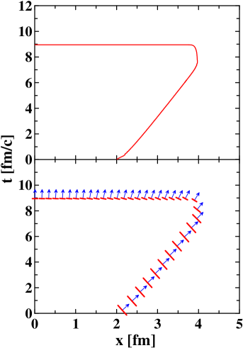
Figure 1: (Color online) Freeze-out hypersurface for hydrodynamic evolution the 1D step-like slab of nuclear matter. The upper panel displays the Cooper–Frye choice for the hypersurface. The lower panel schematically illustrates the modified Milekhin’s prescription, cf. Eq. (27), for the hypersurface. Arrows indicate local 4-velocities on this hypersurface. This figure is borrowed from Ref. 3FD-FO .

IV.3 Cooper–Frye Freeze-out

The Cooper–Frye hypersurface Cooper is constructed on the condition that this hypersurface is continuous, see Fig. 1 (upper panel). In the Cooper–Frye approach parameters of the distribution function, $\mu$, $T$ and $u^{\mu}$, are determined from Eqs. (4)–(6). The invariant spectrum of observable particles is expressed as follows

$$\left(E\frac{dN}{d^{3}p}\right)_{\mbox{\scriptsize Cooper--Frye}}=\Delta\sigma\ n_{\mu}p^{\mu}\ f(p,x),$$ (28)

where $n_{\mu}$ is the normal 4-vector to the $\Delta\sigma$ pieces of the continuous hypersurface. This formula cannot be already associated only with choice of a reference frame. It can be done, if $n_{\mu}n^{\mu}=1$, i.e. if $n^{\mu}$ is time-like. However, no frame corresponds to $n_{\mu}n^{\mu}=-1$. Parts of the hypersurface with space-like $n^{\mu}$ are unavoidable consequence of continuity of it. Precisely with these parts connected is a problem of the Cooper–Frye method. If $n_{\mu}p^{\mu}<0$, occurring at space-like $n^{\mu}$, the spectrum of Eq. (28) is negative Sinyukov89 ; Bugaev96 . This is a severe problem of the method. Note that above discussed recipes (20) and (27) do not reveal this problem.

An important option of the above constructions is weather the frozen-out matter is removed from the hydrodynamic evolution or not. This removal is associated with certain drain terms, $Q$ and $R^{\nu}$, in the r.h.s. of hydrodynamic equations

$$\partial_{\mu}J^{\mu}=Q,$$ (29)

$$\partial_{\mu}T^{\mu\nu}=R^{\nu},$$ (30)

where $J^{\mu}$ and $T^{\mu\nu}$ are the baryon current and energy-momentum tensor, respectively. An example of such drain terms is presented in Ref. 3FD-FO .

The Cooper–Frye method unambiguously implies that the freeze-out does not affect the hydrodynamic evolution of the system, i.e. the frozen-out matter is not removed from the hydrodynamic phase: $Q_{\mbox{\scriptsize CF}}=0$ and $R^{\nu}_{\mbox{\scriptsize CF}}=0$. The Cooper–Frye freeze-out, which is applied in the major part of hydrodynamic calculations now, proceeds in the following way. The hydro calculation runs absolutely unrestricted. The freeze-out hypersurface is determined by analyzing the resulting 4-dimensional field of hydrodynamic quantities on the condition of the freeze-out criterion being met.

At the same time, the modified Milekhin’s method (27) and the freeze-out in the computation frame (20) can be used in both regimes. In both cases the energy and momentum are conserved. Examples of the modified Milekhin’s method with and without removal of the frozen-out matter from the hydrodynamic evolution are presented in Ref. 3FD-FO . The removal of the matter indeed affects the system evolution. This influence is illustrated in Fig. 2. The freeze-out criterion used in this calculation stated that the matter is frozen-out when the local energy density $\varepsilon$ gets lower than 0.4 GeV/fm³. The $\varepsilon=0.4$ GeV/fm³ characteristic curves calculated with and without freeze-out turn out to be different. Note that the value $\varepsilon=0.4$ GeV/fm³ is achieved right at the surface of the system, if the frozen-out matter is removed. At the same time the $\varepsilon=0.7$ GeV/fm³ characteristic curves, which lie quite deep inside the system, remain fairly unaffected by the freeze-out.

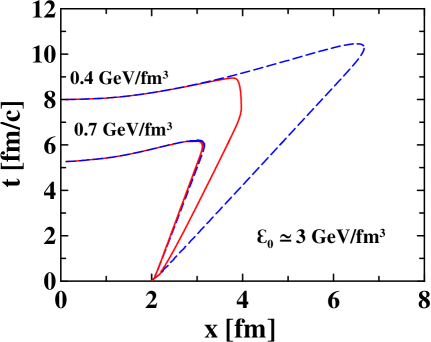
Figure 2: (Color online) Characteristic curves, corresponding to constant values of the energy density $\varepsilon$, for hydrodynamic evolution the 1D step-like slab of the 4 fm width. Initial conditions for this slab are constructed on the assumption that they are formed by the shock-wave mechanism in head-on collisions of two 1D slabs at $E_{\mbox{\scriptsize lab}}=$ 10 $A$ GeV. Thus constructed initial state corresponds to the initial energy density $\varepsilon_{0}\simeq$ 3 GeV/fm³. Characteristic curves correspond to $\varepsilon=0.4$ and 0.7 GeV/fm³, calculated with (solid lines) and without (dashed lines) removal of the frozen-out matter from the hydrodynamic evolution. This figure is borrowed from Ref. 3FD-FO .

V Discussion

We considered a puzzle which was in fact a prime motivation of the Cooper–Frye Cooper approach to the freeze-out in relativistic hydrodynamics. The puzzle consists in the fact that naive calculation of the total energy-momentum of unbound equilibrium system does not produce a 4-vector and, moreover, depends on the reference frame. We argue that a finite unbound system which is equilibrium in one reference frame is in general nonequilibrium in another frame. This is a consequence of the relative character of the time synchronization in the relativistic physics. Thus, naive assumption that this system is equilibrium in any reference frame results in this puzzle. Solution of the puzzle reveals that the Cooper–Frye recipe is far not a unique phenomenological method that meets requirements of energy-momentum conservation. Alternative freeze-out recipes are considered and discussed.

The above discussion concerned precisely phenomenological methods. Recently microscopic treatments of the freeze-out process were advanced based on the Bolzmann equation Sinyukov02 ; Sinyukov08 and Kadanoff–Baym equations Knoll08 . It was found that these microscopic approaches approximately justify Cooper–Frye formula (28) but only on the space-like part of the freeze-out hypersurface (i.e. possessing a time-like normal vector). Note that on this part of the hypersurface the Cooper–Frye method is very close to the modified Milekhin’s method (27) (cf. Fig. 1) as well as to the freeze-out in the computation frame (20). The Cooper–Frye formula on the time-like part of the freeze-out hypersurface is not reproduced by these treatments. Precisely on this part the Cooper–Frye formula essentially differs from two above mentioned alternative methods and also meets the problem of the negative spectrum.

Two main conclusions have been drawn from these microscopic considerations. First, the frozen-out matter should be removed from the hydrodynamic evolution. This removal is important for the total energy-momentum conservation. This conclusion testifies certainly not in favor of the standard Cooper–Frye method. Another basic conclusion is that sharp freeze-out at some 3D hypersurface is a rather rough approximation to the spectrum formation, because the freeze-out process is fairly extended in space and time. It means that the particle emission takes place from an extended 4-volume rather than from a 3-dimensional hyposurface as it is assumed in all above considered phenomenological methods. This conclusion is also supported by kinetic simulations, see e.g. Pratt08 . Therefore, it makes all above phenomenological methods questionable. However, the numeric implementation of the microscopic methods developed in Refs. Sinyukov02 ; Sinyukov08 ; Knoll08 in 3D hydrodynamic simulations is highly complicated, because it requires integration over future evolution of the system for the calculation of the particle emission at fixed time instant. The implementation performed in Refs. Sinyukov08 is not quite consistent, since it does not take into account the removal of the freeze-out with the hydrodynamic evolution. Therefore, we still have to use phenomenological methods of freeze-out in actual hydrodynamic simulations of heavy-ion collisions. The pending problem is to find out which of the phenomenological methods most closely simulates results of the microscopic methods.

References

- (1) R.B. Clare and D. Strottman, Phys. Rept. 141 177 (1986).
- (2) H. Stoecker and W. Greiner, Phys. Rept. 137, 277 (1986).
- (3) I.N. Mishustin, V.N. Russkikh, and L.M. Satarov, Yad. Fiz. 54, 429 (1991) [Sov. J. Nucl. Phys. 54, 260 (1991)].
- (4) D.H. Rischke, arXiv:nucl-th/9809044.
- (5) P.F. Kolb and U.W. Heinz, in ‘‘Quark Gluon Plasma 3’x’, Eds. R.C. Hwa and X.N. Wang (World Scientific, Singapore, 2004), [nucl-th/0305084].
- (6) P. Huovinen, P.V. Ruuskanen, Ann. Rev. Nucl. Part. Sci. 56, 163 (2006) [nucl-th/0605008].
- (7) G.A. Milekhin, Zh. Eksp. Teor. Fiz. 35, 1185 (1958); Sov. Phys. JETP 35, 829 (1959); Trudy FIAN 16, 51 (1961).
- (8) L.D. Landau, Izv. AN SSSR Nauk Ser. Fiz. 17, 51 (1953); S.Z. Belenkij, L.D. Landau, Nuovo Cim. Suppl. 3, 15 (1956), Usp. Fiz. Nauk 56, 309 (1955).
- (9) F. Cooper and G. Frye, Phys. Rev. D 10, 186 (1974).
- (10) S.T. Belyaev and G.I. Budker, Dokl. AN SSSR 107, 807 (1965).
- (11) Steven Weinberg, ‘‘Gravitation and Cosmology: Principles and Applications of the General Theory of Relativity’’ (John Wiley and Sons, New York, 1972), Chapter 2, sects. 6 and 8.
- (12) V.N. Russkikh and Yu.B. Ivanov, Phys. Rev. C 76, 054907 (2007) [nucl-th/0611094].
- (13) Yu.B. Ivanov, V.N. Russkikh, and V.D. Toneev, Phys. Rev. C 73, 044904 (2006) [nucl-th/0503088].
- (14) Yu.M. Sinyukov, Z. Phys. C43, 401 (1989).
- (15) K.A. Bugaev, Nucl. Phys. A606, 559 (1996).
- (16) Yu.M. Sinyukov, S.V. Akkelin, and Y. Hama, Phys. Rev. Lett. 89, 052301 (2002) [nucl-th/0201015].
- (17) S.V. Akkelin, Y. Hama, Iu.A. Karpenko, and Yu.M. Sinyukov, Phys. Rev. C 78, 034906 (2008) (arXiv:0804.4104 [nucl-th]).
- (18) J. Knoll, arXiv:0803.2343 [nucl-th].
- (19) S. Pratt and J. Vredevoogd, arXiv:0809.0516 [nucl-th].