A study of binary constraints for seismology of $\delta$ Scuti stars

Abstract

Seismology of single $\delta$ Scuti stars has mainly been inhibited by failing to detect many of the theoretically predicted pulsation modes, resulting in difficulties with mode identification. Theoretical and observational advances have, however, helped to overcome this problem, but the following questions then remain: do we know enough about the star to either use the (few) identified mode(s) to probe the structure of the star? or improve the determination of the stellar parameters? It is now generally accepted that for the observed frequencies to be used successfully as seismic probes for these objects, we need to concentrate on stars where we can constrain the number of free parameters in the problem, such as in binary systems or open clusters. The work presented here, investigates how much is gained in our understanding of the star, by comparing the information we obtain from a single star with that of an eclipsing binary system. Singular Value Decomposition is the technique used to explore the precision we expect in terms of stellar parameters (such as mass, age and chemical composition) as well as how these parameter uncertainties propagate to the Luminosity-Temperature (L-T) diagram. This work shows that the information content of the binary system provides sufficient constraints on the models so that the mode can be used to probe the star’s structure.

1 Introduction

$\delta$ Scuti stars are a class of pulsating stars located on the Hertzsprung-Russell Diagram on or around the Main Sequence and intersecting the instability strip. They are 1.5 - 2.5 $M_{\odot}$ stars pulsating often in one main dominant oscillation mode or many lower amplitude pulsation modes. They have been interesting targets seismologically, because the oscillation amplitudes often reach tenths of magnitudes, and we understand their stellar structure relatively well, so seismology can allow us to probe details of the microphysics such as energy transport mechanisms, convective core overshoot, as well as other less well-developed theories such as rapid rotation.

The main setbacks that $\delta$ Scuti seismology face (as well as other pulsating stars) are 1) the fundamental stellar parameters are not well-enough constrained to allow the few pulsation modes to probe the structure, and 2) rapid rotation causes each of the degrees $l$ to split into $2l+1$ $m$-modes, making mode-identification a difficult task [1]. Indeed these problems are not exclusive nor exhaustive. This has prompted authors to look towards objects where at least one of these problems can be eliminated [2, 3, 4, 5]. Observing stars where the number of free parameters is constrained, such as in open clusters or multiple systems is a possibility for overcoming these obstacles.

In order to use seismology to probe the interior of a star, the parameters of the star need to be known quite well, for example, the mass should be known to 1-2% [6]. The observables from a binary system provide strict constraints on the parameters of the component stars. If the binary is an eclipsing and spectroscopic system, the absolute values of the masses and radii can be extracted to 1-2% (e.g. [7, 8]).

The objective of this study is to find out if the uncertainties in the stellar parameters can be reduced, so that seismology can be applied to those stars that exhibit one or few pulsation modes. We look at the particular case of a pulsating star in an eclipsing binary system and compare the parameter uncertainties with those of an isolated star. This study quantifies how well the stellar parameters can be extracted in various hypothetical systems.

2 Methods

The mathematical basis of this study lies in the application of Singular Value Decomposition (SVD) techniques to physical models. This technique has been used in previous studies, such as [9, 10, 6] and it is being applied to many other areas of astrophysics and science, because of its powerful diagnostic properties. Intricate details of this mathematical technique are elaborated upon in the above mentioned publications as well as in [11]. Here we give the basic equations to enable an understanding of this work.

2.1 Singular Value Decomposition

SVD is the decomposition of any $M\times N$ matrix D into 3 components ${\bf U}$, ${\bf V^{T}}$ and ${\bf W}$ given by ${\bf D}={\bf UWV^{T}}$. ${\bf V^{T}}$ is the transpose of ${\bf V}$ which is an $N\times N$ orthogonal matrix that contains the input basis vectors for ${\bf D}$, or the vectors associated with the parameter space. ${\bf U}$ is an $M\times N$ orthogonal matrix that contains the output basis vectors for ${\bf D}$, or the vectors associated with the observable space. ${\bf W}$ is a diagonal matrix that contains the singular values of ${\bf D}$.

The key element to our work is the description of the matrix D. Here we define D to be a matrix whose elements consist of the partial derivatives of each of the observables with respect to each of the parameters of the system, in function of the expected measurement errors on each of the observables:

$$D_{ij}=\frac{\partial B_{i}}{\partial P_{j}}\epsilon_{i}^{-1}.$$ (1)

Here $B_{i}$ are each of the $i=1,2,...M$ observables of the system, with measurement or expected errors $\epsilon_{i}$, and $P_{j}$ are each of the $j=1,2,...,N$ free parameters of the system (see section 2.2 for discussion on the observables and the parameters).

By writing the design matrix in function of the measurement errors, we provide a quantitative description of the information content of each of the observables for determining the stellar parameters and their uncertainties.

Supposing that we are looking for the true solution ${\bf P}_{\rm R}$ of the system. By starting from an initial close guess of the solution ${\bf P}_{0}$, SVD can be used as an inversion technique by calculating a set of parameter corrections ${\bf\delta P}$ that minimizes some goodness-of-fit function: ${\bf\delta P=V\bar{W}^{-1}U^{T}\delta B}$, where ${\bf\delta B}$ are the differences between the set of actual observations O and the calculated observables ${\bf B}_{\rm 0}$ given the initial parameters ${\bf P}_{\rm 0}$. ${\bf\bar{W}}$ is a modification of the matrix W such that the inverse of the values below a certain threshold are set to 0. The formal errors are comprised of the sum of all of the ${\bf V}_{k}/w_{k}$, where each ${\bf V}_{k}/w_{k}$ describes the direction and magnitude to move each parameter, so that the true solution ${\bf P}_{\rm R}$ and formal uncertainties can be given by

$${\bf P}_{\rm R}={\bf P}_{\rm 0}+{\bf V\bar{W}^{-1}U^{T}\delta B}\left(\pm\frac{{\bf V}_{1}}{w_{1}}\pm\frac{{\bf V}_{2}}{w_{2}}\pm...\pm\frac{{\bf V}_{N}}{w_{N}}\right).$$ (2)

The covariance matrix C consequently comes in a very neat and compact form:

$$C_{jl}=\sum_{k=1}^{N}\frac{V_{jk}V_{lk}}{w_{k}^{2}},$$ (3)

and the square roots of the diagonal elements of the covariance matrix are the theoretical parameter uncertainties:

$$\sigma_{j}^{2}=\sum_{k=1}^{N}\left(\frac{V_{jk}}{w_{k}}\right)^{2}.$$ (4)

2.2 Observables, Parameters & Models

We describe a single $\delta$ Scuti star by a set of parameters or ingredients. The ingredients for the stellar model are mass $M$, age $\tau$, rotational velocity $v$, initial Hydrogen and heavy metals mass fraction $X$ and $Z$ where $X+Y+Z=1$ and $Y$ is initial Helium mass fraction, and mixing-length parameter $\alpha$ where applicable. The distance to the object $d$ is also included as a parameter.

For a binary system, the additional parameters are the system properties: separation of components $a$, eccentricity of orbit $e$, longitude of periastron $\omega$ and inclination of orbit $i$. Fortunately, both stellar components in a binary system share the parameters $\tau$, $X$ and $Z$, so then the individual stars differ mainly by $M$ and $v$. The parameters of the binary system of this study are given in Table 1.

The observables are the measurable quantities of the system. These include things such as radius, effective temperature, gravity, metallicity and parallax for a single star system. For a binary system, the observables include effective temperature ratio, relative radii, radial velocities and orbital period. The Aarhus STellar Evolution Code [12] is used to calculate the stellar evolution models. This code uses the stellar parameters as the input ingredients, and returns a set of global stellar properties such as radius and effective temperature, as well as the interior profiles of the star such as mass, density and pressure. Oscillation frequencies for this rapidly rotating star are calculated using MagRot [13, 14]. Using the global stellar properties and the distance to the star, SDSS [15] magnitudes and colours in various filters are evaluated using the Basel model atmospheres [16]. Most of the binary observables are calculated analytically using the combined stellar and binary parameters. In this work we refer to the non-seismic data as the classical observables. Most of the classical observables of the binary system are given in Table 1.

A clear distinction should be made between the input parameters of the system and output measurable quantities, the observables. So to discriminate between the errors in both parameters and observables, we shall denote the (derived) parameter uncertainties by $\sigma$, while $\epsilon$ is reserved for the observable errors.

Both luminosity and effective temperature can be observables, but in Section 3.2 the derived uncertainties of these properties are discussed. This refers specifically to the calculated error boxes in the luminosity-temperature (L-T) diagram, and here their uncertainties will also be denoted by $\sigma$.

Table 1: System Parameters & Observables

Parameter	Value ($P_{j}$)			Observable	Value ($O_{i}$)	$\epsilon_{i}$
$M_{A}$	1.8 $M_{\odot}$			$R_{A}$	1.95 $R_{\odot}$	0.02
$M_{B}$	1.7 $M_{\odot}$			$R_{B}$	1.81 $R_{\odot}$	0.02
$\tau$	0.7 Gyr			$T_{B}/T_{A}$	0.97	0.05
$X$	0.700			$T_{\rm eff}$	6965 (K)	100
$Z$	0.035			[M/H]	0.31 (dex)	0.05
$v_{A}$	100.0 km s-1			$v_{A}\sin i$	99.7 km s-1	2.5
$v_{B}$	80.0 km s-1			$v_{B}\sin i$	59.8 km s-1	2.5
$d$	200 pc			$\pi$	5.0 (mas)	0.5
$a$	0.15 AU			$\Pi$	0.031 (yrs)	0.00001
$i$	85.6 ∘			$i$	85.6 ∘	0.05
$e$	0.0			$M_{A}\sin^{3}i$	1.78 $M_{\odot}$	0.06
$\omega$	0.0			$M_{B}\sin^{3}i$	1.69 $M_{\odot}$	0.05

3 Results

The theoretical uncertainties in each of the parameters of $M_{A}$, $\tau$, $X$ and $Z$ are calculated as a function of error in radius $\epsilon_{R_{\star}}$ and as a function of error in colour $\epsilon_{(i-z)}$, using Equation 4 coupled with the observable errors given in Table 1. Consequently the theoretical uncertainties in luminosity and effective temperature are calculated using Equation 2, for three different values of $\epsilon_{R_{\star}}$ and three different values of effective temperature error $\epsilon_{T_{\rm eff}}$. The results are shown in Figures 1 and 2 below.

3.1 Parameter Uncertainties

Figure 1 shows the theoretical uncertainties ($\sigma$) in $M_{A}$, $\tau$, $X$ and $Z$ of a pulsating star as a function of error in the radius (left panels) and as a function of error in the photometric colours (right panels). Note that the left panels do not include photometric information, i.e. no colours nor magnitudes. The dashed lines show the results for a single star (the observables are radius, effective temperature, gravity, metallicity, …) while the solid lines show the results for a component of a binary system (observables are those of the single star and the binary observables). The lines with the diamonds include one identified mode as well as the classical observables. The results for the other stellar parameters are not shown, because the four aforementioned parameters and $v_{A}$ are responsible for determining the model structure of the pulsating star. $\sigma(v_{A})$ is is usually independent of $\epsilon_{R_{\star}}$ and $\epsilon_{(i-z)}$; it is determined mainly by the observables $v\sin i$ and $i$ from a combination of spectroscopy and the photometric light curve.

Figure 1: Theoretical uncertainties ($\sigma$) in mass $M$, age $\tau$, initial hydrogen $X$ and metal $Z$ content as a function of observable error. The left panel shows the uncertainties as a function of observable radius error, here no photometric information has been included. The right panel shows the uncertainties as a function of observable error in photometric colour. The dashed and continuous lines show the results for the single star and the binary system respectively, those with diamonds show the results when an identified mode is included in the set of observables.

For the single star without an identified mode (dashed lines no diamonds), the parameter uncertainties remain at a large constant value as a function of radius (left panels) but do decrease slightly with improved photometric data (right panels). Only when seismic data are included for the single star system (dashed lines, diamonds) and the observable errors are small, the parameters are constrained to a usable amount.

By comparing the solid lines with and without diamonds in Figure 1, it can be seen that the addition of one identified mode makes almost no difference to the parameter uncertainties for the binary system. This implies that there is enough information provided by the binary constraints to sufficiently determine the stellar parameters. In this sense, the identified mode is redundant information, and thus can be used maybe to test the interior of the star.

Including photometric information (right panels) provides an interesting result: the information provided by the single star system can supersede that of the binary system for $\tau$ and $Z$ . This is because the colours are uncontaminated by a component star. This only happens at very small measurement errors, and only when an identified mode is included for the single star.

3.2 Luminosity-Temperature Error Box

The correlation matrices come in a compact form when using SVD. This then allows a calculation of the theoretical uncertainties in both effective temperature and luminosity (L-T) (Equation 2). Figure 2 shows the theoretical error box in effective temperature and luminosity for a single star system (dashed lines) and a binary system (solid lines). The observables do not include photometric information, and for the single star an identified mode is included, while for the binary system no seismic data is included.

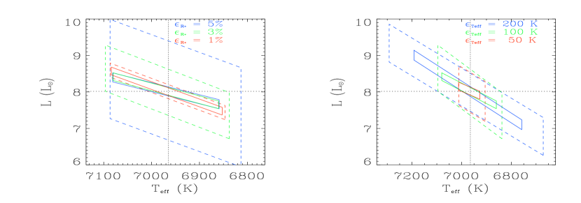
Figure 2: The theoretical error boxes for luminosity and effective temperature. The dashed lines represent the results for the single star while the continous lines represent the results for the binary system. The left panel shows the results while reducing the error in radius, and the right panel shows the results while reducing the error in effective temperature.

3.2.1 Single Star

Observe how the error box reduces significantly while reducing the error in the radius observable (left panel). The uncertainty in $T_{\rm eff}$ also reduces slightly. The right panel also shows that by reducing the errors in the observable $T_{\rm eff}$, an expected corresponding reduction in the uncertainties in $T_{\rm eff}$ is noted. The $\epsilon_{T_{\rm eff}}$ of 200, 100, and 50 K, produces a $\sigma(T_{\rm eff})$ of 250, 110, and 50 K. The fact that these uncertainties are reproduced also gives confidence in this method. $\sigma(L_{\star})$ changes slightly as a function of $\epsilon_{T_{\rm eff}}$, its value is determined mostly by the error in the radius observable (2%). Looking back to the left panel, we see that interpolating between 1% and 3% $\epsilon_{R_{\star}}$ produces a $\sigma(L_{\star})$ = 0.5 L_⊙ for $\epsilon_{R_{\star}}$ = 2%. This is the value that is shown in the right panel.

3.2.2 Binary System

For the binary system (solid lines), no identified mode is included. The error box for the binary system does not reduce while reducing the errors in the radius, because of the small uncertainties in these parameters. However, the error box does reduce when the error in effective temperature is reduced, reproducing accurately the input $\epsilon_{T_{\rm eff}}$ of $\sigma(T_{\rm eff})$ = 200, 100, and 50 K. $\sigma(L_{\star})$ does not decrease in either panel, because the mass is well-determined for the binary system and provides this narrow constraint on $L_{\star}$.

In all cases, note that the constraints provided by the binary system without an identified mode are more effective than those from the single star when an identified mode is included.

4 Conclusions

This study investigated whether the uncertainties in the stellar parameters of a pulsating component in an eclipsing binary system were sufficient so that an observed pulsation mode could be used to test the physics of the stellar interiors. Additionally we studied the information content of a pulsating star in a single star system to quantify how much is gained in terms of precision in parameters and size of the L-T error box by observing the star in a detached eclipsing binary system. The conclusions are summarized as follows:

• A single star system without an identified mode remains poorly understood when observables such as the radius or colours are poorly measured. The parameter uncertainties are too large to correctly place the star in the L-T diagram.

• A binary system without seismic information provides better constraints than the single star system when an oscillation mode has been identified.

• Reducing the size of some observable errors has little or no impact on the parameter determinations for the binary system, because these parameters are already well constrained.

• The tight constraints provided by the binary system for the stellar parameters reduces the size of the error box in the L-T diagram significantly.

• By carefully constraining the parameters of the star, just as an eclipsing binary system allows us to do, an accurate estimate of the stellar model under study can be obtained. This allows the redundant observables (like an oscillation mode) to be used exclusively to test the physics of the interior of a star.

References

References

- [1] Goupil, M.-J., Dupret, M. A., Samadi, R., Boehm, T., Alecian, E., Suarez, J. C., Lebreton, Y., & Catala, C. 2005, Journal of Astrophysics and Astronomy, 26, 249
- [2] Lampens, P., & Boffin, H. M. J. 2000, Delta Scuti and Related Stars, 210, 309
- [3] Aerts, C., & Harmanec, P. 2004, Spectroscopically and Spatially Resolving the Components of the Close Binary Stars, 318, 325
- [4] Maceroni, C. 2006, Astrophysics of Variable Stars, 349, 41
- [5] Costa et al., 2007, it A&A, 468, 637
- [6] Creevey, O.L., Monteiro, M.J.P.F.G., Brown, T.M., Metcalfe, T.M., Jiménez-Reyes, S.J., Belmonte, J.A., 2007, ApJ, 659, 616
- [7] Ribas, I., Jordi, C., & Torra, J. 1999, MnRAS, 309, 199
- [8] Lastennet, E., Valls-Gabaud, D., & Oblak, E. 2000, IAU Symposium, 200, 164P
- [9] Brown, T. M., Christensen-Dalsgaard, J., Weibel-Mihalas, B., & Gilliland, R. L. 1994a, ApJ, 427, 1013
- [10] Miglio, A., & Montalbán, J. 2005, A&A, 441, 615
- [11] Press, W. H. Teukolsky, S. A., Vetterling, W. T., Flannery, B. P., 1992, 2nd Ed., Cambridge University Press.
- [12] Christensen-Dalsgaard, J. 1982, MNRAS, 199, 735
- [13] Gough, D.O., Thompson, M.J, 1990, MNRAS, 242, 25
- [14] Burke, K.D., Thompson, M.J, 2006, ESASP, 624, 107
- [15] York, D. G., et al. 2000, it AJ, 120, 1579
- [16] Lejeune, T., Cuisinier, F., & Buser, R. 1997, A&AS, 125, 229