Quantum transport in honeycomb lattice ribbons with armchair and zigzag edges coupled to semi-infinite linear chain leads

Abstract

We study quantum transport in honeycomb lattice ribbons with either armchair or zigzag edges. The ribbons are coupled to semi-infinite linear chains serving as the input and output leads and we use a tight-binding Hamiltonian with nearest-neighbor hops. For narrow ribbons we find transmission gaps for both types of edges. The center of the gap is at the middle of the band in ribbons with armchair edges. This symmetry is due to a property satisfied by the matrices in the resulting linear problem. In ribbons with zigzag edges the gap center is displaced to the right of the middle of the band. We also find transmission oscillations and resonances within the transmitting region of the band for both types of edges. Extending the length of a ribbon does not affect the width of the transmission gap, as long as the ribbon’s length is longer than a critical value when the gap can form. Increasing the width of the ribbon, however, changes the width of the gap. In armchair edges the gap is not well-defined because of the appearance of transmission resonances while in zigzag edges the gap width systematically shrinks as the width of the ribbon is increased. We also find only evanescent waves within the gap and both evanescent and propagating waves in the transmitting regions.

1 Introduction

Graphene is a single layer of carbon atoms in a honeycomb lattice and serves as the basic building block of fullerenes like carbon nanotubes saito98 . It has recently been found to be stable under ambient conditions novoselov04 ; novoselov05 and has unique charge carrier properties novoselov05b ; zhang05 ; geim07 . Graphene nanoribbons are quasi-one-dimensional honeycomb lattice sheets with finite widths. Because of the width termination charge carriers become confined and the appearance of an energy gap is expected son06 ; fujita96 ; nakada96 ; wakabayashi99 ; ezawa06 ; brey06 ; sasaki06 ; abanin06 ; barone06 . For a recent review see reference castro09 . Graphene nanoribbons have been fabricated using lithography han07 , lithography and etching chen07 , epitaxial growth and lithography berger06 , chemical growth li08 , and deposition and etching ozyilmaz07 techniques. Measurements on these nanoribbons found a conductance gap that scales inversely with the width of the ribbons han07 ; ozyilmaz07 .

Possible edge types of regular graphene nanoribbons can be armchair or zigzag edges, on both sides of the ribbon. Theoretical studies using tight-binding band calculations based on the $\pi$-states of carbon fujita96 ; nakada96 ; wakabayashi99 ; ezawa06 and studies on the solution of the two-dimensional free massless Dirac equation using specific boundary conditions brey06 ; sasaki06 ; abanin06 found different transport properties for ribbons with armchair edges than those with zigzag edges. Ribbons with armchair edges can be either metallic or semiconducting depending on the width of the ribbon while ribbons with zigzag edges are metallic. Furthermore, the existence of special edge states localized at the zigzag edges gives rise to flat bands at the Fermi level in ribbons with zigzag edges. On the other hand, ab initio calculations on graphene nanoribbons with hydrogen passivated edges found band gaps in both armchair and zigzag edges son06 . Another density functional theory calculation, however, found that hydrogen termination can affect the properties of the ribbon barone06 .

In molecular electronics the search for conducting molecular wires that can be used in the construction of devices such as field effect transistors has been actively pursued. Wires made of linked thiophene units otsubo01 ; robertson03 ; pearman03 ; bong04 and alternating thiophene and ethynyl units tam06 have been synthesized with lengths up to $11$ nm. The synthesis of a chain of copper ions surrounded by helical ligand strands has also recently been reported schultz08 . Such molecular wires can be coupled to electrodes such as cut nanotubes guo06a ; guo06b or gold break junctions venkataraman06 ; park07 .

In this paper we study quantum transport in honeycomb lattice ribbons using a tight-binding model with nearest-neighbor hops. The ribbons have either armchair or zigzag edges. In contrast to previous theoretical and numerical studies, however, we couple the ribbons to semi-infinite linear chains that serve as the input and output leads. Such a system may be realized experimentally as a nanoribbon of graphene in contact with molecular wires serving as the leads. We vary both the length and the width of the ribbons. For a chain of hexagons with either armchair or zigzag edges and coupled to input and output leads we find the existence of a transmission gap, as long as the ribbon is longer than a critical length below which the gap does not form. The center of this gap coincides with the middle of the band in ribbons with armchair edges but not with zigzag edges. This symmetry arises from a property of the matrices in the resulting linear problem. Extending the length of the ribbon does not affect the width of the transmission gap. Extending the width of the ribbon, however, affects the width of the gap. In ribbons with armchair edges the appearance of transmission resonances obscures the exact width of the gap while in ribbons with zigzag edges the gap systematically shrinks as the width of the ribbon is extended.

2 The model

We model the transport of a quantum particle using the tight-binding Hamiltonian

$$\mathcal{H}=\sum_{i=1}^{N_{s}}\epsilon_{i}\left|\varphi_{i}\right>\left<\varphi_{i}\right|+\sum_{<ij>}v_{ij}\Bigl{\{}\left|\varphi_{i}\right>\left<\varphi_{j}\right|+\left|\varphi_{j}\right>\left<\varphi_{i}\right|\Bigr{\}},$$ (1)

where the $\left|\varphi_{i}\right>$’s are tight-binding basis functions centered on site $i$, $N_{s}$ is the total number of lattice sites available for the particle to hop into, and the sum in the second term is only over nearest-neighbor sites. Randomly varying the on-site energies $\epsilon_{i}$ identifies the model as the Anderson model of localization anderson58 . Alternatively, setting the $\epsilon_{i}$ to a constant, choosing $v_{ij}$ to be a non-zero constant only for nearest neighbor sites, and embedding the transport in a disordered site-percolation cluster identifies the model as the quantum percolation model degennes59 ; kirkpatrick72 . Both the Anderson model and quantum percolation involve disorder. In this paper we follow the quantum percolation model, i.e., we set $\epsilon_{i}\!=\!0$ and let $v_{ij}$ be a non-zero constant only for nearest neighbor sites. The model, however, does not involve disorder. Particle transport is through perfectly ordered honeycomb lattice ribbons.

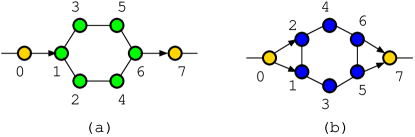
Figure 1: (color online) Hexagons in (a) armchair and (b) zigzag orientations. Semi-infinite input and output linear chains are connected to the hexagons. Beside each site is its label. Sites labelled $0$ and $N_{\rm r}\!+\!1$ are the input and output supersites, respectively. $N_{\rm r}$ is the number of sites within the hexagon.

Shown in Fig. 1 are hexagons oriented so that they form either armchair or zigzag edges in a honeycomb lattice ribbon. In a ribbon containing $N_{\rm r}$ sites, the site with label $0$ in the input chain and label $N_{\rm r}\!+\!1$ in the output chain are the only sites that are directly connected to the ribbon. We call these sites the input and output supersites, respectively. The connections between these supersites and the ribbon can be single-channel as shown in Fig. 1(a) or multi-channel as shown in Fig. 1(b). The distance between nearest-neighbor sites is set to $a_{0}\!=\!1$, thus setting the length scale of the model (although the length scale is actually inconsequential since $\mathcal{H}$ has no explicit length dependence).

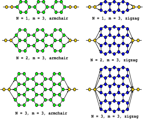
Figure 2: (color online) Honeycomb lattice ribbons of various widths. $N$ is the width label of a ribbon and $m$ is the number of hexagons in one hexagonal chain. Connections between the ribbon and the linear chain leads are also shown.

Shown in Fig. 2 are honeycomb lattice ribbons with either armchair or zigzag edges and with varying widths. The $N\!=\!1$ ribbon is a chain of hexagons coupled to the input and output leads. $m$ counts the number of hexagons in one hexagonal chain. The $N\!=\!2$ ribbon consists of two $N\!=\!1$ ribbons placed side by side. $N$ thus directly determines the ribbon width while $m$ determines the ribbon length.

We have used semi-infinite linear chains as the input and output leads to mimic linear molecular wires. Because of this linearity, an incident particle having a specific energy can have only one mode of either a propagating or evanescent wave bagwell90 impinging on the ribbon. We thus determine the effects of small honeycomb lattice ribbons of varying widths and lengths on the transmission of such single-mode waves. Recent studies have been done modelling the leads as normal metals having an aggregate number of modes incident on large honeycomb lattice ribbons schomerus07 ; blanter07 ; robinson07 . The leads were modelled as either square or honeycomb lattices. It was found that for sufficiently large ribbons the geometrical details of the leads were not critical schomerus07 . At the Dirac point of the ribbon evanescent waves are dominant while away from this point propagating waves dominate the transport blanter07 . In this study, in contrast, we deal with leads having only one mode incident on a small honeycomb lattice ribbon and see that the transmission of this incident wave depends strongly on the width, length, and edge type of the ribbon.

To determine the hopping transport properties of particles through honeycomb lattice ribbons the Hamiltonian in Eq. (1) is cast in a matrix representation with the $\left|\varphi_{i}\right>$’s as the basis. We write the eigenvector as $\vec{\psi}$, which is a column vector with elements $\varphi_{i}$ as the coefficients of the chosen basis. Because the linear chain leads are infinite the equivalent matrix problem is infinite-dimensional. The contribution of the leads (except for the supersites), however, can be factored out since each site in the chain only interacts with its nearest-neighbor sites to the left and right, thereby resulting in predictable tridiagonal elements in the Hamiltonian matrix. We follow the method proposed by Daboul et al. daboul00 by using the scattering boundary condition ansatz

$$\varphi_{n}=\left\{\begin{array}[]{ll}e^{inq}+r\>e^{-inq},&~{}~{}{\rm left~{}input~{}lead},\\ t\>e^{i(n-N_{r}-1)q},&~{}~{}{\rm right~{}output~{}lead},\\ \end{array}\right.$$ (2)

where $r$ and $t$ are the reflection and transmission amplitudes, respectively. Note that along the left input lead $n\!\leq\!0$ while along the right output lead $n\!>\!N_{r}$. The ansatz states that an incoming plane wave and a reflected wave with amplitude $r$ are in the input lead and a transmitted wave with amplitude $t$ is in the output lead. An alternative but equivalent approach is to use the non-equilibrium Green’s function technique to determine the transmission wang08 .

In general the hopping amplitudes along the left and right leads and the ribbon can be different. In this paper we consider the left and right leads to be the same and thus, the leads have the same hopping amplitudes $v_{\rm left}=v_{\rm right}=v_{\rm lead}$. Let $v$ be the hopping amplitude within the ribbon.

Using the ansatz we can reduce the original infinite-dimensional problem into a finite one. Along both leads we get the dispersion relation

$$e^{iq}+e^{-iq}=\frac{E}{v_{\rm lead}}.$$ (3)

Choosing a numerical value for $E$ and $v_{\rm lead}$ sets the value of $q$. Also, because of Eq. 3, the value of $E/v_{\rm lead}$ is bounded within the interval $\left[-2,2\right]$. For the ribbon, the problem reduces to a finite linear problem of the form $\mathsf{A}\vec{\psi}=\vec{b}$. In the armchair hexagon shown in Fig. 1(a), for example, we get

$$\mathsf{A}=\left(\begin{array}[]{cccccccc}-\alpha\!+\!i\beta&v_{\rm lead}&0&0&0&0&0&0\\ v_{\rm lead}&-E&v&v&0&0&0&0\\ 0&v&-E&0&v&0&0&0\\ 0&v&0&-E&0&v&0&0\\ 0&0&v&0&-E&0&v&0\\ 0&0&0&v&0&-E&v&0\\ 0&0&0&0&v&v&-E&v_{\rm lead}\\ 0&0&0&0&0&0&v_{\rm lead}&-\alpha\!+\!i\beta\\ \end{array}\right),$$

$$\vec{\psi}=\left(\begin{array}[]{c}1\!+\!r\\ \varphi_{1}\\ \varphi_{2}\\ \varphi_{3}\\ \varphi_{4}\\ \varphi_{5}\\ \varphi_{6}\\ t\\ \end{array}\right),\ {\rm and}\ \vec{b}=\left(\begin{array}[]{c}2i\beta\\ 0\\ 0\\ 0\\ 0\\ 0\\ 0\\ 0\\ \end{array}\right),$$ (4)

where $\alpha\!=\!E/2$, $\beta\!=\!\sqrt{4v^{2}_{\rm lead}\!-\!E^{2}}/2$.

We can determine $\vec{\psi}$ exactly by carefully taking the inverse of $\mathsf{A}$ and then multiplying it to $\vec{b}$. To do this we numerically decompose $\mathsf{A}$ using singular-value decomposition so that $\mathsf{A}=\mathsf{U}\>\mathsf{\Sigma}\>\mathsf{V}^{\rm\dagger}$, where $\mathsf{U}$ and $\mathsf{V}$ are unitary matrices and $\mathsf{\Sigma}$ is a diagonal matrix golub96 . The inverse can then be determined using the properties of unitary and diagonal matrices. Once we determine $\vec{\psi}$ we can then calculate the transmission coefficient by $T\!=\!\left|t\right|^{2}$. This numerically exact approach has also been employed in the study of localization in disordered clusters in two-dimensional quantum percolation cuansing08 ; islam08 .

The connections between the input and output supersites and the ribbon are reflected in the outermost rows and columns of $\mathsf{A}$. The inner rows and columns reflect the connections between sites within the ribbon. And so for the zigzag hexagon shown in Fig. 1(b) the corresponding matrix $\mathsf{A}$ will have almost the same central entries as that shown in Eq. (4) except for the extra entries along the outer rows and columns because of the additional channels available between the supersites and the hexagon.

A merit of determining all elements of $\psi$ exactly is that the components $\varphi_{i}$ of the wave function at all of the sites in the ribbon are also determined. In Sec. 3 we show plots of the wave function density in $N\!=\!1$, $m\!=\!8$ ribbons with armchair or zigzag edges.

3 Numerical results

Depending on the atomic composition of the ribbon and the leads, $v$ and $v_{\rm lead}$ are in general not the same. In our simulations, however, we set the values of $v$ and $v_{\rm lead}$ to one. We vary the energy from $E\!=\!-2$ to $E\!=\!2$ in energy steps of $\Delta E\!=\!0.01$. For each value of $E$ the complex-valued matrix $\mathsf{A}$ is constructed by noting the connections between the sites, including the supersites. The function $\vec{\psi}$ is then numerically determined via the singular-value decomposition of $\mathsf{A}$. The transmission coefficient $T$ is then calculated from $\left|t\right|^{2}$.

Shown in Fig. 3 are plots of the transmission coefficient $T$ as a function of the energy $E$ of the particle in $N\!=\!1$ ribbons. Ribbons with armchair edges are shown in Fig. 3(a) while those with zigzag edges are shown in Fig. 3(b). The length of the ribbons are $m\!=\!2$ and $m\!=\!8$ hexagons. For the ribbons with armchair edges we see symmetry between the positive and negative energy regions, i.e., with respect to the middle of the band. This symmetry in the sign of the energy arises from a condition satisfied by the $\mathsf{A}$ matrix for the ribbon with armchair edges and is discussed in Sec. 4. We also see two features as the length of the ribbons are increased from $m\!=\!2$ (red dots) to $m\!=\!8$ (black dots): (a) the number of transmission oscillations increases proportionally, and (b) a transmission gap develops. The transmission oscillations are reminiscent of the transmission resonances found in the square lattice case cuansing04 . The transmission gap develops as the length of the ribbon is extended. Although $T$ has a non-zero minimum at the middle of the band for $m\!=\!2$, this minimum falls to zero transmission for the first time when $m\!=\!6$. Extending the ribbon length further to $m\!=\!100$ increases the number of transmission oscillations and sharpens, but does not change the width, of the gap.

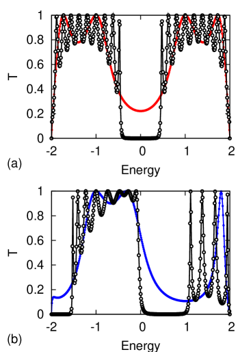
Figure 3: (color online) Transmission coefficient $T$ as a function of the particle’s energy in honeycomb lattice ribbons of width $N\!=\!1$. (a) Armchair edges with $m\!=\!2$ for filled (red online) circles and $m\!=\!8$ for open circles. The lines drawn are not analytical fits but simply connect adjacent datapoints to aid the eye. (b) Zigzag edges with $m\!=\!2$ for filled (blue online) circles and $m\!=\!8$ for open circles.

For the ribbons with zigzag edges we see in Fig. 3(b) that the number of transmission oscillations grows and a transmission gap develops as the length of the ribbon is extended from $m\!=\!2$ (blue dots) to $m\!=\!8$ (black dots), similar to the case for armchair edges. However, the center of the transmission gap is not at the middle of the band, which is now slightly transmitting. And in contrast to the armchair edges case, the number of oscillations in the $E\!>\!0$ region is half those in the $E\!<\!0$ region. The absence of symmetry with respect to the middle of the band in the transmission for ribbons with zigzag edges can be attributed to the extra connections between the input and output supersites and the ribbon, as discussed in Sec. 4.

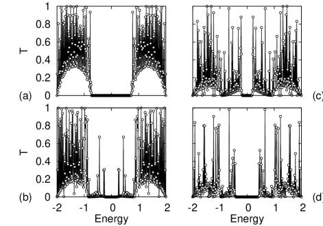
Figure 4: Transmission coefficient $T$ as a function of the particle’s energy $E$ in honeycomb lattice ribbons with armchair edges. The ribbons have length $m\!=\!100$. The widths are (a) $N\!=\!2$, (b) $N\!=\!3$, (c) $N\!=\!4$, and (d) $N\!=\!5$. The transmission gap is symmetric with respect to the middle of the band.

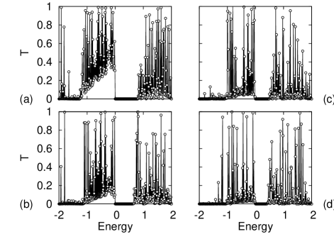
Figure 5: Transmission coefficient $T$ as a function of the particle’s energy $E$ in honeycomb lattice ribbons with zigzag edges. The ribbons have length $m\!=\!100$. The widths are (a) $N\!=\!2$, (b) $N\!=\!3$, (c) $N\!=\!4$, and (d) $N\!=\!5$. The transmission gap shrinks systematically as the ribbon’s width is increased.

Shown in Figs. 4 and 5 are plots on how the transmission coefficient behaves as a function of the energy of the particle as the width of the ribbons is varied from $N\!=\!2$ to $N\!=\!5$. The ribbons have length $m\!=\!100$ and have armchair edges in Fig. 4 and zigzag edges in Fig. 5. For the ribbons with armchair edges the transmission gap is symmetric with respect to the middle of the band. In contrast, for the ribbons with zigzag edges the center of the transmisison gap does not coincide with the middle of the band. In addition, the width of the gap decreases systematically as the width of the ribbon with zigzag edges is increased. This is not the case for the ribbons with armchair edges. Taking a closer look at Fig. 4(b) we see that transmission resonances appear in the region where there is a gap in the narrower ribbon shown in Fig. 4(a). As the ribbon’s width is increased transmission resonances appear within the gap and thus obscures the determination of the exact width of the gap.

We thus see in narrow ribbons with either armchair or zigzag edges a transmission gap dividing the transmission curve into two regions. As the width of the ribbon is increased the gap in ribbons with armchair edges is obscured by the appearance of transmission resonances within it while the gap in ribbons with zigzag edges systematically shrinks.

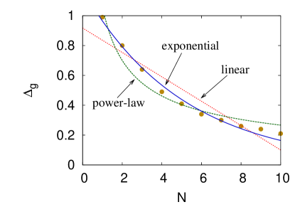
Figure 6: (color online) Transmission gap, $\Delta_{g}$, as a function of the width $N$ for $m\!=\!100$ ribbons with zigzag edges. Linear (red), power-law (green) and exponential (blue) fitting curves are also shown.

The dependence of the transmission gap, $\Delta_{g}$, on the width of the ribbon with zigzag edges can be determined. For ribbons with armchair edges, in contrast, the gap is not well-defined because of the appearance of resonances and thus there is no clear indication of the gap’s width. Shown in Fig. 6 is a plot of $\Delta_{g}$ as a function of $N$ for ribbons with zigzag edges. The length of the ribbons are $m\!=\!100$. Also shown are the curves for linear, power-law and exponential fits. The values of the fitting parameters are shown in Table 1. The correlation coefficients found for the three fits are close, with the exponential fit having the best value.

Table 1: Values of the fitting parameters found for the data shown in Fig. 6 for ribbons with zigzag edges.

linear fit:

$\Delta_{g}=(-0.082\pm 0.010)\>N+(0.917\pm 0.065)$, $\left|R\right|^{2}=0.928$

power-law fit:

$\Delta_{g}=(1.061\pm 0.058)\>N^{(-0.600\pm 0.049)}$, $\left|R\right|^{2}=0.967$

exponential fit:

$\Delta_{g}=(1.175\pm 0.038)\>e^{(-0.197\pm 0.009)\>N}$, $\left|R\right|^{2}=0.992$

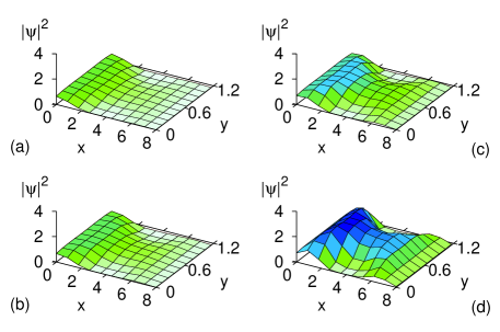
Figure 7: (color online) Wave function density in $N\!=\!1$, $m\!=\!8$ ribbons with zigzag edges. The energies are (a) $E\!=\!1.03$, (b) $E\!=\!1.05$, (c) $E\!=\!1.07$, and (d) $E\!=\!1.09$. These energies are in the region around the right edge of the transmission gap. The colors aid the eye in determining the height of $\left|\vec{\psi}\right|^{2}$.

Shown in Fig. 7 is the evolution of the wavefunction density $\left|\vec{\psi}\right|^{2}$ as the energy $E$ is varied from within the transmission gap into the $E\!>\!0$ transmitting region of the $N\!=\!1$, $m\!=\!8$ ribbon with zigzag edges. In the figure, the ribbon is along the $xy$-plane. The input lead is coupled to the ribbon at $x\!=\!0$ and the output lead is coupled at the other side. For energies within the transmission gap the wave function is zero. For energies near the edge of the gap, for example at $E\!=\!1.03$ as shown in Fig. 7(a), the wave function is almost zero everywhere except for a slight hump at the input side of the ribbon. This hump grows as the energy is increased until within the transmitting region a well-developed wave with a relatively large amplitude appears. Within the gap the wave is evanescent bagwell90 and trying to penetrate the ribbon. As we increase the energy of the particle the wave eventually gains enough energy to proceed into the ribbon and transmit to the other side.

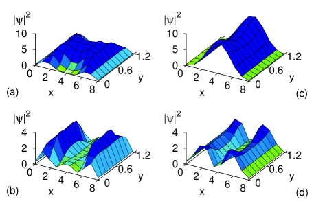
Figure 8: (color online) The $\left|\vec{\psi}\right|^{2}$ in $N\!=\!1$, $m\!=\!8$ ribbons with zigzag edges. These waves correspond to transmission peaks with energy values (a) $E\!=\!1.12$, (b) $E\!=\!1.38$, (c) $E\!=\!-1.52$, and (d) $E\!=\!-1.42$.

Shown in Fig. 8 are some of the wave function densities that correspond to transmission peaks in $N\!=\!1$, $m\!=\!8$ ribbons with zigzag edges. The wave in Fig. 8(a) is the highly transmitting wave that the waves in Fig. 7 develop into as the particle’s energy is increased. Compared to the waves in Fig. 7 the highly transmitting wave in Fig. 8(a) is sitting symmetrically at the center of the ribbon. This characteristic is a property satisfied by the wave functions that correspond to the transmission peaks in Fig. 3, including those for the armchair edges.

4 Symmetry of ribbons with armchair edges

In Fig. 3 the transmission coefficient for ribbons with armchair edges is shown to be symmetric with respect to a change in the sign of the energy. This symmetry arises from a property of the $\mathsf{A}$ matrix for the ribbon.

Consider, for example, the linear problem $\mathsf{A}\vec{\psi}\!=\!\vec{b}$ shown in Eq. (4) for the armchair hexagon. For a ribbon of $N_{r}$ sites the corresponding matrix $\mathsf{A}$ has size $\left(N_{r}\!+\!2\right)\times\left(N_{r}\!+\!2\right)$ and $\vec{\psi}$ and $\vec{b}$ are column vectors of size $\left(N_{r}\!+\!2\right)$. Suppose we have two linear problems, $\mathsf{A}\vec{\psi}_{1}=\vec{b}$ and $\mathsf{B}\vec{\psi}_{2}=\vec{b}$, with the same right-hand side $\vec{b}$. The $\vec{\psi}_{1}$ and $\vec{\psi}_{2}$ can be determined using the inverses of $\mathsf{A}$ and $\mathsf{B}$, i.e., $\vec{\psi}_{1}=\mathsf{A}^{-1}\vec{b}$ and $\vec{\psi}_{2}=\mathsf{B}^{-1}\vec{b}$. We can write the inverses of the matrices in terms of their corresponding matrix of cofactors,

$$\mathsf{A}=\frac{\mathsf{C}^{\rm{T}}}{\left|\mathsf{A}\right|},\ \rm{and}\ \mathsf{B}=\frac{\mathsf{D}^{\rm{T}}}{\left|\mathsf{B}\right|},$$ (5)

where $\left|\mathsf{A}\right|$ and $\left|\mathsf{B}\right|$ are the determinants of the matrices. Since $\mathsf{A}$ and $\mathsf{B}$ are symmetric, $\mathsf{C}^{\rm{T}}=\mathsf{C}$ and $\mathsf{D}^{\rm{T}}=\mathsf{D}$. In particular, $\vec{\psi}_{1}$ can be calculated from

$$\left(\begin{array}[]{c}1\!+\!r_{1}\\ \varphi_{1}\\ \vdots\\ \varphi_{N}\\ t_{1}\end{array}\right)=\frac{1}{\left|\mathsf{A}\right|}\left(\begin{array}[]{ccc}C_{0,0}&\cdots&C_{0,N_{r}\!+\!1}\\ C_{1,0}&\cdots&C_{1,N_{r}\!+\!1}\\ \vdots&\ddots&\vdots\\ C_{N_{r},0}&\cdots&C_{N_{r},N_{r}}\\ C_{N_{r}\!+\!1,0}&\cdots&C_{N_{r}\!+\!1,N_{r}\!+\!1}\\ \end{array}\right)\left(\begin{array}[]{c}2i\beta\\ 0\\ \vdots\\ 0\\ 0\\ \end{array}\right).$$ (6)

The transmission amplitude $t_{1}$ can be determined from the multiplication of the last row of $\mathsf{C}$ with $\vec{b}$. We get

$$t_{1}=\frac{2\,i\,\beta\,C_{N_{r}\!+\!1,0}}{\left|\mathsf{A}\right|}.$$ (7)

A similar calculation can be done to determine $t_{2}$. The transmission coefficients can then be calculated from $T_{1}=\left|t_{1}\right|^{2}$ and $T_{2}=\left|t_{2}\right|^{2}$.

Suppose $\mathsf{A}\!=\!\mathsf{A}(E)$ and $\mathsf{B}\!=\!\mathsf{A}(-E)$. The condition that a change in the sign of $E$ results in the same transmission coefficient, using Eq. (7), is

$$\left|C(E)_{N_{r}\!+\!1,0}\right|^{2}=\left|C(-E)_{N_{r}\!+\!1,0}\right|^{2},$$ (8)

where we use the fact that $\left|\mathsf{A}(E)\right|^{2}=\left|\mathsf{A}(-E)\right|^{2}$. For there to be symmetry between the positive and negative energy regions, Eq. (8) must be satisfied. Note that this condition is independent of the size of the ribbon, as long as that ribbon is coupled to input and output leads.

Calculating the cofactor $C(E)_{7,0}$ of $\mathsf{A}$ in Eq. (4), noting that in our simulations $v_{l}=v$, results in

$$\left|C(E)_{7,0}\right|^{2}=4v^{10}\left(E^{4}-2v^{2}E^{2}+v^{4}\right).$$ (9)

This is an even function of $E$ and thus satisfies the symmetry condition of Eq. (8). In contrast, for the zigzag hexagon its corresponding $\mathsf{A}$ matrix will have four more $v$ entries than the one shown in Eq. (4). This reflects the second channel available in the coupling between the supersites and the hexagon. The cofactor of the resulting $\mathsf{A}$ for this case leads to

$$\begin{array}[]{rcr}\left|C(E)_{7,0}\right|^{2}&=&4v^{8}(E^{6}+4vE^{5}+2v^{2}E^{4}-8v^{3}E^{3}\\ &&-7v^{4}E^{2}+4v^{5}E+4v^{6}).\\ \end{array}$$ (10)

Terms with odd powers of $E$ appear and the cofactor therefore will be different when the sign of $E$ is reversed. The symmetry condition in Eq. (8) is not satisfied and, as can be seen in Fig. 3(b), the profile of the transmission coefficient is different between the positive and negative energy regions. This analysis can be extended to ribbons with any $N$ and $m$. As can be seen in Figs. 4 and 5 the symmetry is preserved only in ribbons with armchair edges.

5 Summary

We investigate the transport of a quantum particle traversing through honeycomb lattice ribbons with either armchair or zigzag edges with varying length and width. The ribbons are coupled to semi-infinite linear chains that serve as the input and output leads. We have seen the role of coupling the leads to the ribbons. In narrow, $N\!=\!1$, ribbons we find transmission gaps for both types of edges. In armchair edges the center of the gap coincides with the middle of the band. This symmetry is due to a property of the corresponding $\mathcal{A}$ matrices. In zigzag edges the gap center is displaced to the positive energy region. We also find transmission resonances for both types of edges. These transmission resonances occur whenever the wave fits symmetrically within the ribbon, reminiscent of resonant tunneling but without having finite potentials or tunneling in this model. Increasing the length of the ribbons increases the number of transmission resonances without affecting the width of the transmission gap, as long as the ribbon is longer than a critical length when the gap can form. Increasing the width of the ribbons affects the width of the transmission gap. In ribbons with armchair edges transmission resonances appear within the gap as the ribbon width is extended. In ribbons with zigzag edges the gap systematically shrinks as the ribbon width is increased.

- (1) R. Saito, G. Dresselhaus, M.S. Dresselhaus, Physical Properties of Carbon Nanotubes (Imperial College Press, London, 1998)
- (2) K.S. Novoselov, A.K. Geim, S.V. Morozov, D. Jiang, Y. Zhang, S.V. Dubonos, I.V. Grigorieva, A.A. Firsov, Science 306, 666 (2004)
- (3) K.S. Novoselov, D. Jiang, F. Schedin, T.J. Booth, V.V. Khotkevich, S.V. Morozov, A.K. Geim, P. Natl. Acad. Sci. USA 102, 10451 (2005)
- (4) K.S. Novoselov, A.K. Geim, S.V. Morozov, D. Jiang, M.I. Katsnelson, I.V. Grigorieva, S.V. Dubonos, A.A. Firsov, Nature (London) 438, 197 (2005)
- (5) Y. Zhang, Y.W. Tan, H.L. Stormer, P. Kim, Nature (London) 438, 201 (2005)
- (6) A.K. Geim, K.S. Novoselov, Nature Materials 6, 183 (2007)
- (7) Y.W. Son, M.L. Cohen, S.G. Louie, Phys. Rev. Lett. 97, 216803 (2006)
- (8) M. Fujita, K. Wakabayashi, K. Nakada, K. Kusakabe, J. Phys. Soc. Jpn. 65, 1920 (1996)
- (9) K. Nakada, M. Fujita, G. Dresselhaus, M.S. Dresselhaus, Phys. Rev. B 54, 17954 (1996)
- (10) K. Wakabayashi, M. Fujita, H. Ajiki, M. Sigrist, Phys. Rev. B 59, 8271 (1999)
- (11) M. Ezawa, Phys. Rev. B 73, 045432 (2006)
- (12) L. Brey, H.A. Fertig, Phys. Rev. B 73, 235411 (2006)
- (13) K.I. Sasaki, S. Murakami, R. Saito, J. Phys. Soc. Jpn. 75, 074713 (2006)
- (14) D.A. Abanin, P.A. Lee, L.S. Levitov, Phys. Rev. Lett. 96, 176803 (2006)
- (15) V. Barone, O. Hod, G.E. Scuseria, Nano Lett. 6, 2748 (2006)
- (16) A.H. Castro Neto, F. Guinea, N.M.R. Peres, K.S. Novoselov, A.K. Geim, Rev. Mod. Phys. 81, 109 (2009)
- (17) M.Y. Han, B. Özyilmaz, Y. Zhang, P. Kim, Phys. Rev. Lett. 98, 206805 (2007)
- (18) Z. Chen, Y.M. Lin, M.J. Rooks, P. Avouris, Physica E 40, 228 (2007)
- (19) C. Berger, Z. Song, X. Li, X. Wu, N. Brown, C. Naud, D. Mayou, T. Li, J. Hass, A. Marchenkov et al., Science 312, 1191 (2006)
- (20) X. Li, X. Wang, L. Zhang, S. Lee, H. Dai, Science 319, 1229 (2008)
- (21) B. Özyilmaz, P. Jarillo-Herrero, D. Efetov, P. Kim, Appl. Phys. Lett 91, 192107 (2007)
- (22) T. Otsubo, Y. Aso, K. Takimiya, Bull. Chem. Soc. Japan 74, 1789 (2001)
- (23) N. Robertson, C.A. McGowan, Chem. Soc. Rev. 32, 96 (2003)
- (24) R. Pearman, D. Bong, R. Breslow, G.W. Flynn, Polym. Mater. Sci. Eng. 89, 213 (2003)
- (25) D. Bong, I.W. Tam, R. Breslow, J. Am. Chem. Soc. 126, 11796 (2004)
- (26) I.W. Tam, J. Yan, R. Breslow, Org. Lett. 8, 183 (2006)
- (27) D. Schultz, F. Biaso, A.R.M. Shahi, M. Geoffroy, K. Rissanen, L. Gagliardi, C.J. Cramer, J.R. Nitschke, Chem. Eur. J. 14, 7180 (2008)
- (28) X. Guo, J.P. Small, J.E. Klare, Y. Wang, M.S. Purewal, I.W. Tam, B.H. Hong, R. Caldwell, L. Huang, S. O’Brien et al., Science 311, 356 (2006)
- (29) X. Guo, M. Myers, S. Xiao, M. Lefenfeld, R. Steiner, G.S. Tulevski, J. Tang, J. Baumert, F. Leibfarth, J.T. Yardley et al., P. Natl. Acad. Sci. USA 103, 11452 (2006)
- (30) L. Venkataraman, J.E. Klare, I.W. Tam, C. Nuckolls, M.S. Hybertsen, M.L. Steigerwald, Nano Lett. 6, 458 (2006)
- (31) Y.S. Park, A.C. Whalley, M. Kamenetska, M.L. Steigerwald, M.S. Hybertsen, C. Nuckolls, L. Venkataraman, J. Am. Chem. Soc. 129, 15768 (2007)
- (32) P.W. Anderson, Phys. Rev. 109, 1492 (1958)
- (33) P.G. de Gennes, P. Lafore, J. Millot, J. Phys. Chem. Solids 11, 105 (1959)
- (34) S. Kirkpatrick, T.P. Eggarter, Phys. Rev. B 6, 3598 (1972)
- (35) P.F. Bagwell, Phys. Rev. B 41, 10354 (1990)
- (36) H. Schomerus, Phys. Rev. B 76, 045433 (2007)
- (37) Y.M. Blanter, I. Martin, Phys. Rev. B 76, 155433 (2007)
- (38) J.P. Robinson, H. Schomerus, Phys. Rev. B 76, 115430 (2007)
- (39) D. Daboul, I. Chang, A. Aharony, Eur. Phys. J. B 16, 303 (2000)
- (40) J.S. Wang, J. Wang, J.T. Lü, Eur. Phys. J. B 62, 381 (2008)
- (41) G.H. Golub, C.F. van Loan, Matrix Computations, 3rd edn. (Johns Hopkins Univ. Press, Baltimore, 1996)
- (42) E. Cuansing, H. Nakanishi, Physica A 387, 806 (2008)
- (43) M.F. Islam, H. Nakanishi, Phys. Rev. E 77, 061109 (2008)
- (44) E. Cuansing, H. Nakanishi, Phys. Rev. E 70, 066142 (2004)