Enhancement of valley susceptibility upon complete spin-polarization

Abstract

Measurements on a two-dimensional electron system confined to an AlAs quantum well reveal that, for a given electron density, the valley susceptibility, defined as the change in valley population difference per unit strain, is enhanced as the system makes a transition from partial to full spin-polarization. This observation is reminiscent of earlier studies in which the spin susceptibility of AlAs electrons was observed to be higher in a single-valley system than its two-valley counterpart.

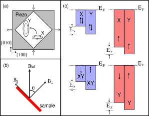
Figure 1: (color online). (a) Schematic showing the strain-induced transfer of electrons from one valley to another. (b) Orientation of the sample with respect to applied magnetic field. (c) (top) Strain-induced valley splitting in two- and single-spin systems. (bottom) Spin splitting caused by a magnetic field in two- and single-valley systems.

A perennial quest in the study of two dimensional electron systems (2DESs) has been to understand the role of electron-electron interaction. Experimental okamotoPRL99 ; shashkinPRL01 ; pudalovPRL02 ; zhuPRL03 ; tutucPRB03 ; vakiliPRL04 ; tanPRB06 and theoretical attaccalitePRL02 ; zhangPRB05 ; depaloPRL05 reports of enhanced spin susceptibility ($\chi_{s}$) in dilute systems have indeed provided solid evidence for the increasing influence of interaction at lower densities where the ratio of Coulomb to kinetic (Fermi) energy increases.footnote1 The successful growth and characterization of AlAs 2DESs depoortereAPL02 with controllable valley occupation shayeganPhysicaB06 opened up new opportunities to study the effects of interaction in the presence of two discrete degrees of freedom: spin and valley. The observation of a reduced $\chi_{s}$ in a two-valley system compared to a single-valley case, shkolnikovPRL04 was contrary to the then popular notion that a two-valley system is effectively more dilute than its single-valley counterpart due to its smaller Fermi energy. This observation has been since explained theoretically to be the result of a dominance of correlation effects.zhangPRB05 Recently, valley susceptibility ($\chi_{v}$) measurements, where the response of the system to an externally applied strain is studied, were reported mainly for the case where both spins were present.gunawanPRL06 ; footnote2 Here, we take this problem one step further by measuring $\chi_{v}$ for the case when the system is completely spin-polarized; we observe higher $\chi_{v}$ values compared to the partially-polarized case. In other words, analogous to the enhancement of $\chi_{s}$ upon complete valley-polarization, we observe an enhancement of $\chi_{v}$ upon complete spin-polarization. Our data suggest that the enhancement ensues rather abruptly when the system moves from the partial to complete spin-polarization regime.

We performed measurements on a 2DES confined to an 11 nm - thick AlAs quantum well, grown using molecular beam epitaxy on a semi-insulating GaAs (001) substrate. The AlAs well is flanked by AlGaAs barriers and is modulation-doped with Si. depoortereAPL02 We fabricated the sample using standard photolithography techniques. Contacts were made by depositing GeAuNi contacts and alloying in a reducing environment. Metallic gates were deposited on front and back of the sample, allowing us to control the 2D electron density (n). We made measurements in a ³He system with a base temperature of 0.3 K using standard low-frequency lock-in techniques.

Bulk AlAs has three ellipsoidal conduction band minima (valleys) at the X-points of the Brillouin zone. In wide AlAs quantum wells, the biaxial compressive strain due to the slightly larger lattice constant of AlAs compared to GaAs favors the occupation of the two valleys with their major axes lying in the 2D plane. shayeganPhysicaB06 We denote these valleys as X and Y, according to the direction of their major axes [see Fig. 1(a)]. They have anisotropic in-plane Fermi contours characterized by transverse and longitudinal band effective masses, m_t = 0.205m_e and m_l = 1.05m_e, where m_e is the free electron mass. This means that the relevant (density-of-states) band effective mass in our 2DES is $m_{b}$ = $\sqrt{\textit{m${}_{t}$}\textit{m${}_{l}$}}$ = 0.46m_e.

Figure 2: (color online) (a) Coincidence method of measuring $\chi_{v}^{*}$ in the partially spin-polarized regime shown for $n$ = $3.7\times 10^{11}$ cm^-2 at $\theta=0^{\circ}$. Corresponding energy diagram is shown in the top panel. The bottom panel shows the piezoresistance trace for $\nu=10$ where the maxima correspond to coincidences in the energy diagram. The inset shows energy levels for the $i=1$ peak which is also marked by the open brown circle in the top panel. (b) Similar measurements for the fully spin-polarized case taken at a high angle of $\theta=74^{\circ}$. (c) Index plot of data shown in the left and middle panels, combined with similar measurements at other $\nu$’s. The blue (open) and red (closed) symbols represent partial and complete spin-polarizations. The slopes give $\chi_{v}^{*}$.

Figure 1 shows how we achieve independent control over the valley and spin degrees of freedom via the application of in-plane uniaxial strain and external magnetic field respectively. The degeneracy between the two in-plane valleys can be broken with controllable strain, $\epsilon=\epsilon_{[100]}-\epsilon_{[010]}$ where $\epsilon_{[100]}$ and $\epsilon_{[010]}$ denote strain along the [100] and [010] crystal directions respectively. shayeganPhysicaB06 To implement this, we glue the sample on a piezo-electric actuator (piezo). shayeganPhysicaB06 A voltage bias applied to the piezo induces in-plane strain in the sample and causes a transfer of electrons from one valley to the other as depicted in Fig. 1(a). The induced valley splitting is given by $E_{v}=\epsilon E_{2}$ where $E_{2}$ is the deformation potential which has a band value of 5.8eV for AlAs. Analogous to its widely probed spin counterpart, valley susceptibility is defined gunawanPRL06 as $\chi_{v}=d\Delta n_{v}/d\epsilon$ where $\Delta n_{v}$ is the difference in the electron population in $X$ and $Y$ valleys, ($n_{Y}-n_{X}$). In a non-interacting picture, we have, $\chi_{v,b}\propto E_{2}m_{b}$. In a Fermi liquid picture, the presence of interaction is accounted for by renormalized quantities, denoted with asterisks throughout this paper. That is, in an interacting system, we have $\chi_{v}^{*}\propto E_{2}^{*}m^{*}$.

In our study we probe the system under partial and complete spin-polarizations. This is shown in Fig. 1(c) where the top schematics show how a finite valley splitting is introduced in the system when one (right) or two (left) spin species are occupied. In Fig. 1(b) we show the experimental setup which is used to control the level of spin-polarization. The sample is oriented at an angle ($\theta$) with respect to an external magnetic field so that it is subjected to both perpendicular ($B_{\perp}$) and parallel ($B_{\parallel}$) components of the field. Magnetic field introduces a Zeeman energy $E_{Z}=g\mu_{B}B_{tot}$ where $g$ is the Lande $g-$factor and $\mu_{B}$ is the Bohr magneton. At high enough $\theta$, $E_{Z}$ becomes greater than the Fermi energy ($E_{F}$) and the system becomes completely spin-polarized.

Given that spin and valley are two discrete degrees of freedom, we find it instructive to compare the measurements of $\chi_{v}^{*}$ and $\chi_{s}^{*}$ in the same system. The bottom schematics in Fig. 1(c) show the spin splitting when the sample is subjected to a magnetic field under single- (right) and two- (left) valley occupation. We will return to our $\chi_{s}^{*}$ measurements later in the paper.

In Fig. 2, we show the details of our valley susceptibility measurementsfootnote3 for $n=3.7\times 10^{11}$cm^-2. For the data of Fig. 2(a), the sample is held at a constant angle, $\theta=0^{\circ}$. The application of a magnetic field causes the formation of Landau levels (LLs) which are split by cyclotron energy, $E_{c}=\hbar eB_{\perp}/m^{*}$. The LLs of opposite spin are further split by $E_{Z}$. The corresponding energy level diagram is shown in the upper panel of Fig. 2(a). Note that, in our system, for the density shown, $E_{Z}>E_{c}$ even for $\theta=0^{\circ}$. The LLs of one spin are shown as solid lines, while the dotted lines denote LLs belonging to the opposite spin. Notice that when $\Delta\epsilon=0$ (see Ref. 17) each of these spin-split levels is doubly valley-degenerate. We then apply an in-plane strain which breaks this degeneracy and introduces a finite valley splitting. For any given $\nu$, there are specific values of $\Delta\epsilon$ at which the energy levels corresponding to the $X$ and $Y$ valleys come into coincidence. gunawanPRL06 For example, as indicated by the blue shaded region in the upper panel of Fig. 2(a), the energy gap at LL filling factor $\nu$ = 10 oscillates as the applied strain causes coincidences between the LLs, and finally saturates after the system becomes completely valley-polarized. The lower panel of Fig. 2(a) shows the corresponding piezoresistance trace. Note that a large value of gap corresponds to a minimum in the trace while a coincidence is marked by a peak. The small blue diamonds in the top panel are unresolvable in our experiment. The oscillations are periodic footnote4 and the positions of the peaks give a measure of $\chi_{v}^{*}$. gunawanPRL06 For example, the condition for coincidence at $\nu$ = 10 is $E_{v}=iE_{c}$ where $i$ is an odd integer. This condition can also be written as $E_{2}^{*}m^{*}=i\hbar eB_{\perp}/\Delta\epsilon$ or $i/\nu=(E_{2}^{*}m^{*})\times(2\pi/nh^{2})\times(\Delta\epsilon)$. In Fig. 2(c) we plot $i/\nu$ vs. $\Delta\epsilon$ (denoted by blue open points) for the data of Fig. 2(a). The periodicity of the oscillations in Fig. 2(a) implies that the resulting $i/\nu$ vs. $\Delta\epsilon$ plot is a straight line. Repeating the same measurement for different $\nu$’s, we observe that all points fall on the same blue (dashed) line, gunawanPRL06 the slope of which gives a $\nu$-independent $\chi_{v}^{*}$.

Results of similar experiments done on a completely spin-polarized system are shown in Fig. 2(b). The sample is tilted to a high tilt angle ($\theta=74^{\circ}$) so that $E_{Z}$ is larger than $E_{F}$. The corresponding fan diagram is shown in the top panel. Note how only one spin level is present. The variation of the energy gap with strain is shown for $\nu=6$ as the red shaded region. The oscillations observed in the piezoresistance shown in the bottom panel are well-described by the simple fan diagram. The plot of $i/\nu$ vs. $\Delta\epsilon$ is shown by closed red symbols in Fig. 2(c) which also includes data from similar measurements made at $\nu$ = 4 and 5. The data points all fall on the same line and give a value of $\chi_{v}^{*}$ which is higher than the partially spin-polarized case.

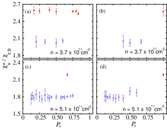
Figure 3: (color online) $\chi_{v}^{*}$, normalized to its band value, as a function of $P_{v}$ and $P_{s}$ for two densities. The blue (open) and red (closed) symbols correspond to partially and completely spin-polarized regimes respectively. Panels (a) and (b) are for $n=3.7\times 10^{11}$cm^-2 while (c) and (d) correspond to $n=5.1\times 10^{11}$cm^-2. Each data point is an average of values obtained for positive and negative values of $\Delta\epsilon$, and for different tilt angles and fillings.

Figure 2(c) suggests that $\chi_{v}^{*}$ values divide themselves into two groups corresponding to partial and complete spin-polarizations. In each of the individual branches, $\chi_{v}^{*}$ seems to be independent of the degree of valley and spin polarizations. Valley-polarization of the system at any particular $\nu$ is quantified as $P_{v}=|(n_{Y}-n_{X})/(n_{Y}+n_{X})|$ where $n_{X}$ and $n_{Y}$ denote the occupation of the $X$ and $Y$ valleys. Similarly, spin-polarization is defined as $P_{s}=|(n_{\uparrow}-n_{\downarrow})/(n_{\uparrow}+n_{\downarrow})|$ where $n_{\uparrow}$ and $n_{\downarrow}$ denote the density of electrons of up and down spins. Notice that, in general, each coincidence in the bottom panels of Figs. 2(a) and (b) corresponds to a different value of $P_{v}$ and $P_{s}$. As an example, in Fig. 2(a) we show the energy levels for the $i=1$ coincidence of $\nu=10$ as inset. In this case $P_{v}=0.2$ and $P_{s}=0.4$. In a similar way, each of the maxima in the bottom panel of Fig. 2(b) corresponds to a different value of $P_{v}$, e.g., the $i=$ 1, 3, 5 maxima correspond to $P_{v}=$ 16$\%$, 50$\%$ and 83$\%$, respectively.

To bring out the dependencies of valley susceptibility, it is instructive to plot it as an explicit function of $P_{v}$ and $P_{s}$. Note that each data point in Fig. 2(c), in general, corresponds to a different value of $P_{v}$ and $P_{s}$. From each of these points we draw a line to the origin and use the slope to determine the corresponding $\chi_{v}^{*}$. In Fig. 3(a), these $\chi_{v}^{*}$ values, averaged over positive and negative $\Delta\epsilon$, are shown as a function of $P_{v}$. The blue (open) and red (closed) symbols in Fig. 3(a) represent the partially and completely spin-polarized regimes, respectively.footnote5 The division of points into two branches corresponding to the two spin-polarization regimes is clear. Within each of these branches, we do not observe dependence on $P_{v}$. The effect of complete spin-polarization becomes more apparent in Fig. 3(b) where we plot the same points as a function of $P_{s}$. $\chi_{v}^{*}$ is independent of $P_{s}$ when $0.40<P_{s}<0.67$ but increases when the system becomes completely spin-polarized.

We repeated these measurements for various densities where larger ranges of $P_{v}$ and $P_{s}$ were accessible. Data for $n=5.1\times 10^{11}$cm^-2 are shown in Figs. 3(c) and (d). In the partially spin-polarized regime, for $0.12<P_{v}<0.75$ and $0.12<P_{s}<0.6$, we observe an almost constant $\chi_{v}^{*}$ with a very weak increase at the higher end of $P_{s}$. In the completely spin-polarized regime, we measure a much higher value of $\chi_{v}^{*}$.

Summarizing all data from different densities, we conclude that $\chi_{v}^{*}$ increases rather abruptly as the system makes a transition from partial to complete spin polarization. $\chi_{v}^{*}$ is otherwise largely independent of $P_{v}$ or $P_{s}$ in either of these regimes.

Enhancement of spin-susceptibility when valley degree of freedom is frozen out has been observed before. shkolnikovPRL04 Spin susceptibility is defined as $\chi_{s}=d\Delta n_{s}/dB$ where $\Delta n_{s}$ represents the imbalance in spin population, ($n_{\uparrow}-n_{\downarrow}$). We measured $\chi_{s}^{*}$ in our sample using the widely used coincidence technique as the tilt angle $\theta$ is varied. shkolnikovPRL04 The results of these measurements are shown side by side with $\chi_{v}^{*}$, along with the relevant polarization ranges, in Fig. 4. The left panel shows our $\chi_{v}^{*}$ measurements: the blue (open) and red (closed) symbols are for the partially and completely spin-polarized systems, respectively. Special care has been taken to make sure that, for a given $n$, $P_{v}$ is held constant while $P_{s}$ is changing from partial to complete, so that the transition from the bottom to the top branch is brought about by complete spin-polarization. The right panel of Fig. 4 shows $\chi_{s}^{*}$ measurements for single- (closed red symbols) and two- (open blue symbols) valley cases. Again, for a given $n$, $P_{s}$ is held at similar values for the top and bottom branches. We can see from this figure that $\chi_{s}^{*}$ is higher for the single-valley case compared to the two-valley case, consistent with earlier studies. shkolnikovPRL04

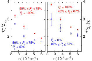
Figure 4: (color online). Summary of susceptibility data. The left panel shows $\chi_{v}^{*}$ for partial (blue circles) and complete (red squares) spin-polarization. $P_{v}$ is held constant within a narrow range to facilitate comparison. The right panel shows $\chi_{s}^{*}$ measurements for zero (blue circles) and complete (red squares) valley-polarizations. Again, $P_{s}$ is held constant within a narrow range to minimize its influence on $\chi_{s}^{*}$. Both $\chi_{v}^{*}$ and $\chi_{s}^{*}$ are normalized to their respective band values.

The most notable feature in Fig. 4 is that all susceptibilities are increasingly enhanced over their respective band values as $n$ is decreased, as expected in an interacting electron picture. Another remarkable feature is the similarity of the numerical values of $\chi_{v}^{*}$ and $\chi_{s}^{*}$ in spite of the fact that they represent the system’s response to very different external stimuli. This observation strongly suggests a parallel between spin and valley as two discreet and independent degrees of freedom. It is noteworthy though, that the values of $\chi_{v}^{*}$ and $\chi_{s}^{*}$ are not exactly the same, possibly pointing towards subtle differences.

In an earlier study, gokmenPRB07 in a wider 2DES, a weak dependence of $\chi_{s}^{*}$ on $P_{s}$ was reported in a single-valley system. For $n=5.5\times 10^{11}$cm^-2 and for $0.29\leq P_{s}\leq 0.50$, a $7\%$ variation was reported. As argued in Ref. 21, such dependence is reasonable and consistent with the large width (15nm) of the AlAs quantum well used. Since the well width of our sample is less than that used in Ref. 21, we expect a less prominent effect. Consistent with this expectation, for $n=6.0\times 10^{11}$cm^-2 and $0.15\leq P_{s}\leq 0.40$, we observe a $2.5\%$ variation of $\chi_{s}^{*}$ in a single-valley system. However, it is noteworthy that in our studies of $\chi_{v}^{*}$ in a single-spin system, we do not find evidence for dependence on $P_{v}$. This is perhaps another indication of the inequality of spin and valley degrees of freedom. The fact that the orbital wavefunction for the two spins are the same, but that this is not the case for the two valleys, could conceivably alter the effect of interaction.

In summary, we measured valley susceptibility in an AlAs 2DES as a function of both spin and valley polarizations. We observe that the value of $\chi_{v}^{*}$ undergoes a rather sudden increase as the system moves from partial to complete spin-polarization. Apart from this, $\chi_{v}^{*}$ is mostly independent of $P_{s}$ and $P_{v}$. We also measured the spin susceptibility for valley-polarized and unpolarized systems. $\chi_{s}^{*}$ is observed to be higher in a single-valley case compared to its two-valley counterpart. All susceptibilities increase as $n$ is decreased, consistent with increasing interaction.

We thank the NSF for support.

References

- (1) F.F. Fang and P.J. Stiles, Phys. Rev. 174, 823 (1968).
- (2) A.A. Shashkin, S.V. Kravchenko, V.T. Dolgopolov, and T.M. Klapwijk, Phys. Rev. Lett. 87, 086801 (2001).
- (3) V.M. Pudalov, M.E. Gershenson, H. Kojima, N. Butch, E.M. Dizhur, G. Brunthaler, A. Prinz, and G. Bauer, Phys. Rev. Lett. 88, 196404 (2002).
- (4) J. Zhu, H.L. Stormer, L.N. Pfeiffer, K.W. Baldwin, and K.W. West, Phys. Rev. Lett. 90, 056805 (2003).
- (5) E. Tutuc, S. Melinte, E.P. De Poortere, M. Shayegan, and R. Winkler, Phys. Rev. B 67, 241309(R) (2003).
- (6) K. Vakili, Y.P. Shkolnikov, E. Tutuc, E.P. De Poortere, and M. Shayegan, Phys. Rev. Lett. 92, 226401 (2004).
- (7) Y.-W. Tan, J. Zhu, H.L. Stormer, L.N. Pfeiffer, K.W. Baldwin, and K.W. West, Phys. Rev. B 73, 045334 (2006).
- (8) C. Attaccalite, S. Moroni, P. Gori-Giorgi, and G.B. Bachelet, Phys. Rev. Lett. 88, 256601 (2002).
- (9) Y. Zhang and S. Das Sarma, Phys. Rev. B 72, 075308 (2005).
- (10) S. De Palo, M. Botti, S. Moroni, and G. Senatore, Phys. Rev. Lett. 94, 226405 (2005).
- (11) The diluteness of the system is usually parameterized by the ratio of the Coulomb and Fermi energies: = = , where is the band effective mass, is the dielectric constant of the host material, and is the 2DES density. In our AlAs 2DES, = 0.46 and , where is the free space dielectric constant. A density of 3.7 1011 cm-2 corresponds to an of 16.2 for a spin and valley unpolarized system. The ratio is effectively reduced by a factor of two when the spin or valley degeneracy is lifted and by a factor of four when both degeneracies are lifted.
- (12) E.P. De Poortere, Y.P. Shkolnikov, E. Tutuc, S.J. Papadakis, M. Shayegan, E. Palm, and T. Murphy Appl. Phys. Lett. 80, 1583 (2002).
- (13) M. Shayegan, E.P. De Poortere, O. Gunawan, Y.P. Shkolnikov, E. Tutuc, and K. Vakili, Phys. Stat. Sol. (b) 243, 3629 (2006).
- (14) Y.P. Shkolnikov, K. Vakili, E.P. De Poortere, and M. Shayegan, Phys. Rev. Lett. 92, 246804 (2004).
- (15) O. Gunawan, Y.P. Shkolnikov, K. Vakili, T. Gokmen, E.P. De Poortere, and M. Shayegan, Phys. Rev. Lett. 97, 186404 (2006).
- (16) Measurements of Ref. 15 focused mainly on partially spin-polarized 2DESs. Also reported was a single data point for the fully spin-polarized case, which fell slightly above the partially-polarized data points. Not enough data points were measured, however, to reach a general conclusion.
- (17) In our AlAs 2DESs, there is a shift with , of at which the valleys are equally occupied. This is because, in a 2DES with finite layer thickness, couples to the orbital motion of electrons and shifts the energies of the two valleys by an amount that depends on the orientation of the valley’s major axis relative to the direction of [T. Gokmen et al., unpublished]. In our experiments is along [100] and shifts the -valley energy down relative to the -valley energy. To account for this shift, in Fig. 2 the x-axes are , where is the strain needed to compensate this -induced valley splitting; e.g., in Fig. 2(a) and 0.21 in Fig. 2(b).
- (18) The last oscillation in this trace does not have the same period as others. However, this is not observed in other samples and hence we ignore the last oscillation in our susceptibility determinations.
- (19) In Fig. 3(a), note that the average of the values indicated by the blue (open) symbols is very close to the value of derived from the slope indicated in Fig. 2(c). This is not surprising, given the linearity of the points in Fig. 2(c).
- (20) T.Gokmen et al., unpublished.
- (21) T. Gokmen, M. Padmanabhan, E. Tutuc, M. Shayegan, S. De Palo, S. Moroni, and G. Senatore, Phys. Rev. B 76, 233301 (2007).