Size-dependent melting: Numerical calculations of the phonon spectrum

Abstract

In order to clarify the relationship between the phonon spectra of nanoparticles and their melting temperature, we studied in detail the size-dependent low energy vibration modes. A minimum model with atoms on a lattice and harmonic potentials for neighboring atoms is used to reveal a general behavior. By calculating the phonon spectra for a series of nanoparticles of two lattice types in different sizes, we found that density of low energy modes increases as the size of nanoparticles decreases, and this density increasing causes decreasing of melting temperature. Size-dependent behavior of the phonon spectra accounts for typical properties of surface-premelting and irregular melting temperature on fine scales. These results show that our minimum model captures main physics of nanoparticles. Therefore, more physical characteristics for nanoparticles of certain types can be given by phonons and microscopic potential models.

I INTRODUCTION

The physical properties of nanosized material have attracted considerable attention because of its technological importance as well as its fundamental interest for theoretical study. One important thermodynamic property is its size-dependent melting point depression, which, in fact, has been studied for decades. This unusual behavior of nanoparticles can lead to develop new features of materials with wide applications STjong:2004 ; MZhang:2000 ; MZhao:2004 .

Experimental studies show that (with a few exceptions), for free surface nanoparticles, the melting temperature decreases with decreasing size, and has irregular variations on a fine scale FBaletto:2005 ; CWang:2005 ; MTakagi:1954 . Many theoretical models have been employed to investigate this unusual property. Of these various models we can classify them into many categories, thermodynamical models RCouchman:1979 ; PPawlow:1909 ; CWronski:1967 ; HSakai:1996 ; RVanfleet:1995 , latent heat model QJiang:1999 ; QJiang:2002 , the surface-phonon instability model MWautelet:1995 ; MWautelet:1990 ; MWautelet:1991 , the liquid drop model KNanda:2002 ; KNanda:2006 , and bond energy model WQi:2003 ; WQi:2004 . Most of these models give the result that, the nanoparticle melting temperature $T_{mn}$ relative to the bulk melting temperature $T_{mb}$ decreases linearly with size in a general form such as $T_{mn}/T_{mb}=1-A/D$, where $D$ is the nanoparticle diameter and $A$ is a constant depending upon the modeling parameters. Some other models have a nonlinear form to fit better for smaller sizes ($D<10$nm) QJiang:1999 ; ASafaei:2008 .

The melting properties of two-dimensional Penrose lattices have been studied by Huang et. al, who made use of the phonon spectrum and the Lindemann melting criterion XHuang:1992 . It showed that the boundary atoms always have larger atomic mean-squared thermal vibration amplitudes, which means lower melting temperature. We will see that a similar behavior also appears in three-dimensional lattices in our calculation.

In this paper, we study the relation between nanoparticle melting temperature and nanoparticle size by means of the phonon spectrum, and we intend to reveal the melting properties of nanoparticles from a microscopic model. With a statistical melting criterion similar to the Lindemann criterion, we found that the linear depression of nanoparticle melting temperature with decreasing size and the irregular variations on a fine scale was given in our numerical calculation by a very simple model.

II MODEL

Two three-dimensional lattice types are considered in this paper. For simplicity, we only calculate near-spherical nanoparticles in this paper. To construct such nanoparticles, first, we create the simple cubic (SC) or face-centered cubic (FCC) lattices with $n$ lattice points on the edge. Then cut an inscribed sphere in the corresponding lattice type. The lattice points on and inside the sphere are what we count in the calculation (actually there are no lattice points on the sphere for even $n$ SC lattice). Assume that there is one atom at each lattice point, which is the equilibrium position of the atom, and the surface is free. So we do not have to take surface reconstruction and relaxation into account in this calculation.

We directly calculate the phonon modes in the harmonic approximation for the two lattices of different sizes (different $n$). The interatomic potentials that we use is the spring potential

$$V = \frac{1}{2}K_{1}\sum_{\langle ij\rangle}(|\bm{r}_{0}^{i}+\bm{u}^{i}-\bm{r}_{0}^{j}-\bm{u}^{j}|-|\bm{r}_{0}^{i}-\bm{r}_{0}^{j}|)^{2}$$ (1)

$$+\frac{1}{2}K_{2}\sum_{\{ij\}}(|\bm{r}_{0}^{i}+\bm{u}^{i}-\bm{r}_{0}^{j}-\bm{u}^{j}|-|\bm{r}_{0}^{i}-\bm{r}_{0}^{j}|)^{2}$$

where $\bm{r}_{0}^{i}$ is the position of the $i$th lattice point and $\bm{u}^{i}$ is the displacement of the atom from its equilibrium position $\bm{r}_{0}^{i}$; $\langle ij\rangle$ means that the sum is taken over the nearest neighbors and $\{ij\}$ means the next-nearest neighbors; $K_{1}$ and $K_{2}$ are spring constants for the nearest and next-nearest interactions respectively. This potential ensures that the structure of nanoparticle we consider is at least one of the lowest energy structures.

Within the harmonic approximation, we can deduce that the atomic mean-squared thermal vibration amplitude $\langle u_{i\alpha}^{2}\rangle$ is

$$\langle u_{i\alpha}^{2}\rangle=\sum_{k}\frac{e_{i\alpha,k}^{2}}{m_{i}\omega_{k}}(\frac{1}{e^{\omega_{k}/T}-1}+\frac{1}{2})$$ (2)

where $i=1,2,\ldots,N$ and $N$ is the number of atoms of the nanoparticle; $\alpha=x,y,z$; $m_{i}$ is the mass of the $i$th atom; $\omega_{k}$ is the $k$th eigenfrequency, and $e_{i\alpha,k}$ is the component of the eigenvector corresponding to the $k$th eigenfrequency. We set $\hbar=k_{B}=1$ here. $\langle$ $\rangle$ means grand canonical ensemble average.

In bulk materials, the Lindemann criterion FLindemann:1910 is commonly used. It states that a material melts at the temperature at which the amplitude of thermal vibration exceeds a certain critical fraction of the interatomic distance. Experiments and simulations show that its critical value is around 0.10–0.15 in units of the interatomic distance. Lawson showed that the overall accuracy of the Lindemann criterion for the materials he considered is not better than about 30%, and he gave an improved Lindemann criterion ALawson:2001 . For irregular nanoparticles, the distance-fluctuation criterion is introduced REtters:1977 ; RBerry:1988 . It is based on the fluctuation of the distance between pairs of atoms, while the Lindemann criterion is based on the fluctuation of individual atoms relative to their average position. And it has a problem that it depends on the duration of the simulation run DFrantz:1995 ; DFrantz:2001 .

It can be seen from the expression of $\langle u_{i\alpha}^{2}\rangle$ that, when the atoms all have the same mass $m_{i}\equiv m$, the total mean-squared atomic thermal vibration amplitude $\langle u^{2}\rangle_{tot}=\displaystyle\sum_{i,\alpha}\langle u_{i\alpha}^{2}\rangle$ is determined only by the eigenfrequencies except the mass $m$, because of the orthonormality of the eigenvectors $\displaystyle\sum_{i,\alpha}e_{i\alpha,k}^{2}=1$, i.e.

$$\langle u^{2}\rangle_{tot}=\frac{1}{m}\sum_{k}\frac{1}{\omega_{k}}(\frac{1}{e^{\omega_{k}/T}-1}+\frac{1}{2}).$$ (3)

In this case, we can directly use the Lindemann criterion in our model and do not need to calculate the eigenvectors at all.

But when the atoms do not have the same mass, we have to and actually we can easily calculate each $\langle u_{i\alpha}^{2}\rangle$ numerically here. Therefor it is reasonable to use a statistical criterion like the Lindemann criterion: if more than fifty percent of the $\sqrt{\langle u_{i\alpha}^{2}\rangle}$ exceed half of the interatomic distance, the melting happens. The “fifty” and “half” are not particularly selected and can be tuned. Compared to the Lindemann criterion, the effect of using these two figures together may be too large. But obviously they can be tuned to be consistent with the Lindemann criterion. And because the model we use here is so simple and we just focus on qualitative description, there should be no problem to use these two figures in the moment. We will show that, with this statistical criterion, the linear depression of nanoparticle melting temperature with decreasing size and the irregular variations on a fine scale are reproduced in our model and a crosspoint in the phonon modes and related results are discovered when we consider $\langle u_{i\alpha}^{2}\rangle$ statistically, although we only consider the case that all the atoms have the same mass.

Actually, the eigenfrequencies depend only on the mass $m_{i}$ and the spring constant $K_{1},K_{2}$ in our model. So each $\langle u_{i\alpha}^{2}\rangle$ at a given temperature is completely determined when $m_{i}$ and $K_{1},K_{2}$ have been chosen. Different lattice spacing $a$ has different melting temperature $T_{mn}$ because of its appearance as equilibrium interatomic distance in the criterion.

III RESULTS AND DISCUSSION

In the present calculation, we only consider the case of monoatomic nanoparticles. The SC type lattice has the nearest-neighbor interaction as well as the next-nearest-neighbor interactions, while FCC type only has the nearest-neighbor interaction. We set $m_{i}\equiv m=1,K_{1}=3,K_{2}=2,a=1$ for SC and $m_{i}\equiv m=1,K_{1}=9,K_{2}=0,a=\sqrt[3]{4}$ for FCC. We choose $a=1$ for SC and $a=\sqrt[3]{4}$ for FCC so that they have the same number density.

The density of phonon modes for lattices in two different finite sizes along with their thermodynamic limit are shown in Fig. 1 for SC and FCC respectively. When the size of nanoparticle becomes larger, the profile of the density of phonon modes becomes smoother.

For the two finite sizes of SC lattices, there are both three peaks at $\omega\approx$ 2.4, 3.4, and 4.6. The peak at $\omega\approx 2.4$ lowers down with increasing size, and it becomes a shoulder at a higher frequency $\omega\approx 2.8$ ultimately in the thermodynamic limit. So does the peak at $\omega\approx 4.6$, but it increases with increasing size and the shoulder in the thermodynamic limit is at a lower frequency $\omega\approx 4.4$. The peak at $\omega\approx 3.4$ for finite sizes becomes the only peak at a higher frequency $\omega\approx 3.7$ in the thermodynamic limit. This peak in the thermodynamic limit arises from the symmetry that leads to a large number of degenerate eigenfrequencies at this value. And our calculation show that when the symmetry breaks, the degeneracy is lifted and peaks beside it appear in finite sizes. The situation for FCC lattices is similar. But there are no shoulders in the thermodynamic limit and the peak at $\omega\approx 3.5$ in the smaller finite size disappear in the larger finite size while the peak at $\omega\approx 7.5$ does not change much for FCC.

The density of phonon modes for nanoparticles of those sizes, which are smaller than the smaller finite size ($n=13$ for SC and $n=9$ for FCC) appears in Fig. 1, begins to have zigzag-like profiles and to fluctuate more and more strongly when the size gets smaller and smaller.

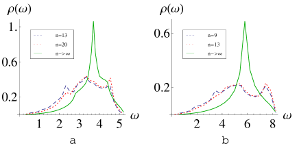
Figure 1: (Color online)Density of phonon modes for different sizes. (a) SC lattices. The dashed (blue) line is for $n=13$, the dotted (red) line is for $n=20$, and the solid (green) line is for $n\rightarrow\infty$. (b) FCC lattices. The dashed (blue) line is for $n=9$, the dotted (red) line is for $n=13$, and the solid (green) line is for $n\rightarrow\infty$. $n$ is the number of lattice points on the edge of the cubic lattice, from which we cut the inscribed sphere.

To see which phonon modes contribute to the melting, we pick out those $\langle u_{i\alpha}^{2}\rangle$ that meet our criterion and plot the mean contribution from each $[\omega,\omega+\mathrm{d}\omega]$ to $\langle u_{i\alpha}^{2}\rangle$ versus $\omega$ at the nanoparticle melting temperature determined by our model. The mean contribution from each $[\omega,\omega+\mathrm{d}\omega]$ to $\langle u_{i\alpha}^{2}\rangle$ is defined as

$$P(\omega)\equiv\frac{1}{N_{m}}{\sum_{i,\alpha}}^{\prime}\frac{\langle u_{i\alpha}^{2}\rangle_{\mathrm{d}\omega}}{\langle u_{i\alpha}^{2}\rangle}$$ (4)

where $\sum^{\prime}$ means the sum is taken over those $\langle u_{i\alpha}^{2}\rangle$ that meet our criterion, and

$$\langle u_{i\alpha}^{2}\rangle_{\mathrm{d}\omega}\equiv{\sum_{k}}^{\prime}\frac{e_{i\alpha,k}^{2}}{m_{i}\omega_{k}}(\frac{1}{e^{\omega_{k}/T}-1}+\frac{1}{2})$$ (5)

means the sum of $k$ in the expression of $\langle u_{i\alpha}^{2}\rangle$ (Eq. 2) is taken only over those $k$ that are in the range of $\omega_{k}\in[\omega,\omega+\mathrm{d}\omega]$, and $N_{m}$ means the number of those $\langle u_{i\alpha}^{2}\rangle$. We choose $\mathrm{d}\omega=0.2$ for SC and $\mathrm{d}\omega=0.4$ for FCC.

Four different finite sizes for SC and FCC lattices are shown in Fig. 2 respectively. Noted that there is a cross point in both parts of the figure, i.e. $\omega\approx 2.6$ for SC and $\omega\approx 4.5$ for FCC, so the eigenfrequencies are divided into two parts naturally: low and high eigenfrequencies. For the smallest size (the dotted lines) shown in Fig. 2, most contributions are from the low eigenfrequencies and the line fluctuates strongly in the low eigenfrequency range. With the increase of the size, the contributions from the high eigenfrequencies increase, but the increase becomes smaller and smaller; the contributions from the low eigenfrequencies get smaller with increasing size and also there is a smaller and smaller decrease, but the change is much bigger than that of the high eigenfrequencies. Apparently, a peak corresponding to the peak at $\omega\approx 2.4$ for SC and at $\omega\approx 3.5$ for FCC in Fig. 1 respectively appears in the lines (the dotdashed line and the dashed line) for the two middle sizes. Similarly, a peak corresponding to the peak at $\omega\approx 4.6$ for SC and at $\omega\approx 7.5$ for FCC appears in the line (the solid line) for the largest size in Fig. 2, which will be apparent if we plot it alone. So the line of contribution becomes more similar to the line of density of phonon modes, when the size becomes larger. The contributions almost vanish at the highest eigenfrequencies. So the low eigenfrequencies dominate the melting for relatively small nanoparticles and they can be excited at low temperature. But for relatively large nanoparticles, the high eigenfrequencies nearly give the same contributions to the melting. That is why the nanoparticle melting temperature decreases with decreasing size.

We can show that all the phonon modes with small mean neighbor relative deviations, $\langle(\bm{u}^{i}-\bm{u}^{j})^{2}\rangle$, belong to the low eigenfrequency part. We call these acoustic-like phonon modes. Most phonon modes with large mean neighbor relative deviations are within the high eigenfrequency part, and we call them optical-like phonon modes. In the acoustic-like modes, neighbor atoms tend to vibrate in the same direction similar to the acoustic modes in the diatomic linear chain; while in the optical-like modes, they prefer to vibrate in the opposite direction. So with the same thermal vibration energy, the acoustic-like modes can result in larger atomic mean-squared thermal vibration amplitude, but the optical-like modes can not do that because they have large potential energy when the neighbor atoms move to each other with small displacements.

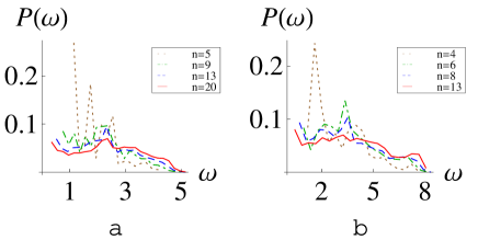
Figure 2: (Color online)Mean contributions from different eigenfrequencies to the melting. (a) SC lattices. The dotted (brown) line is for $n=5$, the dotdashed (green) line is for $n=9$, the dashed (blue) line is for $n=13$, and the solid (red) line is for $n=20$. (b) FCC lattices. The dotted (brown) line is are for $n=4$, the dotdashed (green) line is for $n=6$, the dashed (blue) line is for $n=8$, and the solid (red) line is for $n=13$. $n$ is the number of lattice points on the edge of the cubic lattice, from which we cut the inscribed sphere.

Then we divide the nanoparticle into five layers for SC and four layers for FCC, each layer having a mean radius $r$ from the center of the inscribed sphere, and plot the contributions from the low and high eigenfrequencies respectively versus $r$ (i.e. $P(r)=\frac{1}{\langle u^{2}\rangle_{tot}}\sum^{\prime\prime}\langle u_{i\alpha}^{2}\rangle_{\Delta\omega}$, where $\sum^{\prime\prime}$ means the sum is taken over those $i,\alpha$ whose corresponding atoms are in the same layer and $\langle u_{i\alpha}^{2}\rangle_{\Delta\omega}$ means the sum of $k$ in the expression of $\langle u_{i\alpha}^{2}\rangle$ is taken over those $k$ whose corresponding $\omega_{k}$ belong to the low or high eigenfrequencies; $\langle u^{2}\rangle_{tot}$ appears for normalizaion) in Fig. 4 for SC and Fig. 4 for FCC, both with four different finite sizes respectively. Here all $\langle u_{i\alpha}^{2}\rangle$ are considered no matter whether they contribute to the melting or not. This is different from Fig. 2.

Apparently, the low eigenfrequencies vibrate the atoms near the surface most, and they have nearly no effect on the inner atoms. It means surface-premelting, because the low eigenfrequencies are excited at low temperature and they mainly vibrate the atoms near the surface. This behavior should be a general property in the model similar to ours. The high eigenfrequencies vibrate the atoms in the middle when the size is relatively small, and they vibrate the atoms all but the inner ones when the size becomes large. So when most atoms are near the surface, the low eigenfrequencies is sufficient for melting because of their low excitation temperature, and when the size becomes large, more and more atoms are in the middle, the high eigenfrequencies have to be excited at high temperature for melting.

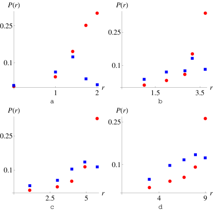
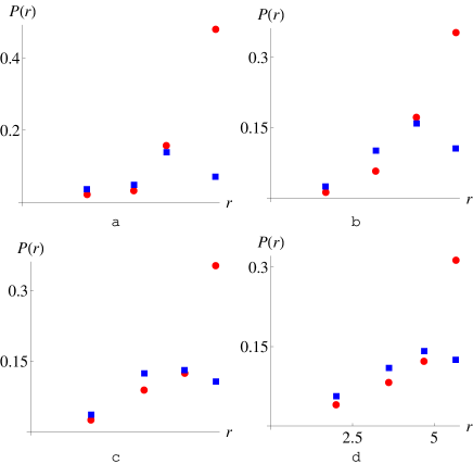
Figure 3: (Color online)Contributions from the low and high eigenfrequencies from five layers with mean radius $r$ from the center of the inscribed sphere for SC lattices. The circles (red) are for low eigenfrequencies and the squares (blue) are for high eigenfrequencies. (a) $n=5$ (b) $n=9$ (c) $n=13$ (d) $n=20$. $n$ is the number of lattice points on the edge of the cubic lattice, from which we cut the inscribed sphere.

Figure 4: (Color online)Contributions from the low and high eigenfrequencies from four layers with mean radius $r$ from the center of the inscribed sphere for FCC lattices. The circles (red) are for the low eigenfrequencies and the squares (blue) are for the high eigenfrequencies. (a) $n=4$ (b) $n=6$ (c) $n=9$ (d) $n=13$. $n$ is the number of lattice points on the edge of the cubic lattice, from which we cut the inscribed sphere.

The relation between nanoparticle melting temperature and nanoparticle size are shown in Fig. 5. The data calculated for SC and FCC lattices are fitted by $T_{mb}-A^{\prime}/D$. We do not use $1-A/D$ because we have no idea on the bulk melting temperature $T_{mb}$ for our model. It can be seen that the linear decrease of the nanoparticle melting temperature with decreasing size is reproduced for the two lattices. And the nanoparticle melting temperature fluctuates stronger with decreasing size. We think the reason is that when the size decreases, the density of phonon modes gets irregular, so it is uneasy to find a regular line to fit these small sizes. $A=A^{\prime}/T_{mb}$ is approximately 2.0 for SC and 2.5 for FCC. The difference comes from the fluctuation of the nanoparticle melting temperature of small sizes. If we only consider the large sizes calculated in our model, SC and FCC will have nearly the same $A$ in our calculation ($A=2.2$ for SC and $A=2.3$ for FCC).

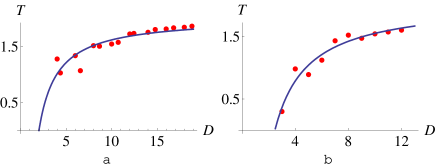
Figure 5: (Color online)The relation between nanoparticle melting temperature and nanoparticle size. (a) SC lattice. $n$ is from 5 to 20. The fit line is $T=2.03-4.06536/D$. (b) FCC lattice. $n$ is from 4 to 13. The fit line is $T=2.05495-5.07076/D$.

IV CONCLUSIONS

In this paper, we numerically calculate the phonon spectra for two types of three-dimensional lattices (SC and FCC), in the framework of a very simple microscopic model with a spring interatomic interaction within the harmonic approximation. Each spatial component of the mean-squared thermal vibration amplitude of each atom can be obtained during the calculation, and we are able to introduce a statistical melting criterion similar to the Lindemann criterion. Within this criterion, the linear decrease of the nanoparticle melting temperature with decreasing nanoparticle size and irregular variations on a fine scale are reproduced by using our simple model. And we found that the eigenfrequencies are naturally divided into two parts, the low eigenfrequency part and high eigenfrequency part, each of which ought to include all the acoustic-like and most of the optical-like modes respectively. The low eigenfrequency part played a major role in the melting of small nanoparticles, which resulted in the depression of the melting temperature. The atoms mostly near the surface are mainly vibrated in these modes, that is the so-called surface-premelting. This should be a general feature when considering the mean-squared thermal vibration amplitude of each atom independently. In this paper, we only consider the case of monoatomic nanoparticles, and the case of diatomic nanoparticles is under investigation. Moreover, we are planning to employ a more realistic interatomic interaction (including the electron-phonon coupling) and introduce relaxation of the structure in the further study.

References

- (1) S. C. Tjong and H. Chen, Mater. Sci. Eng. R. 45, 1 (2004)
- (2) M. Zhang, M. Y. U. Efremov, F. Schiettekatte, E. A. Olson, A. T. Kwan, S. L. Lai, T. Wisleder, J. E. Greene, and L. H. Allen, Phys. Rev. B 62, 10548 (2000)
- (3) M. Zhao and Q. Jiang, Solid State Commun. 130, 37 (2004)
- (4) F. Baletto and R. Ferrando, Rev. Mod. Phys. 77, 371 (2005)
- (5) C. Wang and G. Yang, Mater. Sci. Eng., R 49, 157 (2005)
- (6) M. Takagi, J. Phys. Soc. Jpn. 9, 359 (1954)
- (7) Ph. Buffat and J-P Borel, Phys. Rev. A 13, 2287 (1976).
- (8) R. R. Couchman, Philos. Mag. A 40, 637 (1979).
- (9) P. Z. Pawlow, Phys. Chem. 65, 1 (1909).
- (10) C. R. M. Wronski, Br. J. Appl. Phys. 18, 1731 (1967).
- (11) H. Sakai, Surf. Sci. 351, 285 (1996).
- (12) R. R. Vanfleet and J. M. Mochel, Surf. Sci. 341, 40 (1995).
- (13) Q. Jiang, H. Shi, and M. Zhao, J. Chem. Phys. 111, 2176 (1999).
- (14) Q. Jiang, J. Li, and B. Chi, Chem. Phys. Lett. 366, 551 (2002)
- (15) M. Wautelet, Solid State Commun. 74, 1237 (1990).
- (16) M. Wautelet, J. Phys. D 24, 343 (1991).
- (17) M. Wautelet, Eur. Phys. J. Appl. Phys. 29, 51 (2005).
- (18) K. K. Nanda, S. N. Sahu, and S. N. Behera, Phys. Rev. A 66, 013208 (2002).
- (19) K. K. Nanda, Chem. Phys. Lett. 419, 195 (2006)
- (20) W. Qi, M. Wang, and G. Xu, Chem. Phys. Lett. 372, 632 (2003)
- (21) W. Qi and M. Wang, Mater. Chem. Phys. 88, 280 (2004)
- (22) A. Safaei, M. Attarian Shandiz, S. Sanjabi, and Z. H. Barber, J. Phys. Chem. C 112, 99 (2008).
- (23) X. Huang, Y. Liu, N. Zou, and P. Ma, Phys. Rev. B 46, 10662 (1992)
- (24) F. A. Lindemann, Phys. Z. 11, 609 (1910).
- (25) A. C. Lawson, Phil. Mag. B 80, 53 (2001).
- (26) R. D. Etters and J. Kaelberer, J. Chem. Phys. 66, 5112 (1977).
- (27) R. S. Berry, T. L. Beck, H. L. Davis, and J. Jellinek, Evolution of Size Effects in Chemical Dynamics (Wiley, New York), p. 75 (1988).
- (28) D. D. Frantz, J. Chem. Phys. 102, 3747 (1995)
- (29) D. D. Frantz, J. Chem. Phys. 115, 6136 (2001)