Nonadiabatic wavepacket dynamics: -space formulation
Abstract
The time evolution of wavepackets in crystals in the presence of a homogeneous electric field is formulated in -space in a numerically tractable form. The dynamics is governed by separate equations for the motion of the waveform in -space and for the evolution of the underlying Bloch-like states. A one-dimensional tight-binding model is studied numerically, and both Bloch oscillations and Zener tunneling are observed. The long-lived Bloch oscillations of the wavepacket center under weak fields are accompanied by oscillations in its spatial spread. These are analyzed in terms of a -space expression for the spread having contributions from both the quantum metric and the Berry connection of the Bloch states. We find that when sizeable spread oscillations do occur, they are mostly due to the latter term.
pacs:
72.10.Bg, 78.20.-e, 78.20.Bh, 71.90.+qI Introduction
The study of the dynamics of electron wavepackets in crystals has experienced a revival in recent years. The development of heterostructure superlattices, photonic crystals, and optical lattices has opened new possibilities for the experimental realization of fundamental dynamical effects such as Bloch oscillationsFeldmann et al. (1992); Ben Dahan et al. (1996); Pertsch et al. (1999); Sapienza et al. (2003); Morsch et al. (2001) and Zener tunneling.Niu et al. (1996); Trompeter et al. (2006); Cristiani et al. (2002) The wavepacket picture of transport has also shed light on subtle transport phenomena in solids. For instance, the intrinsic anomalous Hall effect in ferromagnets was shown to result from a Berry-curvature term in the wavepacket group velocity.Chang and Niu (2008)
Numerical simulations provide valuable insights into the dynamics of wavepackets in crystals. For instance, Bouchard and LubanBouchard and Luban (1995) carried out a detailed study on a one-dimensional biased lattice, finding a rich variety of dynamical phenomena (Bloch oscillations of the center of mass, coherent breathing modes, Zener tunneling, and intrawell oscillations) as a function of the field-free band structure, field strength, and the form of the initial wavepacket. In order to solve numerically the time-dependent Schrödinger equation, they employed a supercell geometry with hard-wall boundary conditions; care had to be taken to ensure that the wavepacket never came close to the hard-wall boundaries for the duration of the simulation. In situations where unbounded acceleration (via Zener tunneling) of a significant portion of the wavepacket takes place, a large supercell must then be used, which may become computationally demanding. In principle that can be avoided by switching from hard-wall to periodic boundary conditions. However, the inclusion in the Hamiltonian of the nonperiodic electric field term then becomes problematic. A successful numerical strategy for describing homogeneous electric fields under periodic boundary conditions was developed in Refs. Souza et al., 2002; Umari and Pasquarello, 2002 for static fields, and generalized to time-dependent fields in Ref. Souza et al., 2004.
In Refs. Souza et al., 2002; Umari and Pasquarello, 2002; Souza et al., 2004 the goal was to solve for the electronic structure of insulators in the presence of a homogeneous field. In this work we use a similar strategy to describe wavepacket dynamics. Our starting point is to express the wavepacket as a linear superposition of Bloch states,
| (1) |
(for simplicity we shall work in one dimension), and to follow the time evolution of both the waveform and the underlying states . If a wavepacket, initially prepared in a given band, is constrained to remain in the same band at later times, one obtains the “semiclassical” approximation,which becomes exact in the adiabatic limit. Instead, we will allow for a fully unconstrained time evolution. As a result, for the states may become an admixture of several eigenstates of the crystal Hamiltonian . We shall refer to such nonadiabatic states as Bloch-like, since they retain the Bloch form, with .
The manuscript is organized as follows. The equations of motion for and , and the expressions for the center and spread of the packet in terms of them, are derived in Secs. II and III respectively. In Sec. IV we perform simulations for a one-dimensional tight-binding Hamiltonian, using a numerically tractable form, given in the Appendix, of those equations.
II Dynamical equations in -space
The wavepacket evolves according to the Schrödinger equation ()
| (2) |
where is the electric field, which can be time-dependent but must be spatially uniform. Since and enter Eq. (1) as a product, they are individually defined only up to a multiplicative factor which, because , must take the form . We fix this phase arbitrariness by choosing to be real and positive.
Inserting Eq. (1) into Eq. (2),
| (3) | |||||
where and henceforth the integration range from 0 to will be implied. Rewriting
| (4) | |||||
( and an integration by parts was performed) then yields, at each ,
| (5) | |||||
Contracting with and subtracting from the resulting equation its complex conjugate, we arrive at the equation of motion for ,
| (6) |
where the reality of was used, together with the relations and . To find the equation of motion for we plug (6) back into (5):
| (7) |
Eqs. (6)–(7) govern the coherent wavepacket dynamics. Eq. (7) was previously obtained in Ref. Souza et al., 2004, where it was shown to describe the dynamics of valence electrons in insulators under the homogeneous field . Here it describes the nonadiabatic evolution of the Bloch-like states supporting the wavepacket. As for Eq. (6), it is the familiar result for the -space dynamics of the waveform, which remains valid in the presence of interband mixing.
For numerical implementation the -derivatives must be replaced by finite-difference expressions over a -point mesh. While such discretization is straightforward for Eq. (6), Eq. (7) requires some care. As in Ref. Souza et al., 2004, we replace it with
| (8) |
where (). Unlike , lends itself to a numerically robust finite-differences representation (see Appendix).
III Wavepacket center and spread
In the previous Section we formulated the dynamics of the wavepacket (1) in terms of and . Here we shall express its center and spread in terms of those same -space quantities.
III.1 -space expressions
Let us define the generating function for the spatial distribution of the wavepacket:
| (13) |
where the second equality follows from Eq. (1) together with the identity
| (14) |
The first moment is given by
| (15) |
where is the Hermitian operator
| (16) |
and we have introduced the notation
| (17) |
The last equality in Eq. (15) follows from being real.
Next we evaluate the spread
| (18) |
For we use (15), while is given by :
| (19) |
Inserting in the last term on the RHS and then combining with Eq. (15) yields
| (20) |
where is the quantum metric,Marzari and Vanderbilt (1997)
| (21) |
All three terms in Eq. (20) are manifestly non-negative. The first one only depends on , while the remaining two also depend on the states . However, the second term is insensitive to the phases of those states (it is invariant under the gauge transformation (39)), whereas the third term is phase-dependent.
It is instructive to consider the limit of a uniform waveform, , in which becomes a Wannier function. Eq. (15) can then be recast as , where is the Berry phase associated with the manifold of states .King-Smith and Vanderbilt (1993) The first term on the RHS of Eq. (20) then vanishes identically, while the second and third terms reduce to the gauge-invariant and gauge-dependent parts of the Wannier spread for an isolated band in one dimension, given respectively by Eqs. (C12) and (C17) of Ref. Marzari and Vanderbilt, 1997.
III.2 Uncertainty relation and minimal wavepackets
An alternative decomposition of the wavepacket spread may be obtained by noting that
| (22) |
as can be readily verified using the hermiticity of and the reality of . Comparison with Eqs. (15) and (20) shows that
| (23) |
Combining this with the relation
| (24) |
yields, upon setting , , and using ,
| (25) |
In the limit of a vanishing lattice potential and (canonical momentum). Eq. (25) then reduces the familiar Heisenberg uncertainty relation.
Let us now show that (25) becomes an equality for minimal wavepackets in one dimension. Once the manifold of states and the width of the waveform are specified, all that remains is to set the phases of the and the shape of . We wish to minimize the spread (20) with respect to those two parameters. We start with the phases, which only affect the term . This term vanishes when is constant,exp in which case
| (26) |
Combining the previous two equations,
| (27) |
It can be verified that for this becomes an equality when the waveform has a Gaussian shape. In conclusion, a minimal wavepacket in one dimension is characterized by a Gaussian-shaped and a constant Berry connection in the region of -space where is non-negligible. Its spread equals
| (28) |
It was shown in Ref. Marzari and Vanderbilt, 1997 that the spread of a maximally-localized Wannier function in one dimension is . This result can be viewed as the limit of Eq. (28). In the opposite limit of a narrow waveform, the wavepacket spread becomes dominated by the term , as will be illustrated in the next Section.
IV Numerical Results
IV.1 Tight-binding model

We have applied our scheme to the same one-dimensional tight-binding model used in Ref. Souza et al., 2004. This is a three-band Hamiltonian with three atoms per unit cell of length and one orbital per atom,
| (29) |
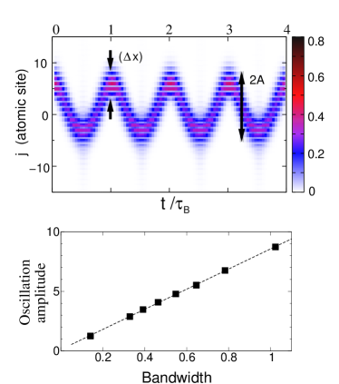
with the site energy given by . Here is the cell index, is the site index, and . The upper panel of Fig. 1 shows the energy dispersion for .
Before the spatial distribution of the wavepacket can be defined, the matrix elements of the position operator must be specified. As in Ref. Souza et al., 2004 we choose the simplest diagonal representation , with . The lower panel of Fig. 1 shows the quantum metric calculated for the Bloch states in the lowest band. As expected from the relationSouza et al. (2000) ( is the direct gap to the second band), peaks around .
We will now study numerically the wavepacket dynamics on this model. In Secs. IV.2 and IV.3 we consider respectively Bloch oscillations in a weak field and Zener tunneling in a strong field. In both cases we gradually turn on the field over a time interval, , as , and keep it constant afterwards. The simulations begin with a minimal wavepacket prepared in the lowest band. Unless otherwise noted, the width of the Gaussian waveform is .
IV.2 Bloch oscillations in a weak electric field
In order to observe long-lived Bloch oscillations we choose a weak field , which we turn on over a time interval of the order of the Bloch oscillation period (henceforth in this subsection we choose long after the field has saturated at ). 100 -points are used to sample the Brillouin zone, and the time step is .
In the upper panel of Fig. 2 the weights of the wavepacket on the tight-binding orbitals are used to depict its spatial distribution as a function of time. The Bloch oscillations of are clearly seen. In the lower panel we plot the oscillation amplitude, , versus the width, , of the lowest band, which was tuned by adjusting the tight-binding parameters in the range and . and are linearly related, with a slope . This is in agreement with the prediction , valid for a single-band tight-binding model.Bouchard and Luban (1995) The dimensionless parameter depends on the initial choice of wavepacket, but its magnitude cannot exceed ; in the present case , so that .
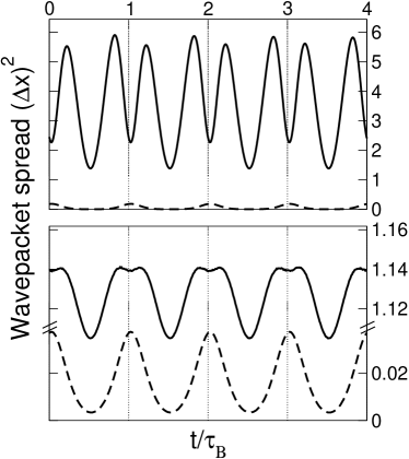
Next we analyze the behavior of the wavepacket spread in the course of the Bloch oscillations, by tracking each of the three terms in Eq. (20). According to Eq. (6), as the center of the packet traverses the Brillouin zone, the shape of the waveform remains unchanged. Hence the term is a constant of motion. Oscillations in the spread must therefore arise from the other two terms, and (henceforth the subscript will be ommited for brevity).
Since initially the wavepacket was minimal (), one might have expected spread oscillations to arise mostly from the -space dispersion of the metric, i.e., from the varying constraint imposed by the uncertainty relation (25) as the wavepacket moves through -space. Instead we find that after an initial transient the spread of the packet can become far from minimal, with (the bars denote a time average over several Bloch oscillations). This is the situation depicted in the upper panel of Fig. 3, which pertains to the same simulation run as in the upper panel of Fig. 2. Note that the spread undergoes sizeable oscillations, arising mostly from (not shown).
The above scenario is typical of Bloch oscillations in a relatively wide band. When we adjust the tight-binding parameters so as to reduce the bandwidth, we find that the wavepacket remains close to minimal in the course of the Bloch oscillations, and the associated spread oscillations are very weak, of the order of the Brillouin zone dispersion of the metric (lower panel of Fig. 3). One could try to enhance the spread oscillations by further tuning the model parameters so as to make the metric very large in some regions of -space. However, that would require very small gaps, and under those circumstances the Bloch oscillations are strongly damped by Zener tunneling.
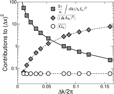
So far we have considered a fixed waveform width . Fig. 4 displays the dependence on of each contributions to , averaged over several Bloch oscillations. The term is roughly constant and equal to the Brillouin zone average of the metric; it remains a small fraction of over the entire range of . For the spread is dominated by the term , while for larger values of the term takes over. Its monotonic increase is easily understood: the larger the range , the larger the spread of over that range is likely to be.
IV.3 Zener tunneling in a strong electric field
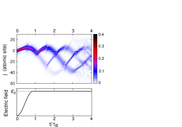
In the previous subsection a weak electric field () was chosen, so that for the duration of the simulation the wavepacket remained mostly in the lowest band. For sufficiently strong fields, significant interband transitions are expected to occur as the wavepacket reaches the zone center, where the gap is smallest. In order to observe this phenomenom the saturation field was increased from to , while the minimum gap between the first two bands was reduced from to by setting . With this choice of parameters a very good stability of the propagation algorithm is needed, and we decreased the time step from to . The Brillouin zone was sampled over 300 -points.
The Zener tunneling can be seen in the upper panel of Fig. 5 as a splitting of the wavepacket in real space, At the end of every Bloch oscillation, (, the main wavepacket in the lowest band spawns child packets which oscillate in the second band with the same period but a larger amplitude (due to the larger width of the second band) and gain more weight after each Bloch cycle. These child packets also spawn grandchild packets at , when Zener tunneling from the second to the third band becomes possible.
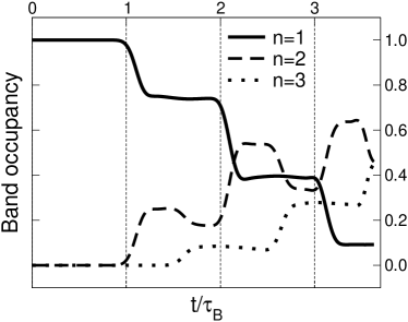
A more quantitative picture is obtained by monitoring the distribution of the packet among the three bands. We define the band occupancy as the total probability that the wavepacket resides on band :Bouchard and Luban (1995)
| (30) |
This quantity is plotted in Fig. 6 as a function of time. Initially only the first band is occupied. After a Bloch period, the wavepacket reaches the zone center, where the gap to the second band is smallest, at which point significant Zener tunneling occurs, giving rise to a partial occupation of the second band. (Between and the wavepacket moved in -space by less than the full Brillouin zone width, from to , because during most of that time interval the electric field strength was less than , as shown in the lower panel of Fig. 5.) Subsequently there are also transitions to the third band, again with periodicity ; because transitions from the second band to the first and third bands happen at the zone center and at the zone boundary respectively, undergoes changes twice as often as and .
V Conclusions
In this work we have developed a new numerical scheme for simulating wavepacket dynamics in a periodic lattice potential with a linear potential (homogeneous electric field) superimposed. By using the -space representation of the position operator, we were able to include the linear electric-field term in the Hamiltonian under periodic boundary conditions, thus avoiding having to use large supercells with hard-wall boundary conditions.Bouchard and Luban (1995)
In the present approach the wavepacket is represented on a uniform mesh of -points by a waveform sitting on top of a “band” of states [Eq. (1)]. The time evolution of the wavepacket is then obtained from that of and . For the states become non-adiabatic, field-polarized Bloch states which span several energy bands of the field-free crystal Hamiltonian (a similar representation of wavepackets in coupled energy bands was used in Ref. Culcer et al., 2005); thus interband effects such as Zener tunneling are fully accounted for.
The method was tested on a one-dimensional tight-binding model. Depending on the choice of tight-binding parameters and electric field strength, we observed either long-lived Bloch oscillations, or short-lived Bloch oscillations strongly damped by Zener tunning. In the former regime we monitored the changes in the wavepacket spread accompanying the Bloch oscillatations of the center of mass, and identified two distinct situations: (i) For wavepackets moving in narrow bands, the spread changed very little over time. (ii) For wavepackets moving in wide bands, the Bloch oscillations were accompanied by considerable oscillations of the wavepacket spread. An analysis of the -space expression for the spread [Eq. (20)] reveals two distinct contributions which can change over time: one associated with the Berry connection of the underlying Bloch states, and another related to the quantum metric. By tracking each of them separately, we concluded that in the cases where significant spread oscillations took place, they originated mostly in the Berry connection term.
Acknowledgements.
We thank David Vanderbilt for useful discussions. This work was supported by the Marie Curie OIF program of the EU and by NSF Grant No. DMR-0706493.*
Appendix A Discretized expressions in -space
Here we derive the discretized versions used in Sec. IV of the dynamical equations of Sec. II and of the wavepacket center and spread expressions of Sec. III.
A.1 Dynamical equations
The appropriate finite-difference representation of on a uniform grid isSouza et al. (2004)
| (31) |
where is the mesh spacing and
| (32) |
We use Eq. (31) to recast Eq. (8) asSouza et al. (2004)
| (33) |
in terms of the Hermitian operator
| (34) |
where and . Eq. (33) is solved numerically at each grid point usingBouchard and Luban (1995); Souza et al. (2004)
| (35) |
Because of the similarity between Eqs. (10) and (33), the phase factors can be propagated in time using the same algorithm. A finite-difference representation for the connection in Eq. (10) is needed. We useMarzari and Vanderbilt (1997)
| (36) |
where we have defined the phases . When propagating via Eq. (10), care must be taken in choosing consistently the branch cuts for the two phases in Eq. (36), to ensure that remains a smooth function of at every time step.
A.2 Wavepacket center and spread
In order to obtain a finite-difference representation of Eq. (15) we make the replacement and then use Eq. (36). A few manipulations yield
| (37) |
To find an expression for we start from Eq. (20). The first term on the RHS is easily discretized, and can be evaluated from (21). The remaining term is . For we use (37) and, from (36),
| (38) |
Besides reducing to the correct continuum expressions as , Eqs. (37) and (38) preserve exactly, for finite , certain properties of those expressions. If we perform a change of phases
| (39) |
with ( is a lattice vector and ), the center of the packet, Eq. (15), changes as
| (40) |
For a Wannier wavepacket is constant, so that the last term vanishes, and changes at most by a lattice vector.King-Smith and Vanderbilt (1993) If instead spans a narrow region of the Brillouin zone, can then shift continuously under (39). Consider the choice
| (41) |
which produces a rigid shift . Eq. (37) obeys this transformation exactly, while the spread evaluated using (38) remains unchanged, as can be easily verified.
References
- Feldmann et al. (1992) J. Feldmann, K. Leo, J. Shah, D. A. B. Miller, and J. E. Cunningham, Physical Review B 46, 7252 (1992).
- Ben Dahan et al. (1996) M. Ben Dahan, E. Peik, J. Reichel, Y. Castin, and C. Salomon, Phys. Rev. Lett. 76, 4508 (1996).
- Pertsch et al. (1999) T. Pertsch, P. Dannberg, W. Elflein, A. Bräuer, and F. Lederer, Phys. Rev. Lett. 83, 4752 (1999).
- Sapienza et al. (2003) R. Sapienza, P. Costantino, D. Wiersma, M. Ghulinyan, C. J. Oton, and L. Pavesi, Phys. Rev. Lett. 91, 263902 (2003).
- Morsch et al. (2001) O. Morsch, J. H. Müller, M. Cristiani, D. Ciampini, and E. Arimondo, Phys. Rev. Lett. 87, 140402 (2001).
- Niu et al. (1996) Q. Niu, X.-G. Zhao, G. A. Georgakis, and M. G. Raizen, Phys. Rev. Lett. 76, 4504 (1996).
- Trompeter et al. (2006) H. Trompeter, T. Pertsch, F. Lederer, D. Michaelis, U. Streppel, A. Brauer, and U. Peschel, Phys. Rev. Lett. 96, 023901 (2006).
- Cristiani et al. (2002) M. Cristiani, O. Morsch, J. H. Müller, D. Ciampini, and E. Arimondo, Phys. Rev. A 65, 063612 (2002).
- Chang and Niu (2008) M.-C. Chang and Q. Niu, J. Phys.: Condens. Matter 20, 193202 (2008).
- Bouchard and Luban (1995) A. M. Bouchard and M. Luban, Phys. Rev. B 52, 5105 (1995).
- Souza et al. (2002) I. Souza, J. Íñiguez, and D. Vanderbilt, Phys. Rev. Lett. 89, 117602 (2002).
- Umari and Pasquarello (2002) P. Umari and A. Pasquarello, Phys. Rev. Lett. 89, 157602 (2002).
- Souza et al. (2004) I. Souza, J. Íñiguez, and D. Vanderbilt, Phys. Rev. B 69, 085106 (2004).
- Marzari and Vanderbilt (1997) N. Marzari and D. Vanderbilt, Physical Review B 56, 12847 (1997).
- King-Smith and Vanderbilt (1993) R. D. King-Smith and D. Vanderbilt, Phys. Rev. B 47, 1651 (1993).
- (16) In practice a constant can be achieved on a uniform mesh following the prescription in Sec. III.C.1 of Ref. Marzari and Vanderbilt, 1997.
- Souza et al. (2000) I. Souza, T. Wilkens, and R. M. Martin, Phys. Rev. B 62, 1666 (2000).
- Culcer et al. (2005) D. Culcer, Y. Yao, and Q. Niu, Phys. Rev. B 72, 085110 (2005).