Continued Fraction Expansions of Matrix Eigenvectors

Abstract

We examine various properties of the continued fraction expansions of matrix eigenvector slopes of matrices from the $\operatorname{SL}$(2, $\mathbb{Z}$) group. We calculate the average period length, maximum period length, average period sum, maximum period sum and the distributions of 1s 2s and 3s in the periods versus the radius of the Ball within which the matrices are located. We also prove that the periods of continued fraction expansions from the real irrational roots of $x^{2}+px+q=0$ are always palindromes.

1 Introduction

Any real number $x$ can be expressed as a continued fraction of this form:

$$x=a_{0}+\cfrac{1}{a_{1}+\cfrac{1}{a_{2}+\cfrac{\dotsb}{a_{n-1}+\cfrac{1}{a_{n}+\dotsb}}}}$$

where $a_{0}\in\mathbb{Z}$ and $a_{i}\in\mathbb{Z}^{+}$ for all $i\geq 1$. For simplicity, we write $x=[a_{0},a_{1},\dotsb,a_{n},\dotsb]$. We will be looking at quadratic irrationalities, or real roots of the equation $ax^{2}+bx+c=0$ with integer $a,b,c$ . When a root is irrational, its continued fraction expansion is infinite, and always periodic past a certain index. Any rational has a finite continued fraction expansion.

In the Continued Fractions brochure by V.I. Arnold [4] he proposes this problem: ”Let us examine matrices $\begin{bmatrix}a&b\\ c&d\end{bmatrix}$, with integral $a,b,c,d$ and the determinant equal to 1. 1. We choose from these the ones that define a hyperbolic rotation. There is a finite number of matrices whose coefficients are not too large, ie. $a^{2}+b^{2}+c^{2}+d^{2}\leq N^{2}$. For each such matrix there exists an eigenvector $y=\lambda x$, for which $\lambda$ is a quadratic irrationality and therefor the continued fraction expansion of $\lambda$ is periodic. Take this period and calculate how many ones, twos, threes, etc. there are in its period, and then average this for all matrices $\begin{bmatrix}a&b\\ c&d\end{bmatrix}$. That is to say, take the number of ones in each period and divide by the number of elements in the period for each matrix. Hypothesis: this relation will approach a Gaussian distribution as $N$ approaches infinity.” (paraphrased into English from Russian. See also [3]). M.Avdeeva and B.Bykovski solved another problem posed in this broshure regarding the Gaussian distribution of period elements of continued fractions [5].

We have written a program that generates matrices $M\in\operatorname{SL}(2,\mathbb{Z})$ , such that M = $\begin{bmatrix}k&l\\ m&n\end{bmatrix}$ is within a Ball or radius $r$ around the origin for all $r\leq 1000$. That is, it generates matrices with the coefficients $k,l,m,n$ such that $k^{2}+l^{2}+m^{2}+n^{2}\leq r^{2}$ and $kn-lm=1$ . We then calculate the continued fraction expansions of the matrix eigenvector slopes and find some statistics about their periods. Because any quadratic irrationality can be expressed as the slope of an eigenvector of such a matrix, all possible quadratic irrationalities are included in our statistics as $r$ approaches infinity.

I’d like to extend a special thank you to Oleg Karpenkov for valuable help with the revision process.

2 Methods

Our program generates all matrices $M\in\operatorname{SL}(2,\mathbb{Z})$ in a ball of radius $r$ around the origin, such that M = $\begin{bmatrix}k&l\\ m&n\end{bmatrix}$ and $k\geq 0$ for all $r\leq 1000$ using the algorithm desribed in 2.1. We find one eigenvector $\begin{bmatrix}1\\ y_{1}\end{bmatrix}$ for each matrix $M$ using $y_{1}=\frac{n-k+\sqrt{(k+n)^{2}-4(kn-lm)}}{2l}$. If $y_{1}$ is real, we find the period of its continued fraction expansion using a variation of the Euclidean Algorithm described in 2.2. If $y_{1}$ is rational, we say that its period is 0. We do not make any calculations for the second eigenvector $\begin{bmatrix}1\\ y_{2}\end{bmatrix}$ of M because by Lemma 1, $y_{2}$ has the same coefficients in its period as $y_{1}$, but in reverse order. We count each matrix with coefficient $k\geq 1$ twice, because it has the same eigenvectors as the matrix $M^{{}^{\prime}}=$ $\begin{bmatrix}-k&-l\\ -m&-n\end{bmatrix}$ which we had not accounted for.

2.1 Matrix Generating Algorithm

We generate all matrices $M\in\operatorname{SL}(2,\mathbb{Z})$ in a ball of radius $r$ around the origin such that M = $\begin{bmatrix}k&l\\ m&n\end{bmatrix}$ and $k\geq 0$. We do this by generating all $k$ between $0$ and $r$. Then for each $k$ we generate all $m$ between $-\sqrt{r^{2}-k^{2}}$ and $\sqrt{r^{2}-k^{2}}$. For each $k,m$ pair, we find a solution to the Diaphontane equation $kn-lm=1$ for $l,n$. This way we obtain one matrix M = $\begin{bmatrix}k&l\\ m&n\end{bmatrix}$ for each $k,m$ pair. To obtain the rest of the matrices, we find $M_{a}=\begin{bmatrix}k&l+ak\\ m&n+am\end{bmatrix}$ for $a=0,1,2,...$ and $a=-1,-2,-3...$ such that $k^{2}+(l+ak)^{2}+m^{2}+(n+am)^{2}\leq r^{2}$.

2.2 Computing the Continued Fractions of Quadratic Irrationalities

We wish to compute the continued fraction expansion of $x_{0}=\frac{u_{0}+v_{0}\sqrt{w_{0}}}{z_{0}}$ for $u_{0}$, $v_{0}$, $w_{0}$, $z_{0}\in\mathbb{Z}$ using the Euclidean Algorithm. Let $a_{0}$ be the integer part of $x_{0}$ and let $x_{0}^{{}^{\prime}}$ be the fractional part of $x_{0}$. Then let $x_{1}=\frac{1}{x_{o^{{}^{\prime}}}}$ and $a_{1}$ be the integer part of $x_{1}$. We continue this process finding $x_{0},x_{1},\dotsb,x_{n}$ until $x_{n}=x_{i}$ for some $i<n$. Then the continued fraction expansion of $x$ is $[a_{0},a_{1},\dotsb,a_{n}]$ and the period of the continued fraction expansion is $[a_{i},a_{i+1},\dotsb,a_{n-1}]$.

Notice that $x_{1}=\frac{u_{1}+v_{1}\sqrt{w_{0}}}{z_{1}}$ for $u_{1},v_{1},z_{1}\in\mathbb{Z}$ that are easily expressed in terms of $u_{0},v_{0},z_{0}$ and $a_{0}$. V. I. Arnold conjectured that if we begin with $x_{0}$ that is a real root of $x^{2}+px+q$ for $p,q\in\mathbb{Z}$, then the $u_{i}$ and $z_{i}$ obtained through this algorithm are always divisible by $v_{i}$. In other words, we are always able to cancel out $v_{i}$ in this special case. This conjecture held in all of our calculations. Furthermore, we found that for the general case where $x_{0}$ is a real root of $ax^{2}+bx+c$ for $a,b,c\in\mathbb{Z}$ we are also able to cancel out large numbers from the numerator and denominator by finding their greatest common divisors. We noticed that after canceling, the coefficients $u_{i},v_{i},w_{i}$, and $z_{i}$ grow very little throughout the calculation of any continued fraction expansion. We compared our algorithm with the same algorithm that does not cancel out the common divisors and found that our algorithm has a significantly lower big O running time. Without canceling the coefficients grow exponentially throughout the calculation, while with canceling they are bounded.

We also discovered a better algorithm that we have not yet implemented. The idea is to find at every $i$-th step the equation $A_{i}x^{2}+B_{i}x+C_{i}$ that has the root $x_{i}$ described above. Then if we let $a_{i}$ be the integer part of $x_{i}$, the equation for $x_{i+1}$ has coefficients $A_{i+1}=A_{i}a_{i}^{2}+B_{i}a_{i}+C_{i}$ , $B_{i+1}=B_{i}+2A_{i}a_{i}$ and $C_{i+1}=A_{i}$ . Hinchin [6] proved that the coefficients $A_{i},B_{i}$ and $C_{i}$ are bounded with the bounds $C_{i}=A_{i-1}<2|A_{0}x_{0}|+|A_{0}|+|B_{0}|$ and $B_{i}$ can be defined in terms of $A_{i}$ and $C_{i}$ by $B_{i}^{2}=B_{0}^{2}-4A_{0}C_{0}+4A_{i}C_{i}$.

3 Results

3.1 Average Period Length vs. Radius

We computed the average period length of the continued fraction expansions of the slopes of matrix eigenvectors for matrices within a ball of radius $r$ around the origin for $r\leq 1000$. We did this by summing all the period lengths for matrices within a given radius and dividing by the total number of matrices with real eigenvectors and real eigenvector slopes within that radius. We plotted the average period length versus the radius as shown in Fig. 1. We found that the average period length grows as $\lg{r}$ and can be very precisely approximated by $-6.11+1.92\lg{r}$ for $r\leq 1000$.

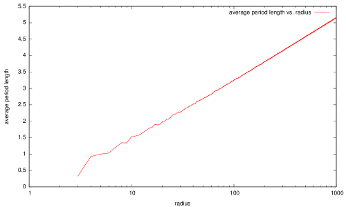
Figure 1: Average period length of continued fractions associated with matrix eigenvectors for matrices within a ball of radius r for $r\leq 1000$. It can be very precisely approximated by $-6.11+1.92\lg{r}$.

3.2 Maximum Period Length vs. Radius

We computed the maximum period length of the continued fraction expansions of the slopes of matrix eigenvectors for matrices within a ball of radius $r$ around the origin for $r\leq 1000$. We plotted the maximum period length versus the radius as shown in Fig. 2. We found that the maximum period length appears to grow as $\lg{r}$. For example, for a radius of $r=100$, the maximum period length is 8. It occurs for the matrix $M=\begin{bmatrix}8&21\\ -29&-76\end{bmatrix}$, the continued fraction expansion of whose eigenvector has the period [1, 1, 1, 1, 1, 1, 1, 2].

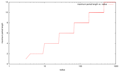
Figure 2: Maximum period length of continued fractions associated with matrix eigenvectors for matrices within a ball of radius r. The maximum period length grows as $\lg{r}$.

3.3 Average Sum of Period Elements vs. Radius

We computed the average sum of period elements of the continued fraction expansions of the slopes of matrix eigenvectors for matrices within a ball of radius $r$ around the origin for $r\leq 1000$. We did this by summing all the elements in the periods for matrices within a given radius and dividing by the total number of matrices with real eigenvectors and real eigenvector slopes within that radius. We plotted the average period sum versus the radius as shown in Fig. 3. We found that the average period sum grows faster than $\lg{r}$.

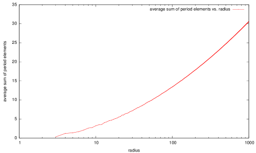
Figure 3: Average sum of period elements of continued fractions associated with matrix eigenvectors for matrices within a ball of radius r. The average period sum grows faster than $\lg{r}$.

3.4 Average of the Quantity (Period Sum / Period Length) vs. Radius

We computed the average quantity (sum of period elements / period length) of the periods of the continued fraction expansions of the slopes of matrix eigenvectors for matrices within a ball of radius $r$ around the origin for $r\leq 1000$. We did this by summing the quantities $Q_{i}$ for matrices within a given radius and dividing by the total number of matrices with real eigenvectors and real eigenvector slopes within that radius. Here $Q_{i}$ is the sum of the period elements divided by the length of the period for the $i$-th continued fraction. We plotted the average of the $Q_{i}$ versus the radius as shown in Fig. 4. We found that the average of the quantity (period sum/period length) grows as $\lg{r}$ and can be very precisely approximated by $-2.70+3.71\lg{r}$ for $r\leq 1000$.

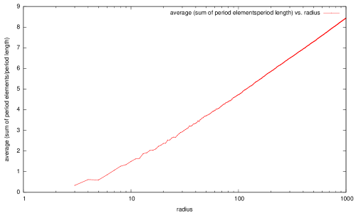
Figure 4: Average of (period sum/period length) for continued fractions associated with matrix eigenvectors for matrices within a ball of radius r. It can be very precisely approximated by $-2.70+3.71\lg{r}$ for $r\leq 1000$

3.5 Maximum Sum of Period Elements vs. Radius

We computed the maximum sum of the period elements of the continued fraction expansions of the slopes of matrix eigenvectors for matrices within a ball of radius $r$ around the origin for $r\leq 1000$. We found that for a radius $r\geq 5$ the maximum sum of the period elements is $r-2$ and occurs for the matrix $M=\begin{bmatrix}0&1\\ -1&1-r\end{bmatrix}$. The eigenvector $e_{1}=$ $\begin{bmatrix}1\\ \lambda_{1}\end{bmatrix}$ of $M$ has the slope $\lambda_{1}=$ $\frac{1-r+\sqrt{(1-r)^{2}-4}}{2}$ , which has the continued fraction expansion $[-1,1,r-3,\dotsb]$ with the period $[1,r-3]$.

3.6 Appearance of 1s 2s and 3s vs. Radius

The Gauss-Kuzmin distribution gives the probability distribution of the occurrence of a given integer in the periods of the continued fraction expansions of arbitrary real numbers. [7]. Bykovski and Avdeeva proved that this is also true for arbitrary quadratic irrationalities [5]. The percentage of 1s, 2s and 3s in the periods of the fractions that we calculated should follow the Gauss-Kuzhmin distribution

$$\Pr(K=k)=-\log_{2}\left(1-\frac{1}{(k+1)^{2}}\right).$$

So we would expect that the percentage of 1s would tend to 0.415, the percentage of 2s would tend to 0.169 and the percentage of 3s would tend to 0.093. It is evident from Fig. 5, 6 and 7 that the radius is too small for us to see this distribution.

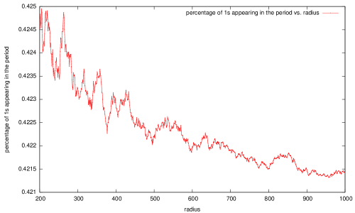
Figure 5: Percentage of 1s in the periods of continued fractions associated with matrix eigenvectors for matrices within a ball of radius r for $r\leq 1000$. The Gauss-Kuzhmin distribution requires that the percentage should tend to 0.415 as $r$ tends to infinity.

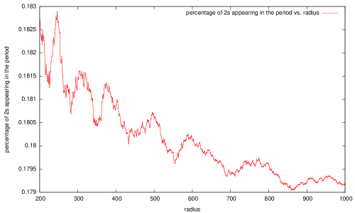
Figure 6: Percentage of 2s in the periods of continued fractions associated with matrix eigenvectors for matrices within a ball of radius r for $r\leq 1000$.The Gauss-Kuzhmin distribution requires that the percentage should tend to 0.169 as $r$ tends to infinity.

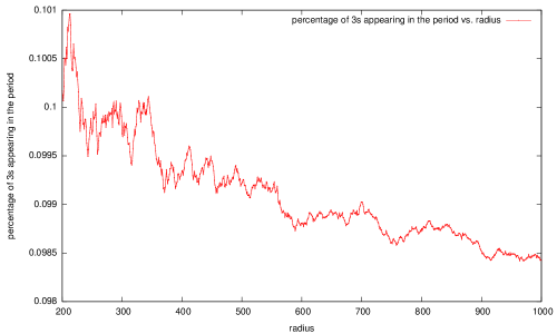
Figure 7: Percentage of 3s in the periods of continued fractions associated with matrix eigenvectors for matrices within a ball of radius r for $r\leq 1000$.The Gauss-Kuzhmin distribution requires that the percentage should tend to 0.093 as $r$ tends to infinity.

4 Palindromes Proof

Theorem 1.

Let $x_{1}$ be a real root of $x^{2}+px+q$ for $p,q\in\mathbb{Z}$. And let $[a_{0},a_{1},\dotsb,a_{n-1},a_{n}]$ be the period of the continued fraction of $x_{1}$. Then the period is a palindrome in the sense that if we look at the period as a cycle, the cycle is symmetric about some point (which might be an element of the cycle or be between two elements of the cycle). This conjecture was stated by V. I. Arnold [2] and proven by Francesca Aicardi [1]. Here is an alternate proof that we found independently.

Proof.

This proof rests on two big ideas. First, if $x_{1}$ and $x_{2}$ are real roots of

$$x^{2}+px+q$$ (1)

for $p,q\in\mathbb{Z}$, they both have the same period. This was proven by V. I. Arnold [2]. Second, Proposition 1 states that if $y_{1}$ and $y_{2}$ are real roots of any quadratic equation with integer coefficitents , they have the same coefficients in their period, but in reverse order. Because $x_{1}$ and $x_{2}$ are roots of (1), they must have the same period and the period of $x_{1}$ must be the reverse of the period of $x_{2}$. Consequently, the period of $x_{1}$ must be a palindrome. ∎

Proposition 1.

Let $y_{1}$ and $y_{2}$ be real roots of $ay^{2}+by+c$ for $a,b,c\in\mathbb{Z}$ . If we look at the period as a cycle, then the period of $y_{1}$ has the same coefficients as the period of $y_{2}$, but in reverse order.

Proof.

Lemma 1 states that if we let $M\in\operatorname{SL}(2,\mathbb{Z})$ be a matrix with eigenvectors $\begin{bmatrix}1\\ e_{1}\end{bmatrix}$ and $\begin{bmatrix}1\\ e_{2}\end{bmatrix}$, then the period of $e_{1}$, $[a_{1},a_{2},...,a_{n}]$ is the reverse of the period of $e_{2}$, $[a_{n},...a_{2},a_{1}]$. Lemma 2 states that we can construct a matrix $M\in\operatorname{SL}(2,\mathbb{Z})$ such that $\begin{bmatrix}1\\ y_{1}\end{bmatrix}$ and $\begin{bmatrix}1\\ y_{2}\end{bmatrix}$ are the eigenvectors of $M$. It follows that the period of $y_{1}$ is the reverse of the period of $y_{2}$.

∎

Lemma 1.

Let $M$ be a hyperbolic matrix in $\operatorname{SL}(2,\mathbb{Z})$ with eigenvectors $\begin{bmatrix}1\\ e_{1}\end{bmatrix}$ and $\begin{bmatrix}1\\ e_{2}\end{bmatrix}$. Then the period of $e_{1}$, $[a_{1},a_{2},...,a_{n}]$ is the reverse of the period of $e_{2}$, $[a_{n},...a_{2},a_{1}]$.

Proof.

The proof is based on the geometric interpretation of a continued fraction as the boundary of the convex hulls of integral points in the angles formed by two lines. The convex hull formed between the two eigenvectors of a matrix is invariant under a linear transformation of that matrix. The boundary is shifted by the matrix along itself. The region of the period on the boundary is shifted to another region of the period on the boundary.

Let $\lambda_{1}$ and $\lambda_{2}$ be eigenvalues of M. Because $M$ is hyperbolic and has a determinant of 1, we can assume WLOG that $|\lambda_{1}|>1$ and $|\lambda_{2}|<1$. . Therefore, by applying $M$ finitely many times, we can shift the period of $e_{1}$ onto the period of $e_{2}$. Consequently, their periods must be the reverse of one-another.

∎

Lemma 2.

Let $y_{1}$ and $y_{2}$ be real irrational roots of $ay^{2}+by+c$ for $b$, $c\in\mathbb{Z}$. Then we can construct a matrix $M\in\operatorname{SL}(2,\mathbb{Z})$ such that $\begin{bmatrix}1\\ y_{1}\end{bmatrix}$ and $\begin{bmatrix}1\\ y_{2}\end{bmatrix}$ are the eigenvectors of $M$.

Proof.

The continued fraction expansion of $y_{1}$ has some period. It is known that there exists a matrix $M\in\operatorname{SL}(2,\mathbb{Z})$ which shifts one period of $y_{1}$ into the next one and $\begin{bmatrix}1\\ y_{1}\end{bmatrix}$ is an eigenvector of $M$. We wish to shows that $\begin{bmatrix}1\\ y_{2}\end{bmatrix}$ is the other eigenvector of $M$. Let $\lambda_{1}$ and $\lambda_{2}$ be eigenvalues of $M$. Let $u=\alpha+\beta\sqrt{\gamma}$ where $\gamma$ is the discriminant of the characteristic equation of $M$ and $\alpha$ and $\beta,$ are rational. We define conjugation for $u$ as $\overline{u}$ $=\alpha-\beta\sqrt{\gamma}$. Then $y_{1}$ satisfies $[M-\lambda_{1}I]$ $\begin{bmatrix}1\\ y_{1}\end{bmatrix}$=0. Consequently it is also true that $[\overline{M}-\overline{\lambda_{1}I}]$ $\begin{bmatrix}\overline{1}\\ \overline{y_{1}}\end{bmatrix}=0$. Thus $[M-\lambda_{2}I]$ $\begin{bmatrix}1\\ y_{2}\end{bmatrix}=0$, and thus $\begin{bmatrix}1\\ y_{2}\end{bmatrix}$ is an eigenvector of $M$, as we wanted.

∎

Remark 1.

In all of our calculations the greater root of $x^{2}+px+q$ the period was always either exactly a palindrome or would be a palindrome with its first or last element removed. However, this is not always true for the periods of the lesser root. We also noticed that for $|p|,|q|\leq 100$ the period of the first root is never shifted by more than 3 places from that of the second root.

References

- [1] F. Aicardi. ? Personal Correspondence.
- [2] V. Arnold. Statistics of periods of continued fraction expansions of quadratic irrationalities (in russian).
- [3] V. Arnold. Problems Proposed by Arnold (in Russian). Fazis M., 2000.
- [4] V. Arnold. Continued Fractions (in Russian). Gosudarstevennoe Izdatel’stvo Tehniko- Teoreticheskoi Literatury, 2001.
- [5] B. Bykovski and M. Avdeeva. The solution to arnold’s problem about the gauss-kuzmin distribution (in russian). Vladivostok - Dal’nauka, 1983.
- [6] A. Hinchin. Continued Fractions (in Russian). Izdatel’stvo Moskovskovo Tsentra Heprepyvnogo Matematicheskogo Obrazovaniia, 1949.
- [7] Wikipedia. Gauss - kuzmin. http://en.wikipedia.org/wiki/Gauss-Kuzmin_distribution.