Application of two dimensional Frenkel-Kontorova model to nanotribology

Abstract

A two-dimensional Frenkel-Kontorova model is set up. Its application to the tribology is considered. The materials and the commensurability between two layers strongly affect the static friction force. It is found that the static friction force is larger between two layer of same materials than that for different materials. For two-dimensional case the averaged static friction force is larger for the uncommensurate case than that for the commensurate case, which is completely different from one-dimensional case. The directions of the propagation of the center of mass and the external driving force are usually different except at some special symmetric directions. The possibility to obtain superlubricity is suggested.

Driven dynamics of a system of interacting atoms is an interesting physical problem. It has important applications in mass and charge transport phenomena in solids and crystal surfaces. One of important applications has emerged in tribology studies, where a thin atomic layer is confined between two substrates which move respect to one another1 ; 2 . Fundamental understanding of friction is vitally important in many areas of science and technology, ranging from nanotribology to crack propagation of earthquake dynamics-1 . Progress has also been made on how to tune the intrinsic frictional forces between a sliding subject and the underlying substrate, through interface modification down to the molecular or atom scale-2 ; -3 . Such important understanding at the microscopic level, in turn, is expected to serve as important guidance in the design of smart materials with desirable lubricant properties for industrial and biomedical applications-4 ; +chen .

The application of driven Frenkel-Kontorova (FK) type model has received an increasing interest as a possible interpretative tool to understand the complex field of nanotribology9 . One dimensional FK model has been extensively studied recently13 ; +hu . However, in friction systems, an importance of higher dimensionality has been emphasized, which makes the superlubricity (the state of vanishing friction) appear much more easily–1 ; –2 ; +M.Hirano . It is found in the experimental results that by measuring the atomic-scale friction force as a function of rotational angle between two contacting layers superlubricity may appear in certain misfit angle between two layers–1 ; –2 . Friction forces completely vanish when, for example, incommensurately contacting surfaces sliding against each other. In such contact, the ratio between the lattice units of the surfaces is irrational along the sliding direction, so each individual atom receives different amounts of force from different directions. These forces consequently offset each other, resulting in zero friction. This offsetting of forces is made possible by the continuous motion of atoms, which is the basic principle behind superlubricity. Higher dimensionality of system is, therefore, crucial for atoms to move continuously. It is, therefore, necessary to extend the 1D FK model to the higher dimensions to obtain a more real model which can be realized in experiment.

For this reason, we consider an upper layer in which there are $N\times M$ atoms and they are arranged on a 2D square lattice. We first investigate the position and the velocity of an arbitrary $(n,m)$th atom, where $n=1,2,\cdots,N,m=1,2,\cdots,M$. Its position can be expressed by $\bf{r}_{n,m}=\it(x_{n,m},y_{n,m})$, where $x_{n,m}$ and $y_{n,m}$ are the positions in $x$ and $y$ directions respectively. For this arbitrary $(n,m)$th atom, the interactions among the nearest and the next nearest neighbors are considered among the upper layers. The interatomic interaction potential is chosen to be of the simple harmonic form $V_{int}=\sum_{i,j}{K\over 2}[(x_{i,j}-x_{n,m}-l)^{2}+(y_{i,j}-y_{n,m}-l)^{2}],$ with a strength $K$, a natural equilibrium spacing $l=a$ between the nearest neighbor atoms of $(n+1,m)$th, $(n-1,m)$th, $(n,m+1)$th, $(n,m-1)$th, and $l=\sqrt{2}a$ between the next nearest neighbor atoms of $(n+1,m+1)$th, $(n-1,m+1)$th, $(n+1,m-1)$th, $(n-1,m-1)$th for the upper layer.

However, this arbitrary $(n,m)$th atom not only interacts with each other among the particles in the upper layer, but also with the lower layer through a 2D periodic substrate potential which depends on the lattice structure in the lower layer. For different materials we choose different substrate potential. For generality, we choose two kinds of substrate potentials. One is with a square lattice symmetry, $V_{sqare}={f\over 2\pi}[V_{0}-\cos{2\pi x^{\prime}\over b}-\cos{2\pi y^{\prime}\over b}]$, where $f$ is the magnitude of the adhesive force between the two layers, $V_{0}$ is a constant and the length $b$ is the natural equilibrium spacing of the lower layer. The other is with a hexagonal symmetry, $V_{hexagonal}={f\over\pi}(V_{0}-\cos{2\pi x^{\prime}\over b}\cos{2\pi y^{\prime}\over\sqrt{3}b})$.

For general case of the system, in which the orientations of the two layers do not match, we rotate the two layers with respect to each other by an arbitrary misfit angle $\theta$. Then $\begin{pmatrix}x^{\prime}\\ y^{\prime}\end{pmatrix}=\begin{pmatrix}\cos{\theta}&-sin{\theta}\\ \sin{\theta}&cos{\theta}\end{pmatrix}\begin{pmatrix}x\\ y\end{pmatrix}$. The position of this arbitrary $(n,m)$th atom $\bf{r}_{n,m}$ satisfies the following equation of motion,

$$\begin{split}&\ddot{\bf{r}}_{n,m}+\gamma\dot{\bf{r}}_{n,m}+{\partial(V_{int}+V_{sub})\over\partial\bf{r}_{n,m}}=\bf{F_{\it ext}}\end{split}$$ (1)

where $\gamma$ is a phenomenology viscous damping coefficient. It can be thought of representing degrees of freedom in real physical systems which are not explicitly included in our model (e.g., vibrational or electronic excitations in the substrate). We use dimensionless variables, where identical mass $m=1$ is assigned to each atom. The frequencies of atomic vibrations are isotropic, i.e., $\omega_{x}=\omega_{y}=\sqrt{2\pi f}$, the characteristic time scale is $\tau_{0}=\sqrt{2\pi/f}$. $\bf{F_{\it ext}}=\it(F_{\it ext}\cos\alpha,F_{\it ext}\sin\alpha)$ is the external driving force, and $\alpha$ is the angle between directions of $\bf{F_{\it ext}}$ and the unit vector of $x$ axis.

A fourth-order Runge-Kutta algorithm was implemented to solve Eq.(1) numerically. The averaged velocity is defined as ${\bf{\bar{v}}}={1\over N\times M}\sum_{i=1,j=1}^{i=N,j=M}{<\textbf{\.{x}}_{i,j}>}$, where $<>$ denotes the time average. We modeled $N\times M$ atoms of upper layer and choose the periodic boundary condition to enforce a fixed density condition for the system. $x_{M+1}=x_{1}+Ma$, $y_{N+1}=y_{1}+Na$. The initial condition we choose here is that the velocity of each atom is zero and the position of each atom is at its equilibrium position. For our system we let $N=12,M=12$. In order to study how the static friction force varies with the different materials of the lower layer, the numerical simulation of the mobility as a function of the driving force and the static friction force as a function of different system parameters of both upper and lower layers are presented.

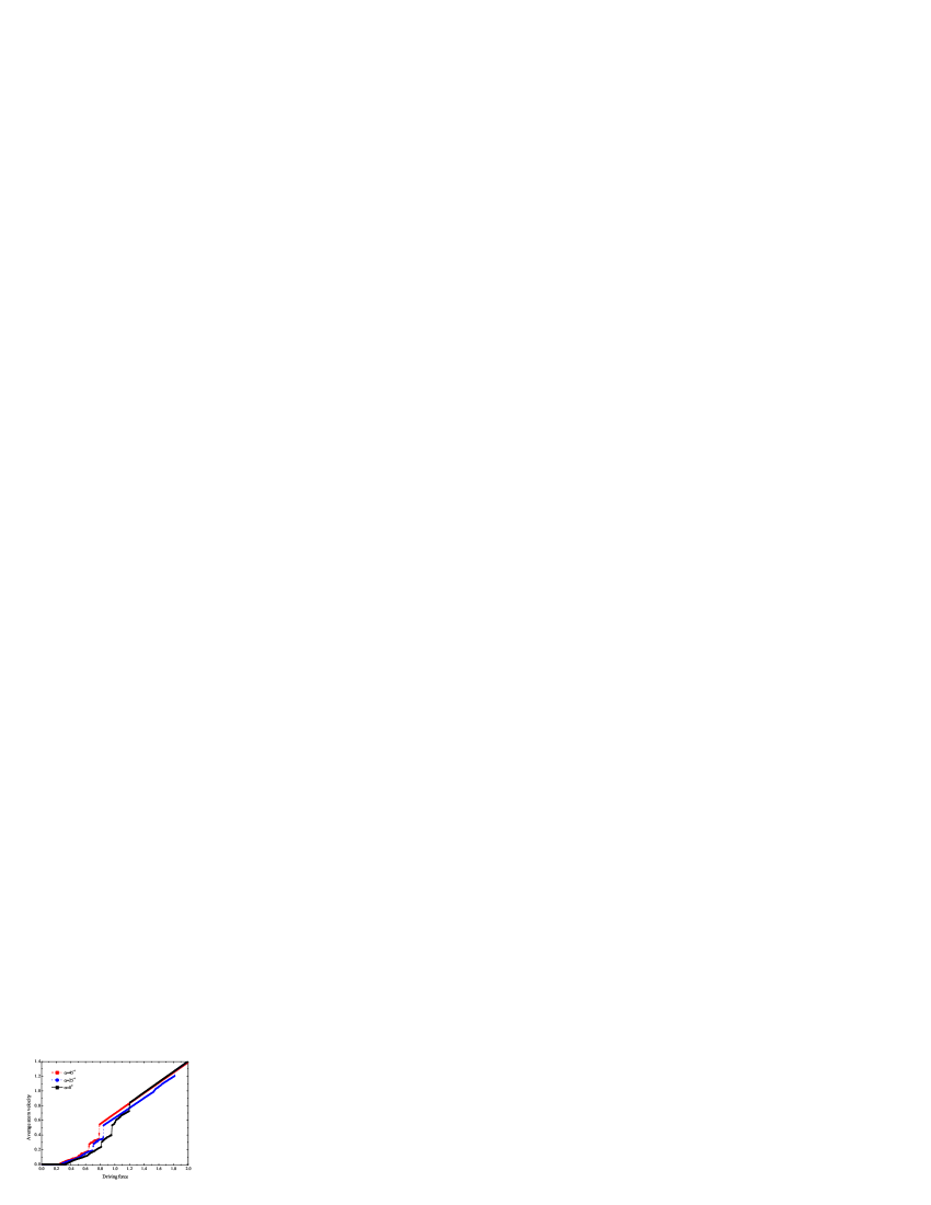
Figure 1: The mobility $<{\bf v}>$ as a function of driving force $\textbf{F}_{ext}$ for $f=1,a=b=1,m=1,K=1,\gamma=0.7$, $\theta=40^{o}$ and different values of $\alpha=0^{o},25^{o},45^{o}$.

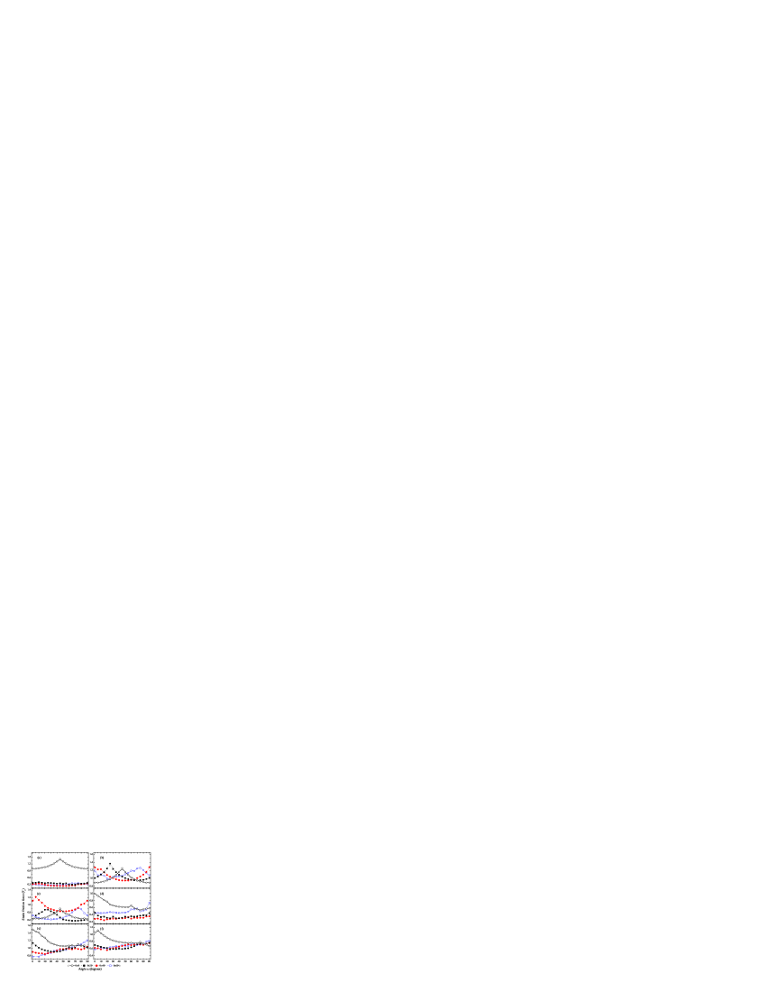
Figure 2: The numerical results of $F_{s}$ as a function of $\alpha$ in different $\theta$. (a)The commensurate case with the square symmetry substrate potential. (b)The golden mean case with the square symmetry substrate potential. (c) The spiral mean case with the square symmetry substrate potential. (d) The commensurate case with the hexagonal symmetry substrate potential. (e) The golden mean case with the hexagonal symmetry substrate potential. (f) The spiral mean case with the hexagonal symmetry substrate potential.

We define a new parameter $\beta=b/a$12 ; 10 ; 11 . For simplicity, we study three typical cases of $\beta=1$ (commensurate case), $\beta={\sqrt{5}-1\over 2}$ (golden mean case), and $\beta=0.755$ (spiral mean case), respectively, for both square and hexagonal symmetric substrate potential.

Fig.1 show the numerical results of the average chain velocity as a function of the driving force $\bf F_{\it ext}$ for the case of $\theta=40^{o}$, $K=1$, $f=1$, and $\gamma=0.7$ with different values of $\alpha$. It is for the commensurate case with square symmetric substrate potential. We note from Fig.1 that the average velocity $\bf\bar{v}$ is zero if the external force is less than $F_{s}$ (the static friction force). As the force $\bf F_{\it ext}$ increases adiabatically, the system undergoes a sharp transition from the pinned phase to the running crystal phase. Our numerical results indicate that for other values of $\theta$ the system also transfers pinning state directly to the sliding state, although $F_{s}$ is different for different $\theta$. Similar results are obtained for the case of hexagonal symmetric substrate potential. It seems that the magnitude of $F_{s}$ depends on both parameters of $\alpha$ and $\theta$. Therefore, the static friction force depends on the external driving force direction and the misfit angle. We also find from our numerical results that $F_{s}$ decreases as either $f$ decreases or $K$ increases.

In order to understand the anisotropic characters of the system the numerical results of $F_{s}$ as a function of $\alpha$ in different $\theta$ are given in Fig.2. It is noted that, for the case of square symmetric substrate potential with $\beta=1$, $F_{s}$ strongly depends on the parameter of $\theta$, especially at $\theta=0$ the static friction force $F_{s}$ is much larger than that for other values of $\theta$. $F_{s}$ also depend on the parameter of $\alpha$. But for the golden mean case and the spiral mean case the static friction forces $F_{s}$ depend on $\theta$ but not as much as that of the commensurate case of $\beta=1$ (see Figs.2(a)-2(c)). The variations of averaged friction forces with respect to $\theta$ are not as much as that of commensurate case.

Fig.2 also show how the static friction force varies with respect to different materials of the substrate. We choose two kinds of substrate materials. One is with square symmetry and the other is with hexagonal symmetry. We find that $F_{s}$ varies with different materials of the lower layer. In order to know how the static friction force depends on the different materials of the lower layer we give the averaged values of $F_{s}$ for different substrate potentials and different parameters of $\beta$ which is shown by Table 1.

Table 1 Averaged static friction forces
obtained from the numerical values of Fig.2. Upper layer Lower layer $\beta$ Averaged $F_{s}$ 1 0.521 Square lattice 0.755 0.766 Square lattice 0.618 1.058 1 0.46 Hexagonal lattice 0.755 0.713 0.618 1.013

It seems from Table 1 that the static friction force $F_{s}$ is larger between two layers of same materials than that for different materials which is in agreements with experimental resultschen2 .

Meanwhile, we note from Fig.2 that the averaged friction forces for two typical uncommensurate cases are larger than that of the commensurate case of $\beta=1$ for both square and hexagonal symmetric substrate potentials. It means that for 2D case the averaged friction force is larger for the uncommensurate case than that for the commensurate case. This result is completely different from 1D case, in which case the friction force is larger for the commensurate case than that for the uncommensurate case+M.Hirano ; 12 .

Now we analyze the atom trajectories for the case of $f=1,\gamma=0.7,a=1,b=1,K=1,\theta=40^{o},$ and $\alpha=25^{o}$ with the square symmetric substrate potential shown in Fig.1. As the external driving force increases, each atom of the system may move from its equilibrium position. Fig.3(a) present the trajectories of the $(5,4)$th, $(5,5)$th and $(5,6)$th atoms at $F_{\it ext}=0.1$. It seems that there are small displacements around their equilibrium positions for these atoms. However, the displacements are much less than lattice spacing $a$. Each atom move near its equilibrium position. However, the averaged atom velocity is still approximately zero. This state corresponds to a pinned state. When the driving force increases, the state will be transferred into a sliding state of moving crystal, see Fig.3(b) for $F_{\it ext}=1.82$, and Fig.3(c) for $F_{\it ext}=1.84$, respectively. Fig.3(b) show that the direction of average atom velocity is not same as that of the external driving force. The propagation direction of each atom is not a constant, but there are vibrations around its average direction. It actually presents a atom motion in a solitonlike fashion. We observe a formation of moving kinks for each atom. It suggest that for different driving forces the directions of average atom velocity are different. Fig.3(c) show a complete crystalline state in which case the directions between driving force and the average atom velocity are same. Although there are small vibrations between atom trajectory and the direction of the driving force, it becomes smaller and smaller as the driving force increases.

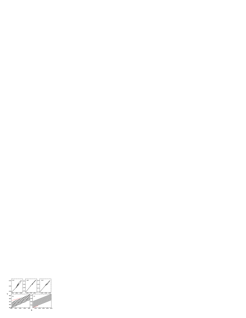
Figure 3: The trajectories of selected atoms for different external driving forces. (a) The trajectories of the atoms of $(5,4)$th, $(5,5)$th and $(5,6)$th at $F_{\it ext}=0.1$. (b) The trajectories of the atoms of $(5,1)$th, $(5,2)$th, $(5,3)$th, $(5,4)$th, $(5,5)$th, $(5,6)$th, $(5,7)$th, $(5,8)$th, $(5,9)$th, and $(5,10)$th at $F_{\it ext}=1.82$, (c) The trajectories of the atoms of $(5,1)$th, $(5,2)$th, $(5,3)$th, $(5,4)$th, $(5,5)$th, $(5,6)$th, $(5,7)$th, $(5,8)$th, $(5,9)$th, and $(5,10)$th at $F_{\it ext}=1.84$.

Fig.3 only show the trajectories of particular atoms of the system. In order to know the trajectory of mass center (c.m.) of the whole system, the differences between the direction of external driving force and the direction of trajectory of the center of mass are given in Fig.4. We define a parameter of $\alpha^{\prime}$ to represent the angle between directions of trajectory of c.m. and the unit vector of $x$ axis. The dependence of $\alpha^{\prime}$ on the external driving force are shown for $\theta=0^{o},45^{o},40^{o}$ in Fig.4(a), 4(b), 4(c), respectively. It is found that the propagation direction of the center of mass is same as that of the external driving force when $\alpha=45^{o}$ for both $\theta=0^{o}$ and $\theta=45^{o}$ due to the symmetry of the system. However, two directions are different for other cases, even for the cases of $\theta=0^{o}$ and $\theta=45^{o}$. For other values of $\theta$ two directions are different for any values of $\alpha$. We also note that if the external driving force is below the static friction force, although it is not in sliding case, the propagation direction of the center of mass is always in the direction of $\alpha^{\prime}=45^{o}$.

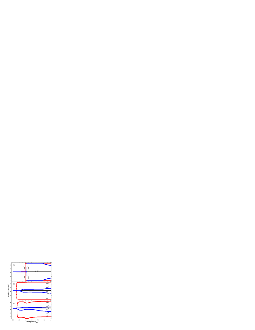
Figure 4: The angle $\alpha^{\prime}$ between the direction of trajectory of the center of mass and unit vector of $x$ axis as a function of the magnitude of the external driving force $F_{ext}$. (a)$\theta=0^{o}$. (b)$\theta=45^{o}$. (c)$\theta=40^{o}$.

In a conclusion, we find that the averaged static friction force is larger between two layers of same materials than that for different materials. For 2D case the averaged friction force is larger for uncommensurate case than that for commensurate case. To obtain superlubricity, we may choose different materials, but with commensurate ratio between two layers with larger stiffness strength $K$ of upper layer and smaller magnitude of adhesive force between two layers $f$, which may be a case of real system such as diamond-like carbon film+chen , about which superlubricity may be realized. The directions of the propagation of the center of mass and the external driving force are usually different. We may devise a experiment to verify this result in the future and it may be useful to the many fields of condensed physics, such as vortex lattices in superconductors1 ; 2 , Josephson junction, charge density waves(CDW)3 , colloids4 , Wigner crystal5 , metallic dots6 ; 7 , magnetic bubble arrays8 , etc.

The authors are grateful to the National Natural Science Foundation of P. R. China (Grant No. 50575217, 10875098 and 50421502), the Natural Science Foundation of Northwest Normal University (Grant No. NWNU-KJCXGC-03-17).

References

- (1) G. Blatter et al., Rev. Mod. Phys. 66, (1994) 1125.
- (2) M. J. Higgins and S. Bhattacharya, Phys. Rev. Lett. 74, (1995) 3029.
- (3) B. N. J. Persson, Sliding Friction, 2nd ed, (Springer, Berlin, 2000)
- (4) C. Daly and J. Krim, Phys. Rev. Lett.. 76, 803 (1996)
- (5) A. I. Volokitin and B. N. J. Persson, 91, 106101 (2003); 94, 086104 (2005)
- (6) B. N. J. Persson, O. Albolu, U. Tartaglino, A. I. Volokitin and E. Tosatti, J. Phys., Condens. Matter, 17, R1 (2005)
- (7) H. Li, T. Xu, C. Wang, J. Chen, H. Zhou, and H. Liu, Tribology International 40, (2007) 132.
- (8) B. N. J. Persson, Sliding Friction: Physical Principles and Applications sSpringer-Verlag, Berlin, 1998d; Surf. Sci. Rep.
- (9) J. Tekic, O. M. Braun, and B. Hu, Phys. Rev. E. 71 (2005) 026104.
- (10) O. M. Braun, A. R. Bishop, and J. Roder, Phys. Rev. Lett. 79, (1997) 3692; M. Paliy, O. Braun, T. Dauxois, and B. Hu, Phys. Rev. E 56, (1997) 4025; O. M. Braun, B. Hu, A. Filippov, and A. Zeltser, Phys. Rev. E 58, (1998) 1311; O. M. Braun, H. Zhang, B. Hu, and J. Tekic, Phys. Rev. E 67, (2003) 066602.
- (11) M. Hirano, K. Shinjo, R. Kaneko and Y. Murata, Phys. Rev. Lett 78, (1997) 1448.
- (12) M. Dienwiehel, G. S. Verhoeven, N. Pradeep, J. W. M. Frenken, J. A. Heimberg and H. W. Zandbergen, Phys. Rev. Lett 92, (2004) 126101.
- (13) M. Hirano, Wear. 254, (2003) 932.
- (14) A. Vanossi, N. Manini, G. Divitini, G. E. Santoro, and E. Tosatt, Phys. Rev. Lett. 97, (2006) 056101; A. Vanossi, N. Manini, F. Caruso, G. Divitini, G. E. Santoro, and E. Tosatt, Phys. Rev. Lett. 99, (2007) 206101.
- (15) A. Vanossi, A. R. Bishop, A. Franchini, and V. Bortolani, Surf. Sci. 566-568, (2004) 816-820.
- (16) A. Vanossi, J. Roder, A. R. Bishop, and V. Bortolani, Phys. Rev.E. 67, (2003) 016605.
- (17) experimental.
- (18) G. Gr ner, Rev. Mod. Phys. 60, 1129 (1988).
- (19) C. Reichhardt and C. J. Olson Reichhardt, Phys. Rev. Lett. 92, 108301 (2004).
- (20) C. Reichardt, C. J. Olson, N. Gronbech-Jensen, and F. Nori, Phys. Rev. Lett. 86, 4354 (2001).
- (21) A. A. Middleton and N. S. Wingreen, Phys. Rev. Lett. 71, 3198 (1993).
- (22) C. Reichhardt and C. J. Olson Reichhardt, Phys. Rev. Lett. 90, 046802 (2003).
- (23) R. Seshadri and R. M. Westervelt, Phys. Rev. B 46, 5150 (1992).